Chapter 6

Learning the Hidden Secrets of Data Wrangling

Learning Objectives

By the end of this chapter, you will be able to:

• Clean and handle real-life messy data
• Prepare data for data analysis by formatting data in the format required by downstream systems
• Identify and remove outliers from data

In this chapter, you will learn about data issues that happen in real-life. You will also learn how to solve these issues.

Introduction

In this chapter, we will learn about the secret sauce behind creating a successful data wrangling pipeline. In the previous chapters, we were introduced to the basic data structures and building blocks of Data Wrangling, such as pandas and NumPy. In this chapter, we will look at the data handling section of data wrangling.

Imagine that you have a database of patients who have heart diseases, and like any survey, the data is either missing, incorrect, or has outliers. Outliers are values that are abnormal and tend to be far away from the central tendency, and thus including it into your fancy machine learning model may introduce a terrible bias that we need to avoid. Often, these problems can cause a huge difference in terms of money, man-hours, and other organizational resources. It is undeniable that someone with the skills to solve these problems will prove to be an asset to an organization.

Additional Software Required for This Section

The code for this exercise depends on two additional libraries. We need to install SciPy and python-Levenshtein, and we are going to install them in the running Docker container. Be wary of this, as we are not in the container.

To install the libraries, type the following command in the running Jupyter notebook:

!pip install scipy python-Levenshtein

Advanced List Comprehension and the zip Function

In this topic, we will deep dive into the heart of list comprehension. We have already seen a basic form of it, including something as simple as a = [i for i in range(0, 30)] to something a bit more complex that involves one conditional statement. However, as we already mentioned, list comprehension is a very powerful tool and, in this topic, we will explore the power of this amazing tool further. We will investigate another close relative of list comprehension called generators, and also work with zip and its related functions and methods. By the end of this topic, you will be confident in handling complicated logical problems.

Introduction to Generator Expressions

Previously, while discussing advanced data structures, we witnessed functions such as repeat. We said that they represent a special type of function known as iterators. We also showed you how the lazy evaluation of an iterator can lead to an enormous amount of space saving and time efficiency.

Iterators are one brick in the functional programming construct that Python has to offer. Functional programming is indeed a very efficient and safe way to approach a problem. It offers various advantages over other methods, such as modularity, ease of debugging and testing, composability, formal provability (a theoretical computer science concept), and so on.

Exercise 73: Generator Expressions

In this exercise, we will be introduced to generator expressions, which are considered another brick of functional programming (as a matter of fact, they are inspired by the pure functional language known as Haskell). Since we have seen some amount of list comprehension already, generator expressions will look familiar to us. However, they also offer some advantages over list comprehension:

1. Write the following code using list comprehension to generate a list of all the odd numbers between 0 and 100,000:

   odd_numbers2 = [x for x in range(100000) if x % 2 != 0]

2. Use getsizeof from sys by using the following code:

   from sys import getsizeof

   getsizeof(odd_numbers2)

   The output is as follows:

   406496

   We will see that it takes a good amount of memory to do this. It is also not very time efficient. How can we change that? Using something like repeat is not applicable here because we need to have the logic of the list comprehension. Fortunately, we can turn any list comprehension into a generator expression.

3. Write the equivalent generator expression for the aforementioned list comprehension:

   odd_numbers = (x for x in range(100000) if x % 2 != 0)

   Notice that the only change we made is to surround the list comprehension statement with round brackets instead of square ones. That makes it shrink to only around 100 bytes! This makes it become a lazy evaluation, and thus is more efficient.

4. Print the first 10 odd numbers, as follows:

   for i, number in enumerate(odd_numbers):

   print(number)

   if i > 10:

   break

   The output is as follows:

   1

   3

   5

   7

   9

   11

   13

   15

   17

   19

   21

   23

Exercise 74: One-Liner Generator Expression

In this exercise, we will use our knowledge of generator expressions to generate an expression that will read one word at a time from a list of words and will remove newline characters at the end of them and make them lowercase. This can certainly be done using a for loop explicitly:

1. Create a words string, as follows:

   words = ["Hello ", "My name", "is ", "Bob", "How are you", "doing "]

2. Write the following generator expression to achieve the task, as follows:

   modified_words = (word.strip().lower() for word in words)

3. Create a list comprehension to get words one by one from the generator expression and finally print the list, as follows:

   final_list_of_word = [word for word in modified_words]

   final_list_of_word

   The output is as follows:

Figure 6.1: List comprehension of words

Exercise 75: Extracting a List with Single Words

If we look at the output of the previous exercise, we will notice that due to the messy nature of the source data (which is normal in the real world), we ended up with a list where, in some cases, we have more than one word together, separated by a space. To improve this, and to get a list of single words, we will have to modify the generator expressions:

1. Write the generator expression and then write the equivalent nested for loops so that we can compare the results:

   words = ["Hello ", "My name", "is ", "Bob", "How are you", "doing "]

   modified_words2 = (w.strip().lower() for word in words for w in word.split(" "))

   final_list_of_word = [word for word in modified_words2]

   final_list_of_word

   The output is as follows:

   

   Figure 6.2: List of words from the string

2. Write an equivalent to this by following a nested for loop, as follows:

   modified_words3 = []

   for word in words:

   for w in word.split(" "):

   modified_words3.append(w.strip().lower())

   modified_words3

   The output is as follows:

Figure 6.3: List of words from the string using a nested loop

We must admit that the generator expression was not only space and time saving but also a more elegant way to write the same logic.

To remember how the nested loop in generator expressions works, keep in mind that the loops are evaluated from left to right and the final loop variable (in our example, which is denoted by the single letter "w") is given back (thus we could call strip and lower on it).

The following diagram will help you remember the trick about nested for loops in list comprehension or generator expression:

Figure 6.4: Nested loops illustration

We have learned about nested for loops in generator expressions previously, but now we are going to learn about independent for loops in a generator expression. We will have two output variables from two for loops and they must be treated as a tuple so that they don't have ambiguous grammar in Python.

Create the following two lists:

marbles = ["RED", "BLUE", "GREEN"]

counts = [1, 5, 13]

You are asked to generate all possible combinations of marbles and counts after being given the preceding two lists. How will you do that? Surely using a nested for loop and with list's append method you can accomplish the task. How about a generator expression? A more elegant and easy solution is as follows:

marble_with_count = ((m, c) for m in marbles for c in counts)

This generator expression creates a tuple in each iteration of the simultaneous for loops. This code is equivalent to the following explicit code:

marble_with_count_as_list_2 = []

for m in marbles:

for c in counts:

marble_with_count_as_list_2.append((m, c))

marble_with_count_as_list_2

The output is as follows:

Figure 6.5: Appending the marbles and counts

This generator expression creates a tuple in each iteration of the simultaneous for loops. Once again, the generator expression is easy, elegant, and efficient.

Exercise 76: The zip Function

In this exercise, we will examine the zip function and compare it with the generator expression we wrote in the previous exercise. The problem with the previous generator expression is the fact that, it produced all possible combinations. For instance, if we need to relate countries with its capitals, doing so using generator expression will be difficult. Fortunately, Python gives us a built-in function called zip for just this purpose:

1. Create the following two lists:

   countries = ["India", "USA", "France", "UK"]

   capitals = ["Delhi", "Washington", "Paris", "London"]

2. Generate a list of tuples where the first element is the name of the country and the second element is the name of the capital by using the following commands:

   countries_and_capitals = [t for t in zip(countries, capitals)]

3. This is not very well represented. We can use dict where keys are the names of the countries, whereas the values are the names of the capitals by using the following command:

   countries_and_capitals_as_dict = dict(zip(countries, capitals))

   The output is as follows:

Figure 6.6: Dictionary with countries and capitals

Exercise 77: Handling Messy Data

As always, in real life, data is messy. So, the nice equal length lists of countries and capitals that we just saw are not available.

The zip function cannot be used with unequal length lists, because zip will stop working as soon as one of the lists comes to an end. To save us in such a situation, we have ziplongest in the itertools module:

1. Create two lists of unequal length, as follows:

   countries = ["India", "USA", "France", "UK", "Brasil", "Japan"]

   capitals = ["Delhi", "Washington", "Paris", "London"]

2. Create the final dict and put None as the value to the countries who do not have a capital in the capital's list:

   from itertools import zip_longest

   countries_and_capitals_as_dict_2 = dict(zip_longest(countries, capitals))

   countries_and_capitals_as_dict_2

   The output is as follows:

Figure 6.7: Output using ziplongest

We should pause here for a second and think about how many lines of explicit code and difficult-to-understand if-else conditional logic we just saved by calling a single function and just giving it the two source data lists. It is indeed amazing!

With these exercises, we are ending the first topic of this chapter. Advanced list comprehension, generator expressions, and functions such as zip and ziplongest are some very important tricks that we need to master if we want to write clean, efficient, and maintainable code. Code that does not have these three qualities are considered sub-par in the industry, and we certainly don't want to write such code.

However, we did not cover one important object here, that is, generators. Generators are a special type of function that shares the behavioral traits with generator expressions. However, being a function, they have a broader scope and they are much more flexible. We strongly encourage you to learn about them.

Data Formatting

In this topic, we will format a given dataset. The main motivations behind formatting data properly are as follows:

• It helps all the downstream systems to have a single and pre-agreed form of data for each data point, thus avoiding surprises and, in effect, breaking it.
• To produce a human-readable report from lower-level data that is, most of the time, created for machine consumption.
• To find errors in data.

There are a few ways to do data formatting in Python. We will begin with the modulus operator.

The % operator

Python gives us the % operator to apply basic formatting on data. To demonstrate this, we will load the data first by reading the CSV file, and then we will apply some basic formatting on it.

Load the data from the CSV file by using the following command:

from csv import DictReader

raw_data = []

with open("combinded_data.csv", "rt") as fd:

data_rows = DictReader(fd)

for data in data_rows:

raw_data.append(dict(data))

Now, we have a list called raw_data that contains all the rows of the CSV file. Feel free to print it to check out what it looks like.

The output is as follows:

Figure 6.8: Raw data

We will be producing a report on this data. This report will contain one section for each data point and will report the name, age, weight, height, history of family disease, and finally the present heart condition of the person. These points must be clear and easily understandable English sentences.

We do this in the following way:

for data in raw_data:

report_str = """%s is %s years old and is %s meter tall weighing about %s kg.

Has a history of family illness: %s.

Presently suffering from a heart disease: %s

""" % (data["Name"], data["Age"], data["Height"], data["Weight"], data["Disease_history"], data["Heart_problem"])

print(report_str)

The output is as follows:

Figure 6.9: Raw data in a presentable format

The % operator is used in two different ways:

• When used inside a quote, it signifies what kind of data to expect here. %s stands for string, whereas %d stands for integer. If we indicate a wrong data type, it will throw an error. Thus, we can effectively use this kind of formatting as an error filter in the incoming data.
• When we use the % operator outside the quote, it basically tells Python to start the replacement of all the data inside with the values provided for them outside.

Using the format Function

In this section, we will be looking at the exact same formatting problem, but this time we will use a more advanced approach. We will use Python's format function.

To use the format function, we do the following:

for data in raw_data:

report_str = """{} is {} years old and is {} meter tall weighing about {} kg.

Has a history of family illness: {}.

Presently suffering from a heart disease: {}

""".format(data["Name"], data["Age"], data["Height"], data["Weight"], data["Disease_history"], data["Heart_problem"])

print(report_str)

The output is as follows:

Figure 6.10: Data formatted using the format function of the string

Notice that we have replaced the %s with {} and instead of the % outside the quote, we have called the format function.

We will see how the powerful format function can make the previous code a lot more readable and understandable. Instead of simple and blank {}, we mention the key names inside and then use the special Python ** operation on a dict to unpack it and give that to the format function. It is smart enough to figure out how to replace the key names inside the quote with the values from the actual dict by using the following command:

for data in raw_data:

report_str = """{Name} is {Age} years old and is {Height} meter tall weighing about {Weight} kg.

Has a history of family illness: {Disease_history}.

Presently suffering from a heart disease: {Heart_problem}

""".format(**data)

print(report_str)

The output is as follows:

Figure 6.11: Readable file using the ** operation

This approach is indeed much more concise and maintainable.

Exercise 78: Data Representation Using {}

The {} notation inside the quote is powerful and we can change our data representation significantly by using it:

1. Change a decimal number to its binary form by using the following command:

   original_number = 42

   print("The binary representation of 42 is - {0:b}".format(original_number))

   The output is as follows:

   

   Figure 6.12: A number in its binary representation

2. Printing a string that's center oriented:

   print("{:^42}".format("I am at the center"))

   The output is as follows:

   

   Figure 6.13: A string that's been center formatted

3. Printing a string that's center oriented, but this time with padding on both sides:

   print("{:=^42}".format("I am at the center"))

   The output is as follows:

Figure 6.14: A string that's been center formatted with padding

As we've already mentioned, the format statement is a powerful one.

It is important to format date as date has various formats depending on what the source of the data is, and it may need several transformations inside the data wrangling pipeline.

We can use the familiar date formatting notations with format as follows:

from datetime import datetime

print("The present datetime is {:%Y-%m-%d %H:%M:%S}".format(datetime.utcnow()))

The output is as follows:

Figure 6.15: Data after being formatted

Compare it with the actual output of datetime.utcnow and you will see the power of this expression easily.

Identify and Clean Outliers

When confronted with real-world data, we often see a specific thing in a set of records: there are some data points that do not fit with the rest of the records. They have some values that are too big, or too small, or completely missing. These kinds of records are called outliers.

Statistically, there is a proper definition and idea about what an outlier means. And often, you need deep domain expertise to understand when to call a particular record an outlier. However, in this present exercise, we will look into some basic techniques that are commonplace to flag and filter outliers in real-world data for day-to-day work.

Exercise 79: Outliers in Numerical Data

In this exercise, we will first construct a notion of an outlier based on numerical data. Imagine a cosine curve. If you remember the math for this from high school, then a cosine curve is a very smooth curve within the limit of [1, -1]:

1. To construct a cosine curve, execute the following command:

   from math import cos, pi

   ys = [cos(i*(pi/4)) for i in range(50)]

2. Plot the data by using the following code:

   import matplotlib.pyplot as plt

   plt.plot(ys)

   The output is as follows:

   

   Figure 6.16: Cosine wave

   As we can see, it is a very smooth curve, and there is no outlier. We are going to introduce some now.

3. Introduce some outliers by using the following command:

   ys[4] = ys[4] + 5.0

   ys[20] = ys[20] + 8.0

4. Plot the curve:

   plt.plot(ys)

Figure 6.17: Wave with outliers

We can see that we have successfully introduced two values in the curve, which broke the smoothness and hence can be considered as outliers.

A good way to detect if our dataset has an outlier is to create a box plot. A boxplot is a way of plotting numerical data based on their central tendency and some buckets (in reality, we call them quartiles). In a box plot, the outliers are usually drawn as separate points. The matplotlib library helps draw boxplots out of a series of numerical data, which isn't hard at all. This is how we do it:

plt.boxplot(ys)

Once you execute the preceding code, you will be able to see that there is a nice boxplot where the two outliers that we had created are clearly shown, just like in the following diagram:

Figure 6.18: Boxplot with outliers

Z-score

A z-score is a measure on a set of data that gives you a value for each data point regarding how much that data point is spread out with respect to the standard deviation and mean of the dataset. We can use z-score to numerically detect outliers in a set of data. Normally, any data point with a z-score greater than +3 or less then -3 is considered an outlier. We can use this concept with a bit of help from the excellent SciPy and pandas libraries to filter out the outliers.

Use SciPy and calculate the z-score by using the following command:

from scipy import stats

cos_arr_z_score = stats.zscore(ys)

Cos_arr_z_score

The output is as follows:

Figure 6.19: The z-score values

Exercise 80: The Z-Score Value to Remove Outliers

In this exercise, we will discuss how to get rid of outliers in a set of data. In the last exercise, we calculated the z-score of each data point. In this exercise, we will use that to remove outliers from our data:

1. Import pandas and create a DataFrame:

   import pandas as pd

   df_original = pd.DataFrame(ys)

2. Assign outliers with a z-score less than 3:

   cos_arr_without_outliers = df_original[(cos_arr_z_score < 3)]

3. Use the print function to print the new and old shape:

   print(cos_arr_without_outliers.shape)

   print(df_original.shape)

   From the two prints (48, 1 and 50, 1), it is clear that the derived DataFrame has two rows less. These are our outliers. If we plot the cos_arr_without_outliers DataFrame, then we will see the following output:

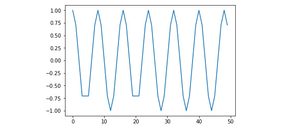
Figure 6.20: Cosine wave without outliers

As expected, we got back the smooth curve and got rid of the outliers.

Detecting and getting rid of outliers is an involving and critical process in any data wrangling pipeline. They need deep domain knowledge, expertise in descriptive statistics, mastery over the programming language (and all the useful libraries), and a lot of caution. We recommend being very careful when doing this operation on a dataset.

Exercise 81: Fuzzy Matching of Strings

In this exercise, we will look into a slightly different problem which, at the first glance, may look like an outlier. However, upon careful examination, we will see that it is indeed not, and we will learn about a useful concept that is sometimes referred to as fuzzy matching of strings.

Levenshtein distance is an advanced concept. We can think of it as the minimum number of single-character edits that are needed to convert one string into another. When two strings are identical, the distance between them is 0 – the more the difference, the higher the number. We can consider a threshold of distance under which we will consider two strings as the same. Thus, we can not only rectify human error but also spread a safety net so that we don't pass all the candidates.

Levenshtein distance calculation is an involving process, and we are not going to implement it from scratch here. Thankfully, like a lot of other things, there is a library available for us to do this. It is called python-Levenshtein:

1. Create the load data of a ship on three different dates:
   

   Figure 6.21: Initialized ship_data variable

   If you look carefully, you will notice that the name of the ship is spelled differently in all three different cases. Let's assume that the actual name of the ship is "Sea Princess". From a normal perspective, it does look like there had been a human error and the data points do describe a single ship. Removing two of them on a strict basis of outliers may not be the best thing to do.

2. Then, we simply need to import the distance function from it and pass two strings to it to calculate the distance between them:

   from Levenshtein import distance

   name_of_ship = "Sea Princess"

   for k, v in ship_data.items():

   print("{} {} {}".format(k, name_of_ship, distance(name_of_ship, k)))

   The output is as follows:

Figure 6.22: Distance between the strings

We will notice that the distance between the strings are different. It is 0 when they are identical, and it is a positive integer when they are not. We can use this concept in our data wrangling jobs and say that strings with distance less than or equal to a certain number is the same string.

Here, again, we need to be cautious about when and how to use this kind of fuzzy string matching. Sometimes, they are needed, and other times they will result in a very bad bug.

Activity 8: Handling Outliers and Missing Data

In this activity, we will identify and get rid of outliers. Here, we have a CSV file. The goal here is to clean the data by using the knowledge that we have learned about so far and come up with a nicely formatted DataFrame. Identify the type of outliers and their effect on the data and clean the messy data.

The steps that will help you solve this activity are as follows:

1. Read the visit_data.csv file.
2. Check for duplicates.
3. Check if any essential column contains NaN.
4. Get rid of the outliers.
5. Report the size difference.
6. Create a box plot to check for outliers.
7. Get rid of any outliers.

   Note

   The solution for this activity can be found on page 312.

Summary

In this chapter, we learned about interesting ways to deal with list data by using a generator expression. They are easy and elegant and once mastered, they give us a powerful trick that we can use repeatedly to simplify several common data wrangling tasks. We also examined different ways to format data. Formatting of data is not only useful for preparing beautiful reports – it is often very important to guarantee data integrity for the downstream system.

We ended the chapter by checking out some methods to identify and remove outliers. This is important for us because we want our data to be properly prepared and ready for all our fancy downstream analysis jobs. We also observed how important it is to take time and use domain expertise to set up rules for identifying outliers, as doing this incorrectly can do more harm than good.

In the next chapter, we will cover the how to read web pages, XML files, and APIs.