Chapter 4

A Deep Dive into Data Wrangling with Python

Learning Objectives

By the end of this chapter, you will be able to:

• Perform subsetting, filtering, and grouping on pandas DataFrames
• Apply Boolean filtering and indexing from a DataFrame to choose specific elements
• Perform JOIN operations in pandas that are analogous to the SQL command
• Identify missing or corrupted data and choose to drop or apply imputation techniques on missing or corrupted data

In this chapter, we will learn about pandas DataFrames in detail.

Introduction

In this chapter, we will learn about several advanced operations involving pandas DataFrames and NumPy arrays. On completing the detailed activity for this chapter, you will have handled real-life datasets and understood the process of data wrangling.

Subsetting, Filtering, and Grouping

One of the most important aspects of data wrangling is to curate the data carefully from the deluge of streaming data that pours into an organization or business entity from various sources. Lots of data is not always a good thing; rather, data needs to be useful and of high-quality to be effectively used in downstream activities of a data science pipeline such as machine learning and predictive model building. Moreover, one data source can be used for multiple purposes and this often requires different subsets of data to be processed by a data wrangling module. This is then passed on to separate analytics modules.

For example, let's say you are doing data wrangling on US State level economic output. It is a fairly common scenario that one machine learning model may require data for large and populous states (such as California, Texas, and so on), while another model demands processed data for small and sparsely populated states (such as Montana or North Dakota). As the frontline of the data science process, it is the responsibility of the data wrangling module to satisfy the requirements of both these machine learning models. Therefore, as a data wrangling engineer, you have to filter and group data accordingly (based on the population of the state) before processing them and producing separate datasets as the final output for separate machine learning models.

Also, in some cases, data sources may be biased, or the measurement may corrupt the incoming data occasionally. It is a good idea to try to filter only the error-free, good data for downstream modeling. From these examples and discussions, it is clear that filtering and grouping/bucketing data is an essential skill to have for any engineer that's engaged in the task of data wrangling. Let's proceed to learn about a few of these skills with pandas.

Exercise 48: Loading and Examining a Superstore's Sales Data from an Excel File

In this exercise, we will load and examine an Excel file.

1. To read an Excel file into pandas, you will need a small package called xlrd to be installed on your system. If you are working from inside this book's Docker container, then this package may not be available next time you start your container, and you have to follow the same step. Use the following code to install the xlrd package:

   !pip install xlrd

2. Load the Excel file from GitHub by using the simple pandas method read_excel:

   import numpy as np

   import pandas as pd

   import matplotlib.pyplot as plt

   df = pd.read_excel("Sample - Superstore.xls")

   df.head()

   Examine all the columns and check if they are useful for analysis:

   

   Figure 4.1 Output of the Excel file in a DataFrame

   On examining the file, we can see that the first column, called Row ID, is not very useful.

3. Drop this column altogether from the DataFrame by using the drop method:

   df.drop('Row ID',axis=1,inplace=True)

4. Check the number of rows and columns in the newly created dataset. We will use the shape function here:

   df.shape

   The output is as follows:

   (9994, 20)

   We can see that the dataset has 9,994 rows and 20 columns.

Subsetting the DataFrame

Subsetting involves the extraction of partial data based on specific columns and rows, as per business needs. Suppose we are interested only in the following information from this dataset: Customer ID, Customer Name, City, Postal Code, and Sales. For demonstration purposes, let's assume that we are only interested in 5 records – rows 5-9. We can subset the DataFrame to extract only this much information using a single line of Python code.

Use the loc method to index the dataset by name of the columns and index of the rows:

df_subset = df.loc[

[i for i in range(5,10)],

['Customer ID','Customer Name','City','Postal Code',

'Sales']]

df_subset

The output is as follows:

Figure 4.2: DataFrame indexed by name of the columns

We need to pass on two arguments to the loc method – one for indicating the rows, and another for indicating the columns. These should be Python lists.

For the rows, we have to pass a list [5,6,7,8,9], but instead of writing that explicitly, we use a list comprehension, that is, [i for i in range(5,10)].

Because the columns we are interested in are not contiguous, we cannot just put a continuous range and need to pass on a list containing the specific names. So, the second argument is just a simple list with specific column names.

The dataset shows the fundamental concepts of the process of subsetting a DataFrame based on business requirements.

An Example Use Case: Determining Statistics on Sales and Profit

This quick section shows a typical use case of subsetting. Suppose we want to calculate descriptive statistics (mean, median, standard deviation, and so on) of records 100-199 for sales and profit. This is how subsetting helps us to achieve that:

df_subset = df.loc[[i for i in range(100,200)],['Sales','Profit']]

df_subset.describe()

The output is as follows:

Figure 4.3 Output of descriptive statistics of data

Furthermore, we can create boxplots of sales and profit figures from this final data.

We simply extract records 100-199 and run the describe function on it because we don't want to process all the data! For this particular business question, we are only interested in sales and profit numbers and therefore we should not take the easy route and run a describe function on all the data. For a real-life dataset, the number of rows and columns could often be in the millions, and we don't want to compute anything that is not asked for in the data wrangling task. We always aim to subset the exact data that is needed to be processed and run statistical or plotting functions on that partial data:

Figure 4.4: Boxplot of sales and profit

Exercise 49: The unique Function

Before continuing further with filtering methods, let's take a quick detour and explore a super useful function called unique. As the name suggests, this function is used to scan through the data quickly and extract only the unique values in a column or row.

After loading the superstore sales data, you will notice that there are columns like "Country", "State", and "City". A natural question will be to ask how many countries/states/cities are present in the dataset:

1. Extract the countries/states/cities for which the information is in the database, with one simple line of code, as follows:

   df['State'].unique()

   The output is as follows:

   

   Figure 4.5: Different states present in the dataset

   You will see a list of all the states whose data is present in the dataset.

2. Use the nunique method to count the number of unique values, like so:

   df['State'].nunique()

   The output is as follows:

   49

   This returns 49 for this dataset. So, one out of 50 states in the US does not appear in this dataset.

Similarly, if we run this function on the Country column, we get an array with only one element, United States. Immediately, we can see that we don't need to keep the country column at all, because there is no useful information in that column except that all the entries are the same. This is how a simple function helped us to decide about dropping a column altogether – that is, removing 9,994 pieces of unnecessary data!

Conditional Selection and Boolean Filtering

Often, we don't want to process the whole dataset and would like to select only a partial dataset whose contents satisfy a particular condition. This is probably the most common use case of any data wrangling task.

In the context of our superstore sales dataset, think of these common questions that may arise from the daily activity of the business analytics team:

• What are the average sales and profit figures in California?
• Which states have the highest and lowest total sales?
• What consumer segment has the most variance in sales/profit?
• Among the top 5 states in sales, which shipping mode and product category are the most popular choices?

Countless examples can be given where the business analytics team or the executive management want to glean insight from a particular subset of data that meet certain criteria.

If you have any prior experience with SQL, you will know that these kinds of questions require fairly complex SQL query writing. Remember the WHERE clause?

We will show you how to use conditional subsetting and Boolean filtering to answer such questions.

First, we need to understand the critical concept of boolean indexing. This process essentially accepts a conditional expression as an argument and returns a dataset of booleans in which the TRUE value appears in places where the condition was satisfied. A simple example is shown in the following code. For demonstration purposes, we subset a small dataset of 10 records and 3 columns:

df_subset = df.loc[[i for i in range (10)],['Ship Mode','State','Sales']]

df_subset

The output is as follows:

Figure 4.6: Sample dataset

Now, if we just want to know the records with sales higher than $100, then we can write the following:

df_subset>100

This produces the following boolean DataFrame:

Figure 4.7: Records with sales higher than $100

Note the True and False entries in the Sales column. Values in the Ship Mode and State columns were not impacted by this code because the comparison was with a numerical quantity, and the only numeric column in the original DataFrame was Sales.

Now, let's see what happens if we pass this boolean DataFrame as an index to the original DataFrame:

df_subset[df_subset>100]

The output is as follows:

Figure 4.8: Results after passing the boolean DataFrame as an index to the original DataFrame

The NaN values came from the fact that the preceding code tried to create a DataFrame with TRUE indices (in the Boolean DataFrame) only.

The values which were TRUE in the boolen DataFrame were retained in the final output DataFrame.

The program inserted NaN values for the rows where data was not available (because they were discarded due to the Sales value being < $100).

Now, we probably don't want to work with this resulting DataFrame with NaN values. We wanted a smaller DataFrame with only the rows where Sales > $100. We can achieve that by simply passing only the Sales column:

df_subset[df_subset['Sales']>100]

This produces the expected result:

Figure 4.9: Results after removing the NaN values

We are not limited to conditional expressions involving numeric quantities only. Let's try to extract high sales values (> $100) for entries that do not involve Colorado.

We can write the following code to accomplish that:

df_subset[(df_subset['State']!='Colorado') & (df_subset['Sales']>100)]

Note the use of a conditional involving string. In this expression, we are joining two conditionals by an & operator. Both conditions must be wrapped inside parentheses.

The first conditional expression simply matches the entries in the State column to the string Colorado and assigns TRUE/FALSE accordingly. The second conditional is the same as before. Together, joined by the & operator, they extract only those rows for which State is not Colorado and Sales is > $100. We get the following result:

Figure 4.10: Results where State is not California and Sales is higher than $100

Note

Although, in theory, there is no limit on how complex a conditional you can build using individual expressions and & (LOGICAL AND) and | (LOGICAL OR) operators, it is advisable to create intermediate boolean DataFrames with limited conditional expressions and build your final DataFrame step by step. This keeps the code legible and scalable.

Exercise 50: Setting and Resetting the Index

Sometimes, we may need to reset or eliminate the default index of a DataFrame and assign a new column as an index:

1. Create the matrix_data, row_labels, and column_headings functions using the following command:

   matrix_data = np.matrix(

   '22,66,140;42,70,148;30,62,125;35,68,160;25,62,152')

   row_labels = ['A','B','C','D','E']

   column_headings = ['Age', 'Height', 'Weight']

2. Create a DataFrame using the matrix_data, row_labels, and column_headings functions:

   df1 = pd.DataFrame(data=matrix_data,

   index=row_labels,

   columns=column_headings)

   print(" The DataFrame ",'-'*25, sep='')

   print(df1)

   The output is as follows:

   

   Figure 4.11: The original DataFrame

3. Reset the index, as follows:

   print(" After resetting index ",'-'*35, sep='')

   print(df1.reset_index())

   

   Figure 4.12: DataFrame after resetting the index

4. Reset the index with drop set to True, as follows:

   print(" After resetting index with 'drop' option TRUE ",'-'*45, sep='')

   print(df1.reset_index(drop=True))

   

   Figure 4.13: DataFrame after resetting the index with the drop option set to true

5. Add a new column using the following command:

   print(" Adding a new column 'Profession' ",'-'*45, sep='')

   df1['Profession'] = "Student Teacher Engineer Doctor Nurse".split()

   print(df1)

   The output is as follows:

   

   Figure 4.14: DataFrame after adding a new column called Profession

6. Now, set the Profession column as an index using the following code:

   print(" Setting 'Profession' column as index ",'-'*45, sep='')

   print (df1.set_index('Profession'))

   The output is as follows:

Figure 4.15: DataFrame after setting the Profession as an index

Exercise 51: The GroupBy Method

Group by refers to a process involving one or more of the following steps:

• Splitting the data into groups based on some criteria
• Applying a function to each group independently
• Combining the results into a data structure

In many situations, we can split the dataset into groups and do something with those groups. In the apply step, we might wish to do one of the following:

• Aggregation: Compute a summary statistic (or statistics) for each group – sum, mean, and so on
• Transformation: Perform a group-specific computation and return a like-indexed object – z-transformation or filling missing data with a value
• Filtration: Discard few groups, according to a group-wise computation that evaluates TRUE or FALSE

There is, of course, a describe method to this GroupBy object, which produces the summary statistics in the form of a DataFrame.

GroupBy is not limited to a single variable. If you pass on multiple variables (as a list), then you will get back a structure essentially similar to a Pivot Table (from Excel). The following is an example where we group together all the states and cities from the whole dataset (the snapshot is a partial view only).

Note

The name GroupBy should be quite familiar to those who have used a SQL-based tool before.

1. Create a 10-record subset using the following command:

   df_subset = df.loc[[i for i in range (10)],['Ship Mode','State','Sales']]

2. Create a pandas DataFrame using the groupby object, as follows:

   byState = df_subset.groupby('State')

3. Calculate the mean sales figure by state by using the following command:

   print(" Grouping by 'State' column and listing mean sales ",'-'*50, sep='')

   print(byState.mean())

   The output is as follows:

   

   Figure 4.16: Output after grouping the state with the listing mean sales

4. Calculate the total sales figure by state by using the following command:

   print(" Grouping by 'State' column and listing total sum of sales ",'-'*50, sep='')

   print(byState.sum())

   The output is as follows:

   

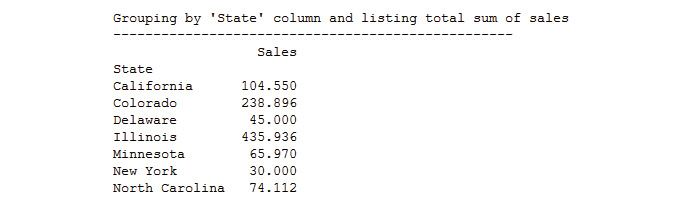
   Figure 4.17: The output after grouping the state with the listing sum of sales

5. Subset that DataFrame for a particular state and show the statistics:

   pd.DataFrame(byState.describe().loc['California'])

   The output is as follows:

   

   Figure 4.18: Checking the statistics of a particular state

6. Perform a similar summarization by using the Ship Mode attribute:

   df_subset.groupby('Ship Mode').describe().loc[['Second Class','Standard Class']]

   The output will be as follows:

   

   Figure 4.19: Checking the sales by summarizing the Ship Mode attribute

   Note how pandas has grouped the data by State first and then by cities under each state.

7. Display the complete summary statistics of sales by every city in each state – all by two lines of code by using the following command:

   byStateCity=df.groupby(['State','City'])

   byStateCity.describe()['Sales']

   The output is as follows:

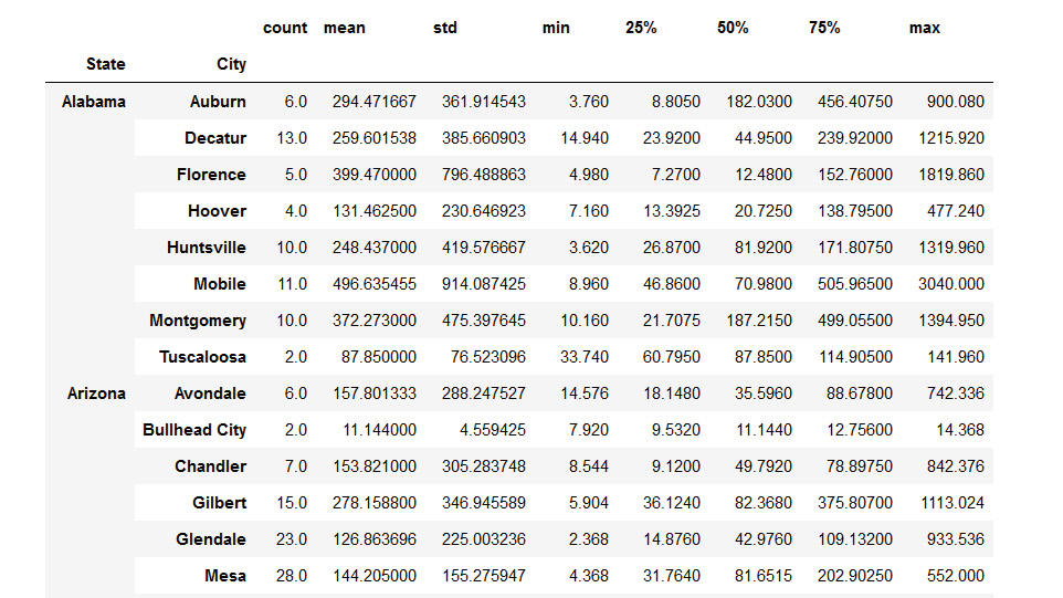
Figure 4.20: Checking the summary statistics of sales

Detecting Outliers and Handling Missing Values

Outlier detection and handling missing values fall under the subtle art of data quality checking. A modeling or data mining process is fundamentally a complex series of computations whose output quality largely depends on the quality and consistency of the input data being fed. The responsibility of maintaining and gate keeping that quality often falls on the shoulders of a data wrangling team.

Apart from the obvious issue of poor quality data, missing data can sometimes wreak havoc with the machine learning (ML) model downstream. A few ML models, like Bayesian learning, are inherently robust to outliers and missing data, but commonly techniques like Decision Trees and Random Forest have an issue with missing data because the fundamental splitting strategy employed by these techniques depends on an individual piece of data and not a cluster. Therefore, it is almost always imperative to impute missing data before handing it over to such a ML model.

Outlier detection is a subtle art. Often, there is no universally agreed definition of an outlier. In a statistical sense, a data point that falls outside a certain range may often be classified as an outlier, but to apply that definition, you need to have a fairly high degree of certainty about the assumption of the nature and parameters of the inherent statistical distribution about the data. It takes a lot of data to build that statistical certainty and even after that, an outlier may not be just an unimportant noise but a clue to something deeper. Let's take an example with some fictitious sales data from an American fast food chain restaurant. If we want to model the daily sales data as a time series, we observe an unusual spike in the data somewhere around mid-April:

Figure 4.21: Fictitious sales data of an American fast food chain restaurant

A good data scientist or data wrangler should develop curiosity about this data point rather than just rejecting it just because it falls outside the statistical range. In the actual anecdote, the sales figure really spiked that day because of an unusual reason. So, the data was real. But just because it was real does not mean it is useful. In the final goal of building a smoothly varying time series model, this one point should not matter and should be rejected. But the chapter here is that we cannot reject outliers without paying some attention to them.

Therefore, the key to outliers is their systematic and timely detection in an incoming stream of millions of data or while reading data from a cloud-based storage. In this topic, we will quickly go over some basic statistical tests for detecting outliers and some basic imputation techniques for filling up missing data.

Missing Values in Pandas

One of the most useful functions to detect missing values is isnull. Here, we have a snapshot of a DataFrame called df_missing (sampled partially from the superstore DataFrame we are working with) with some missing values:

Figure 4.22: DataFrame with missing values

Now, if we simply run the following code, we will get a DataFrame that's the same size as the original with boolean values as TRUE for the places where a NaN was encountered. Therefore, it is simple to test for the presence of any NaN/missing value for any row or column of the DataFrame. You just have to add the particular row and column of this boolean DataFrame. If the result is greater than zero, then you know there are some TRUE values (because FALSE here is denoted by 0 and TRUE here is denoted by 1) and correspondingly some missing values. Try the following snippet:

df_missing=pd.read_excel("Sample - Superstore.xls",sheet_name="Missing")

df_missing

The output is as follows:

Figure 4.23: DataFrame with the Excel values

Use the isnull function on the DataFrame and observe the results:

df_missing.isnull()

Figure 4.24 Output highlighting the missing values

Here is an example of some very simple code to detect, count, and print out missing values in every column of a DataFrame:

for c in df_missing.columns:

miss = df_missing[c].isnull().sum()

if miss>0:

print("{} has {} missing value(s)".format(c,miss))

else:

print("{} has NO missing value!".format(c))

This code scans every column of the DataFrame, calls the isnull function, and sums up the returned object (a pandas Series object, in this case) to count the number of missing values. If the missing value is greater than zero, it prints out the message accordingly. The output looks as follows:

Figure 4.25: Output of counting the missing values

Exercise 52: Filling in the Missing Values with fillna

To handle missing values, you should first look for ways not to drop them altogether but to fill them somehow. The fillna method is a useful function for performing this task on pandas DataFrames. The fillna method may work for string data, but not for numerical columns like sales or profits. So, we should restrict ourselves in regards to this fixed string replacement to non-numeric text-based columns only. The Pad or ffill function is used to fill forward the data, that is, copy it from the preceding data of the series.

The mean function can be used to fill using the average of the two values:

1. Fill all missing values with the string FILL by using the following command:

   df_missing.fillna('FILL')

   The output is as follows:

   

   Figure 4.26: Missing values replaced with FILL

2. Fill in the specified columns with the string FILL by using the following command:

   df_missing[['Customer','Product']].fillna('FILL')

   The output is as follows:

   

   Figure 4.27: Specified columns replaced with FILL

   Note

   In all of these cases, the function works on a copy of the original DataFrame. So, if you want to make the changes permanent, you have to assign the DataFrames that are returned by these functions to the original DataFrame object.

3. Fill in the values using pad or backfill by using the following command:

   df_missing['Sales'].fillna(method='ffill')

4. Use backfill or bfill to fill backward, that is, copy from the next data in the series:

   df_missing['Sales'].fillna(method='bfill')

   

   Figure 4.28: Using forward fill and backward fill to fill in missing data

5. You can also fill by using a function average of DataFrames. For example, we may want to fill the missing values in Sales by the average sales amount. Here is how we can do that:

   df_missing['Sales'].fillna(df_missing.mean()['Sales'])

Figure 4.29: Using average to fill in missing data

Exercise 53: Dropping Missing Values with dropna

This function is used to simply drop the rows or columns that contain NaN/missing values. However, there is some choice involved.

If the axis parameter is set to zero, then rows containing missing values are dropped; if the axis parameter is set to one, then columns containing missing values are dropped. These are useful if we don't want to drop a particular row/column if the NaN values do not exceed a certain percentage.

Two arguments that are useful for the dropna() method are as follows:

• The how argument determines if a row or column is removed from a DataFrame, when we have at least one NaN or all NaNs
• The thresh argument requires that many non-NaN values to keep the row/column

1. To set the axis parameter to zero and drop all missing rows, use the following command:

   df_missing.dropna(axis=0)

2. To set the axis parameter to one and drop all missing rows, use the following command:

   df_missing.dropna(axis=1)

   

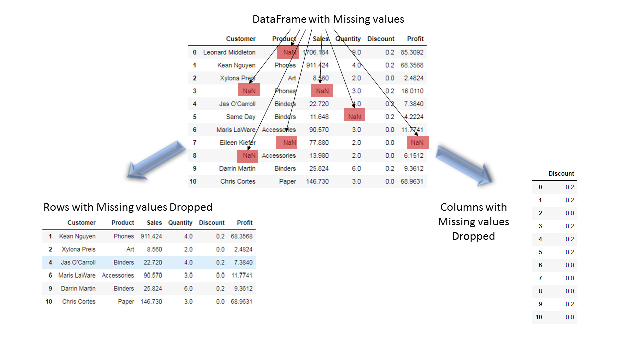
   Figure 4.30: Dropping rows or columns to handle missing data

3. Drop the values with the axis set to one and thresh set to 10:

   df_missing.dropna(axis=1,thresh=10)

   The output is as follows:

Figure 4.31: DataFrame with values dropped with axis=1 and thresh=10

All of these methods work on a temporary copy. To make a permanent change, you have to set inplace=True or assign the result to the original DataFrame, that is, overwrite it.

Outlier Detection Using a Simple Statistical Test

As we've already discussed, outliers in a dataset can occur due to many factors and in many ways:

• Data entry errors
• Experimental errors (data extraction related)
• Measurement errors due to noise or instrumental failure
• Data processing errors (data manipulation or mutations due to coding error)
• Sampling errors (extracting or mixing data from wrong or various sources)

It is impossible to pin-point one universal method for outlier detection. Here, we will show you some simple tricks for numeric data using standard statistical tests.

Boxplots may show unusual values. Corrupt two sales values by assigning negative, as follows:

df_sample = df[['Customer Name','State','Sales','Profit']].sample(n=50).copy()

df_sample['Sales'].iloc[5]=-1000.0

df_sample['Sales'].iloc[15]=-500.0

To plot the boxplot, use the following code:

df_sample.plot.box()

plt.title("Boxplot of sales and profit", fontsize=15)

plt.xticks(fontsize=15)

plt.yticks(fontsize=15)

plt.grid(True)

The output is as follows:

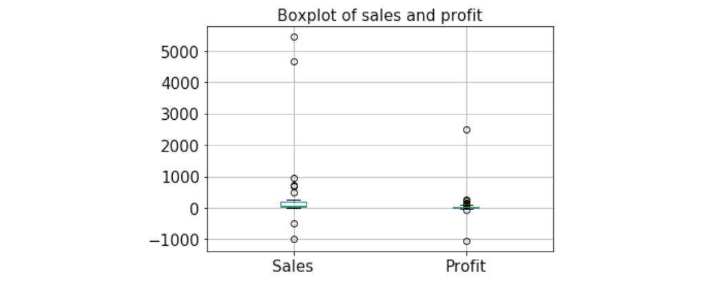
Figure 4.32: Boxplot of sales and profit

We can create simple boxplots to check for any unusual/nonsensical values. For example, in the preceding example, we intentionally corrupted two sales values to be negative and they were readily caught in a boxplot.

Note that profit may be negative, so those negative points are generally not suspicious. But sales cannot be negative in general, so they are detected as outliers.

We can create a distribution of a numerical quantity and check for values that lie at the extreme end to see if they are truly part of the data or outlier. For example, if a distribution is almost normal, then any value more than 4 or 5 standard deviations away may be a suspect:

Figure 4.33: Value away from the main outliers

Concatenating, Merging, and Joining

Merging and joining tables or datasets are highly common operations in the day-to-day job of a data wrangling professional. These operations are akin to the JOIN query in SQL for relational database tables. Often, the key data is present in multiple tables, and those records need to be brought into one combined table that's matching on that common key. This is an extremely common operation in any type of sales or transactional data, and therefore must be mastered by a data wrangler. The pandas library offers nice and intuitive built-in methods to perform various types of JOIN queries involving multiple DataFrame objects.

Exercise 54: Concatenation

We will start by learning the concatenation of DataFrames along various axes (rows or columns). This is a very useful operation as it allows you to grow a DataFrame as the new data comes in or new feature columns need to be inserted in the table:

1. Sample 4 records each to create three DataFrames at random from the original sales dataset we are working with:

   df_1 = df[['Customer Name','State','Sales','Profit']].sample(n=4)

   df_2 = df[['Customer Name','State','Sales','Profit']].sample(n=4)

   df_3 = df[['Customer Name','State','Sales','Profit']].sample(n=4)

2. Create a combined DataFrame with all the rows concatenated by using the following code:

   df_cat1 = pd.concat([df_1,df_2,df_3], axis=0)

   df_cat1

   

   Figure 4.34: Concatenating DataFrames together

3. You can also try concatenating along the columns, although that does not make any practical sense for this particular example. However, pandas fills in the unavailable values with NaN for that operation:

   df_cat2 = pd.concat([df_1,df_2,df_3], axis=1)

   df_cat2

Figure 4.35: Output after concatenating the DataFrames

Exercise 55: Merging by a Common Key

Merging by a common key is an extremely common operation for data tables as it allows you to rationalize multiple sources of data in one master database – that is, if they have some common features/keys.

This is often the first step in building a large database for machine learning tasks where daily incoming data may be put into separate tables. However, at the end of the day, the most recent table needs to be merged with the master data table to be fed into the backend machine learning server, which will then update the model and its prediction capacity.

Here, we will show a simple example of an inner join with Customer Name as the key:

1. One DataFrame, df_1, had shipping information associated with the customer name, and another table, df_2, had the product information tabulated. Our goal is to merge these tables into one DataFrame on the common customer name:

   df_1=df[['Ship Date','Ship Mode','Customer Name']][0:4]

   df_1

   The output is as follows:

   

   Figure 4.36: Entries in table df_1

   The second DataFrame is as follows:

   df_2=df[['Customer Name','Product Name','Quantity']][0:4]

   df_2

   The output is as follows:

   

   Figure 4.37: Entries in table df_2

2. Join these two tables by inner join by using the following command:

   pd.merge(df_1,df_2,on='Customer Name',how='inner')

   The output is as follows:

   

   Figure 4.38: Inner join on table df_1 and table df_2

3. Drop the duplicates by using the following command.

   pd.merge(df_1,df_2,on='Customer Name',how='inner').drop_duplicates()

   The output is as follows:

   

   Figure 4.39: Inner join on table df_1 and table df_2 after dropping the duplicates

4. Extract another small table called df_3 to show the concept of an outer join:

   df_3=df[['Customer Name','Product Name','Quantity']][2:6]

   df_3

   The output is as follows:

   

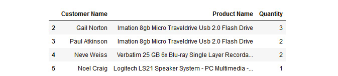
   Figure 4.40: Creating table df_3

5. Perform an inner join on df_1 and df_3 by using the following command:

   pd.merge(df_1,df_3,on='Customer Name',how='inner').drop_duplicates()

   The output is as follows:

   

   Figure 4.41: Merging table df_1 and table df_3 and dropping duplicates

6. Perform an outer join on df_1 and df_3 by using the following command:

   pd.merge(df_1,df_3,on='Customer Name',how='outer').drop_duplicates()

   The output is as follows:

Figure 4.42: Outer join on table df_1 and table df_2 and dropping the duplicates

Notice how some NaN and NaT values are inserted automatically because no corresponding entries could be found for those records, as those are the entries with unique customer names from their respective tables. NaT represents a Not a Time object, as the objects in the Ship Date column are of the nature of Timestamp objects.

Exercise 56: The join Method

Joining is performed based on index keys and is done by combining the columns of two potentially differently indexed DataFrames into a single one. It offers a faster way to accomplish merging by row indices. This is useful if the records in different tables are indexed differently but represent the same inherent data and you want to merge them into a single table:

1. Create the following tables with customer name as the index by using the following command:

   df_1=df[['Customer Name','Ship Date','Ship Mode']][0:4]

   df_1.set_index(['Customer Name'],inplace=True)

   df_1

   df_2=df[['Customer Name','Product Name','Quantity']][2:6]

   df_2.set_index(['Customer Name'],inplace=True)

   df_2

   The outputs is as follows:

   

   Figure 4.43: DataFrames df_1 and df_2

2. Perform a left join on df_1 and df_2 by using the following command:

   df_1.join(df_2,how='left').drop_duplicates()

   The output is as follows:

   

   Figure 4.44: Left join on table df_1 and table df_2 after dropping the duplicates

3. Perform a right join on df_1 and df_2 by using the following command:

   df_1.join(df_2,how='right').drop_duplicates()

   The output is as follows:

   

   Figure 4.45: Right join on table df_1 and table df_2 after dropping the duplicates

4. Perform an inner join on df_1 and df_2 by using the following command:

   df_1.join(df_2,how='inner').drop_duplicates()

   The output is as follows:

   

   Figure 4.46: Inner join on table df_1 and table df_2 after dropping the duplicates

5. Perform an outer join on df_1 and df_2 by using the following command:

   df_1.join(df_2,how='outer').drop_duplicates()

   The output is as follows:

Figure 4.47: Outer join on table df_1 and table df_2 after dropping the duplicates

Useful Methods of Pandas

In this topic, we will discuss some small utility functions that are offered by pandas so that we can work efficiently with DataFrames. They don't fall under any particular group of function, so they are mentioned here under the Miscellaneous category.

Exercise 57: Randomized Sampling

Sampling a random fraction of a big DataFrame is often very useful so that we can practice other methods on them and test our ideas. If you have a database table of 1 million records, then it is not computationally effective to run your test scripts on the full table.

However, you may also not want to extract only the first 100 elements as the data may have been sorted by a particular key and you may get an uninteresting table back, which may not represent the full statistical diversity of the parent database.

In these situations, the sample method comes in super handy so that we can randomly choose a controlled fraction of the DataFrame:

1. Specify the number of samples that you require from the DataFrame by using the following command:

   df.sample(n=5)

   The output is as follows:

   

   Figure 4.48: DataFrame with 5 samples

2. Specify a definite fraction (percentage) of data to be sampled by using the following command:

   df.sample(frac=0.1)

   The output is as follows:

   

   Figure 4.49: DataFrame with 0.1% data sampled

   You can also choose if sampling is done with replacement, that is, whether the same record can be chosen more than once. The default replace choice is FALSE, that is, no repetition, and sampling will try to choose new elements only.

3. Choose the sampling by using the following command:

   df.sample(frac=0.1, replace=True)

   The output is as follows:

Figure 4.50: DataFrame with 0.1% data sampled and repetition enabled

The value_counts Method

We discussed the unique method before, which finds and counts the unique records from a DataFrame. Another useful function in a similar vein is value_counts. This function returns an object containing counts of unique values. In the object that is returned, the first element is the most frequently used object. The elements are arranged in descending order.

Let's consider a practical application of this method to illustrate the utility. Suppose your manager asks you to list the top 10 customers from the big sales database that you have. So, the business question is: which 10 customers' names occur the most frequently in the sales table? You can achieve the same with an SQL query if the data is in a RDBMS, but in pandas, this can be done by using one simple function:

df['Customer Name'].value_counts()[:10]

The output is as follows:

Figure 4.51: List of top 10 customers

The value_counts method returns a series of the counts of all unique customer names sorted by the frequency of the count. By asking for only the first 10 elements of that list, this code returns a series of the most frequently occurring top 10 customer names.

Pivot Table Functionality

Similar to group by, pandas also offer pivot table functionality, which works the same as a pivot table in spreadsheet programs like MS Excel. For example, in this sales database, you want to know the average sales, profit, and quantity sold, by Region and State (two levels of index).

We can extract this information by using one simple piece of code (we sample 100 records first for keeping the computation fast and then apply the code):

df_sample = df.sample(n=100)

df_sample.pivot_table(values=['Sales','Quantity','Profit'],index=['Region','State'],aggfunc='mean')

The output is as follows (note that your specific output may be different due to random sampling):

Figure 4.52: Sample of 100 records

Exercise 58: Sorting by Column Values – the sort_values Method

Sorting a table by a particular column is one of the most frequently used operations in the daily work of an analyst. Not surprisingly, pandas provide a simple and intuitive method for sorting called the sort_values method:

1. Take a random sample of 15 records and then show how we can sort by the Sales column and then by both the Sales and State columns together:

   df_sample=df[['Customer Name','State','Sales','Quantity']].sample(n=15)

   df_sample

   The output is as follows:

   

   Figure 4.53: Sample of 15 records

2. Sort the values with respect to Sales by using the following command:

   df_sample.sort_values(by='Sales')

   The output is as follows:

   

   Figure 4.54: DataFrame with the Sales value sorted

3. Sort the values with respect to Sales and State:

   df_sample.sort_values(by=['State','Sales'])

   The output is as follows:

Figure 4.55: DataFrame sorted with respect to Sales and State

Exercise 59: Flexibility for User-Defined Functions with the apply Method

The pandas library provides great flexibility to work with user-defined functions of arbitrary complexity through the apply method. Much like the native Python apply function, this method accepts a user-defined function and additional arguments and returns a new column after applying the function on a particular column element-wise.

As an example, suppose we want to create a column of categorical features like high/medium/low based on the sales price column. Note that it is a conversion from a numeric value to a categorical factor (string) based on certain conditions (threshold values of sales):

1. Create a user-defined function, as follows:

   def categorize_sales(price):

   if price < 50:

   return "Low"

   elif price < 200:

   return "Medium"

   else:

   return "High"

2. Sample 100 records randomly from the database:

   df_sample=df[['Customer Name','State','Sales']].sample(n=100)

   df_sample.head(10)

   The output is as follows:

   

   Figure 4.56: 100 sample records from the database

3. Use the apply method to apply the categorization function onto the Sales column:

   Note

   We need to create a new column to store the category string values that are returned by the function.

   df_sample['Sales Price Category']=df_sample['Sales'].apply(categorize_sales)

   df_sample.head(10)

   The output is as follows:

   

   Figure 4.57: DataFrame with 10 rows after using the apply function on the Sales column

4. The apply method also works with the built-in native Python functions. For practice, let's create another column for storing the length of the name of the customer. We can do that using the familiar len function:

   df_sample['Customer Name Length']=df_sample['Customer Name'].apply(len)

   df_sample.head(10)

   The output is as follows:

   

   Figure 4.58: DataFrame with a new column

5. Instead of writing out a separate function, we can even insert lambda expressions directly into the apply method for short functions. For example, let's say we are promoting our product and want to show the discounted sales price if the original price is > $200. We can do this using a lambda function and the apply method:

   df_sample['Discounted Price']=df_sample['Sales'].apply(lambda x:0.85*x if x>200 else x)

   df_sample.head(10)

   The output is as follows:

Figure 4.59: Lambda function

Note

The lambda function contains a conditional, and a discount is applied to those records where the original sales price is > $200.

Activity 6: Working with the Adult Income Dataset (UCI)

In this activity, you will work with the Adult Income Dataset from the UCI machine learning portal. The Adult Income dataset has been used in many machine learning papers that address classification problems. You will read the data from a CSV file into a pandas DataFrame and do some practice on the advanced data wrangling you learned about in this chapter.

The aim of this activity is to practice various advanced pandas DataFrame operations, for example, for subsetting, applying user-defined functions, summary statistics, visualizations, boolean indexing, group by, and outlier detection on a real-life dataset. We have the data downloaded as a CSV file on the disk for your ease. However, it is recommended to practice data downloading on your own so that you are familiar with the process.

Here is the URL for the dataset: https://archive.ics.uci.edu/ml/machine-learning-databases/adult/.

Here is the URL for the description of the dataset and the variables: https://archive.ics.uci.edu/ml/machine-learning-databases/adult/adult.names.

These are the steps that will help you solve this activity:

1. Load the necessary libraries.
2. Read the adult income dataset from the following URL: https://github.com/TrainingByPackt/Data-Wrangling-with-Python/blob/master/Chapter04/Activity06/.
3. Create a script that will read a text file line by line.
4. Add a name of Income for the response variable to the dataset.
5. Find the missing values.
6. Create a DataFrame with only age, education, and occupation by using subsetting.
7. Plot a histogram of age with a bin size of 20.
8. Create a function to strip the whitespace characters.
9. Use the apply method to apply this function to all the columns with string values, create a new column, copy the values from this new column to the old column, and drop the new column.
10. Find the number of people who are aged between 30 and 50.
11. Group the records based on age and education to find how the mean age is distributed.
12. Group by occupation and show the summary statistics of age. Find which profession has the oldest workers on average and which profession has its largest share of the workforce above the 75th percentile.
13. Use subset and groupby to find outliers.
14. Plot the values on a bar chart.
15. Merge the data using common keys.

    Note

    The solution for this activity can be found on page 297.

Summary

In this chapter, we dived deep into the pandas library to learn advanced data wrangling techniques. We started with some advanced subsetting and filtering on DataFrames and round this up by learning about boolean indexing and conditional selection of a subset of data. We also covered how to set and reset the index of a DataFrame, especially while initializing.

Next, we learned about a particular topic that has a deep connection with traditional relational database systems – the group by method. Then, we dived deep into an important skill for data wrangling - checking for and handling missing data. We showed you how pandas help in handling missing data using various imputation techniques. We also discussed methods for dropping missing values. Furthermore, methods and usage examples of concatenation and merging of DataFrame objects were shown. We saw the join method and how it compares to a similar operation in SQL.

Lastly, miscellaneous useful methods on DataFrames, such as randomized sampling, unique, value_count, sort_values, and pivot table functionality were covered. We also showed an example of running an arbitrary user-defined function on a DataFrame using the apply method.

After learning about the basic and advanced data wrangling techniques with NumPy and pandas libraries, the natural question of data acquiring rises. In the next chapter, we will show you how to work with a wide variety of data sources, that is, you will learn how to read data in tabular format in pandas from different sources.