Chapter 8

RDBMS and SQL

Learning Objectives

By the end of this chapter, you will be able to:

• Apply the basics of RDBMS to query databases using Python
• Convert data from SQL into a pandas DataFrame

This chapter explains the concepts of databases, including their creation, manipulation and control, and transforming tables into pandas DataFrames.

Introduction

This chapter of our data journey is focused on RDBMS (Relational Database Management Systems) and SQL (Structured Query Language). In the previous chapter, we stored and read data from a file. In this chapter, we will read structured data, design access to the data, and create query interfaces for databases.

Data has been stored in RDBMS format for years. The reasons behind it are as follows:

• RDBMS is one of the safest ways to store, manage, and retrieve data.
• They are backed by a solid mathematical foundation (relational algebra and calculus) and they expose an efficient and intuitive declarative language – SQL – for easy interaction.
• Almost every language has a rich set of libraries to interact with different RDBMS and the tricks and methods of using them are well tested and well understood.
• Scaling an RDBMS is a pretty well-understood task and there are a bunch of well trained, experienced professionals to do this job (DBA or database administrator).

As we can see in the following chart, the market of DBMS is big. This chart was produced based on market research that was done by Gartner, Inc. in 2016:

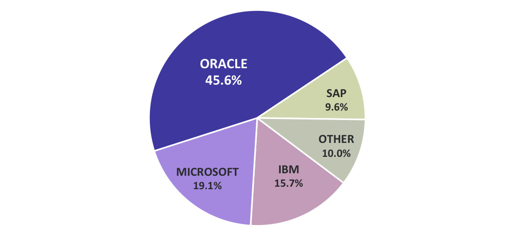
Figure 8.1 Commercial database market share in 2016

We will learn and play around with some basic and fundamental concepts of database and database management systems in this chapter.

Refresher of RDBMS and SQL

An RDBMS is a piece of software that manages data (represented for the end user in a tabular form) on physical hard disks and is built using the Codd's relational model. Most of the databases that we encounter today are RDBMS. In recent years, there has been a huge industry shift toward a newer kind of database management system, called NoSQL (MongoDB, CouchDB, Riak, and so on). These systems, although in some aspects they follow some of the rules of RDBMS, in most cases reject or modify them.

How is an RDBMS Structured?

The RDBMS structure consists of three main elements, namely the storage engine, query engine, and log management. Here is a diagram that shows the structure of a RDBMS:

Figure 8.2 RDBMS structure

The following are the main concepts of any RDBMS structure:

• Storage engine: This is the part of the RDBMS that is responsible for storing the data in an efficient way and also to give it back when asked for, in an efficient way. As an end user of the RDBMS system (an application developer is considered an end user of an RDBMS), we will never need to interact with this layer directly.
• Query engine: This is the part of the RDBMS that allows us to create data objects (tables, views, and so on), manipulate them (create and delete columns, create/delete/update rows, and so on), and query them (read rows) using a simple yet powerful language.
• Log management: This part of the RDBMS is responsible for creating and maintaining the logs. If you are wondering why the log is such an important thing, then you should look into how replication and partitions are handled in a modern RDBMS (such as PostgreSQL) using something called Write Ahead Log (or WAL for short).

We will focus on the query engine in this chapter.

SQL

Structured Query Language or SQL (pronounced sequel), as it is commonly known, is a domain-specific language that was originally designed based on E.F. Codd's relational model and is widely used in today's databases to define, insert, manipulate, and retrieve data from them. It can be further sub-divided into four smaller sub-languages, namely DDL (Data Definition Language), DML (Data Manipulation Language), DQL (Data Query Language), and DCL (Data Control Language). There are several advantages of using SQL, with some of them being as follows:

• It is based on a solid mathematical framework and thus it is easy to understand.
• It is a declarative language, which means that we actually never tell it how to do its job. We almost always tell it what to do. This frees us from a big burden of writing custom code for data management. We can be more focused on the actual query problem we are trying to solve instead of bothering about how to create and maintain a data store.
• It gives you a fast and readable way to deal with data.
• SQL gives you out-of-the-box ways to get multiple pieces of data with a single query.

The main areas of focus for the following topic will be DDL, DML, and DQL. The DCL part is more for database administrators.

• DDL: This is how we define our data structure in SQL. As RDBMS is mainly designed and built with structured data in mind, we have to tell an RDBMS engine beforehand what our data is going to look like. We can update this definition at a later point in time, but an initial one is a must. This is where we will write statements such as CREATE TABLE or DROP TABLE or ALTER TABLE.

  Note

  Notice the use of uppercase letters. It is not a specification and you can use lowercase letters, but it is a widely followed convention and we will use that in this book.

• DML: DML is the part of SQL that let us insert, delete, or update a certain data point (a row) in a previously defined data object (a table). This is the part of SQL which contains statements such as INSERT INTO, DELETE FROM, or UPDATE.
• DQL: With DQL, we enable ourselves to query the data stored in a RDBMS, which was defined by DDL and inserted using DML. It gives us enormous power and flexibility to not only query data out of a single object (table), but also to extract relevant data from all the related objects using queries. The frequently used query that's used to retrieve data is the SELECT command. We will also see and use the concepts of the primary key, foreign key, index, joins, and so on.

Once you define and insert data in a database, it can be represented as follows:

Figure 8.3 Table displaying sample data

Another thing to remember about RDBMS is relations. Generally, in a table, we have one or more columns that will have unique values for each row in the table. We call them primary keys for the table. We should be aware that we will encounter unique values across the rows, which are not primary keys. The main difference between them and primary keys is the fact that a primary key cannot be null.

By using the primary key of one table and mentioning it as a foreign key in another table, we can establish relations between two tables. A certain table can be related to any finite number of tables. The relations can be 1:1, which means that each row of the second table is uniquely related to one row of the first table, or 1 :N, N:1, or N: M. An example of relations is as follows:

Figure 8.4 Diagram showing relations

With this brief refresher, we are now ready to jump into hands-on exercises and write some SQL to store and retrieve data.

Using an RDBMS (MySQL/PostgreSQL/SQLite)

In this topic, we will focus on how to write some basic SQL commands, as well as how to connect to a database from Python and use it effectively within Python. The database we will choose here is SQLite. There are other databases, such as Oracle, MySQL, Postgresql, and DB2. The main tricks that you are going to learn here will not change based on what database you are using. But for different databases, you will need to install different third-party Python libraries (such as Psycopg2 for Postgresql, and so on). The reason they all behave the same way (apart for some small details) is the fact that they all adhere to PEP249 (commonly known as Python DB API 2).

This is a good standardization and saves us a lot of headaches while porting from one RDBMS to another.

Note

Most of the industry standard projects which are written in Python and use some kind of RDBMS as the data store, most often relay on an ORM or Object Relational Mapper. An ORM is a high-level library in Python which makes many tasks, while dealing with RDBMS, easier. It also exposes a more Pythonic API than writing raw SQL inside Python code.

Exercise 107: Connecting to Database in SQLite

In this exercise, we will look into the first step toward using a RDBMS in Python code. All we are going to do is connect to a database and then close the connection. We will also learn about the best way to do this:

1. Import the sqlite3 library of Python by using the following command:

   import sqlite3

2. Use the connect function to connect to a database. If you already have some experience with databases, then you will notice that we are not using any server address, user name, password, or other credentials to connect to a database. This is because these fields are not mandatory in sqlite3, unlike in Postgresql or MySQL. The main database engine of SQLite is embedded:

   conn = sqlite3.connect("chapter.db")

3. Close the connection, as follows:

   conn.close()

   This conn object is the main connection object, and we will need that to get a second type of object in the future once we want to interact with the database. We need to be careful about closing any open connection to our database.

4. Use the same with statement from Python, just like we did for files, and connect to the database, as follows:

   with sqlite3.connect("chapter.db") as conn:

   pass

In this exercise, we have connected to a database using Python.

Exercise 108: DDL and DML Commands in SQLite

In this exercise, we will look at how we can create a table, and we will also insert data in it.

As the name suggests, DDL (Data Definition Language) is the way to communicate to the database engine in advance to define what the data will look like. The database engine creates a table object based on the definition provided and prepares it.

To create a table in SQL, use the CREATE TABLE SQL clause. This will need the table name and the table definition. Table name is a unique identifier for the database engine to find and use the table for all future transactions. It can be anything (any alphanumeric string), as long as it is unique. We add the table definition in the form of (column_name_1 data_type, column_name_2 data type, … ). For our purpose, we will use the text and integer datatypes, but usually a standard database engine supports many more datatypes, such as float, double, date time, Boolean, and so on. We will also need to specify a primary key. A primary key is a unique, non-null identifier that's used to uniquely identify a row in a table. In our case, we use email as a primary key. A primary key can be an integer or text.

The last thing you need to know is that unless you call a commit on the series of operations you just performed (together, we formally call them a transaction), nothing will be actually performed and reflected in the database. This property is called atomicity. In fact, for a database to be industry standard (to be useable in real life), it needs to follow the ACID (Atomicity, Consistency, Isolation, Durability) properties:

1. Use SQLite's connect function to connect to the chapter.db database, as follows:

   with sqlite3.connect("chapter.db") as conn:

   Note

   This code will work once you add the snippet from step 3.

2. Create a cursor object by calling conn.cursor(). The cursor object acts as a medium to communicate with the database. Create a table in Python, as follows:

   cursor = conn.cursor()

   cursor.execute("CREATE TABLE IF NOT EXISTS user (email text, first_name text, last_name text, address text, age integer, PRIMARY KEY (email))")

3. Insert rows into the database that you created, as follows:

   cursor.execute("INSERT INTO user VALUES ('[email protected]', 'Bob', 'Codd', '123 Fantasy lane, Fantasy City', 31)")

   cursor.execute("INSERT INTO user VALUES ('[email protected]', 'Tom', 'Fake', '456 Fantasy lane, Fantasu City', 39)")

4. Commit to the database:

   conn.commit()

This will create the table and write two rows to it with data.

Reading Data from a Database in SQLite

In the preceding exercise, we created a table and stored data in it. Now, we will learn how to read the data that's stored in this database.

The SELECT clause is immensely powerful, and it is really important for a data practitioner to master SELECT and everything related to it (such as conditions, joins, group-by, and so on).

The * after SELECT tells the engine to select all of the columns from the table. It is a useful shorthand. We have not mentioned any condition for the selection (such as above a certain age, first name starting with a certain sequence of letters, and so on). We are practically telling the database engine to select all the rows and all the columns from the table. It is time-consuming and less effective if we have a huge table. Hence, we would want to use the LIMIT clause to limit the number of rows we want.

You can use the SELECT clause in SQL to retrieve data, as follows:

with sqlite3.connect("chapter.db") as conn:

cursor = conn.cursor()

rows = cursor.execute('SELECT * FROM user')

for row in rows:

print(row)

The output is as follows:

Figure 8.5: Output of the SELECT clause

The syntax to use the SELECT clause with a LIMIT as follows:

SELECT * FROM <table_name> LIMIT 50;

Note

This syntax is a sample code and will not work on Jupyter notebook.

This will select all the columns, but only the first 50 rows from the table.

Exercise 109: Sorting Values that are Present in the Database

In this exercise, we will use the ORDER BY clause to sort the rows of user table with respect to age:

1. Sort the chapter.db by age in descending order, as follows:

   with sqlite3.connect("chapter.db") as conn:

   cursor = conn.cursor()

   rows = cursor.execute('SELECT * FROM user ORDER BY age DESC')

   for row in rows:

   print(row)

   The output is as follows:

   

   Figure 8.6: Output of data displaying age in descending order

2. Sort the chapter.db by age in ascending order, as follows:

   with sqlite3.connect("chapter.db") as conn:

   cursor = conn.cursor()

   rows = cursor.execute('SELECT * FROM user ORDER BY age')

   for row in rows:

   print(row)

3. The output is as follows:

Figure 8.7: Output of data displaying age in ascending order

Notice that we don't need to specify the order as ASC to sort it into ascending order.

Exercise 110: Altering the Structure of a Table and Updating the New Fields

In this exercise, we are going to add a column using ALTER and UPDATE the values in the newly added column.

The UPDATE command is used to edit/update any row after it has been inserted. Be careful when using it because using UPDATE without selective clauses (such as WHERE) affects the entire table:

1. Establish the connection with the database by using the following command:

   with sqlite3.connect("chapter.db") as conn:

   cursor = conn.cursor()

2. Add another column in the user table and fill it with null values by using the following command:

   cursor.execute("ALTER TABLE user ADD COLUMN gender text")

3. Update all of the values of gender so that they are M by using the following command:

   cursor.execute("UPDATE user SET gender='M'")

   conn.commit()

4. To check the altered table, execute the following command:

   rows = cursor.execute('SELECT * FROM user')

   for row in rows:

   print(row)

Figure 8.8: Output after altering the table

We have updated the entire table by setting the gender of all the users as M, where M stands for male.

Exercise 111: Grouping Values in Tables

In this exercise, we will learn about a concept that we have already learned about in pandas. This is the GROUP BY clause. The GROUP BY clause is a technique that's used to retrieve distinct values from the database and place them in individual buckets.

The following diagram explains how the GROUP BY clause works:

Figure 8.9: Illustration of the GROUP BY clause on a table

In the preceding diagram, we can see that the Col3 column has only two unique values across all rows, A and B.

The command that's used to check the total number of rows belonging to each group is as follows:

SELECT count(*), col3 FROM table1 GROUP BY col3

Add female users to the table and group them based on the gender:

1. Add a female user to the table:

   cursor.execute("INSERT INTO user VALUES ('[email protected]', 'Shelly', 'Milar', '123, Ocean View Lane', 39, 'F')")

2. Run the following code to see the count by each gender:

   rows = cursor.execute("SELECT COUNT(*), gender FROM user GROUP BY gender")

   for row in rows:

   print(row)

   The output is as follows:

Figure 8.10: Output of the GROUP BY clause

Relation Mapping in Databases

We have been working with a single table and altering it, as well as reading back the data. However, the real power of an RDBMS comes from the handling of relationships among different objects (tables). In this section, we are going to create a new table called comments and link it with the user table in a 1: N relationship. This means that one user can have multiple comments. The way we are going to do this is by adding the user table's primary key as a foreign key in the comments table. This will create a 1: N relationship.

When we link two tables, we need to specify to the database engine what should be done if the parent row is deleted, which has many children in the other table. As we can see in the following diagram, we are asking what happens at the place of the question marks when we delete row1 of the user table:

Figure 8.11: Illustration of relations

In a non-RDBMS situation, this situation can quickly become difficult and messy to manage and maintain. However, with an RDBMS, all we have to tell the database engine, in very precise ways, is what to do when a situation like this occurs. The database engine will do the rest for us. We use ON DELETE to tell the engine what we do with all the rows of a table when the parent row gets deleted. The following code illustrates these concepts:

with sqlite3.connect("chapter.db") as conn:

cursor = conn.cursor()

cursor.execute("PRAGMA foreign_keys = 1")

sql = """

CREATE TABLE comments (

user_id text,

comments text,

FOREIGN KEY (user_id) REFERENCES user (email)

ON DELETE CASCADE ON UPDATE NO ACTION

)

"""

cursor.execute(sql)

conn.commit()

The ON DELETE CASCADE line informs the database engine that we want to delete all the children rows when the parent gets deleted. We can also define actions for UPDATE. In this case, there is nothing to do on UPDATE.

The FOREIGN KEY modifier modifies a column definition (user_id, in this case) and marks it as a foreign key, which is related to the primary key (email, in this case) of another table.

You may notice the strange looking cursor.execute("PRAGMA foreign_keys = 1") line in the code. It is there just because SQLite does not use the normal foreign key features by default. It is this line that enables that feature. It is typical to SQLite and we won't need it for any other databases.

Adding Rows in the comments Table

We have created a table called comments. In this section, we will dynamically generate an insert query, as follows:

with sqlite3.connect("chapter.db") as conn:

cursor = conn.cursor()

cursor.execute("PRAGMA foreign_keys = 1")

sql = "INSERT INTO comments VALUES ('{}', '{}')"

rows = cursor.execute('SELECT * FROM user ORDER BY age')

for row in rows:

email = row[0]

print("Going to create rows for {}".format(email))

name = row[1] + " " + row[2]

for i in range(10):

comment = "This is comment {} by {}".format(i, name)

conn.cursor().execute(sql.format(email, comment))

conn.commit()

Pay attention to how we dynamically generate the insert query so that we can insert 10 comments for each user.

Joins

In this exercise, we will learn how to exploit the relationship we just built. This means that if we have the primary key from one table, we can recover all the data needed from that table and also all the linked rows from the child table. To achieve this, we will use something called a join.

A join is basically a way to retrieve linked rows from two tables using any kind of primary key - foreign key relation that they have. There are many types of join, such as INNER, LEFT OUTER, RIGHT OUTER, FULL OUTER, and CROSS. They are used in different situations. However, most of the time, in simple 1: N relations, we end up using an INNER join. In Chapter 1: Introduction to Data Wrangling with Python, we learned about sets, then we can view an INNER JOIN as an intersection of two sets. The following diagram illustrate the concepts:

Figure 8.12: Intersection Join

Here, A represents one table and B represents another. The meaning of having common members is to have a relationship between them. It takes all of the rows of A and compares them with all of the rows of B to find the matching rows that satisfy the join predicate. This can quickly become a complex and time-consuming operation. Joins can be very expensive operations. Usually, we use some kind of where clause, after we specify the join, to shorten the scope of rows that are fetched from table A or B to perform the matching.

In our case, our first table, user, has three entries, with the primary key being the email. We can make use of this in our query to get comments just from Bob:

with sqlite3.connect("chapter.db") as conn:

cursor = conn.cursor()s

cursor.execute("PRAGMA foreign_keys = 1")

sql = """

SELECT * FROM comments

JOIN user ON comments.user_id = user.email

WHERE user.email='[email protected]'

"""

rows = cursor.execute(sql)

for row in rows:

print(row)

The output is as follows:

('[email protected]', 'This is comment 0 by Bob Codd', '[email protected]', 'Bob', 'Codd', '123 Fantasy lane, Fantasu City', 31, None)

('[email protected]', 'This is comment 1 by Bob Codd', '[email protected]', 'Bob', 'Codd', '123 Fantasy lane, Fantasu City', 31, None)

('[email protected]', 'This is comment 2 by Bob Codd', '[email protected]', 'Bob', 'Codd', '123 Fantasy lane, Fantasu City', 31, None)

('[email protected]', 'This is comment 3 by Bob Codd', '[email protected]', 'Bob', 'Codd', '123 Fantasy lane, Fantasu City', 31, None)

('[email protected]', 'This is comment 4 by Bob Codd', '[email protected]', 'Bob', 'Codd', '123 Fantasy lane, Fantasu City', 31, None)

('[email protected]', 'This is comment 5 by Bob Codd', '[email protected]', 'Bob', 'Codd', '123 Fantasy lane, Fantasu City', 31, None)

('[email protected]', 'This is comment 6 by Bob Codd', '[email protected]', 'Bob', 'Codd', '123 Fantasy lane, Fantasu City', 31, None)

('[email protected]', 'This is comment 7 by Bob Codd', '[email protected]', 'Bob', 'Codd', '123 Fantasy lane, Fantasu City', 31, None)

('[email protected]', 'This is comment 8 by Bob Codd', '[email protected]', 'Bob', 'Codd', '123 Fantasy lane, Fantasu City', 31, None)

('[email protected]', 'This is comment 9 by Bob Codd', '[email protected]', 'Bob', 'Codd', '123 Fantasy lane, Fantasu City', 31, None)

Figure 8.13: Output of the Join query

Retrieving Specific Columns from a JOIN query

In the previous exercise, we saw that we can use a JOIN to fetch the related rows from two tables. However, if we look at the results, we will see that it returned all the columns, thus combining both tables. This is not very concise. What about if we only want to see the emails and the related comments, and not all the data?

There is some nice shorthand code that lets us do this:

with sqlite3.connect("chapter.db") as conn:

cursor = conn.cursor()

cursor.execute("PRAGMA foreign_keys = 1")

sql = """

SELECT comments.* FROM comments

JOIN user ON comments.user_id = user.email

WHERE user.email='[email protected]'

"""

rows = cursor.execute(sql)

for row in rows:

print(row)

Just by changing the SELECT statement, we made our final result look as follows:

('[email protected]', 'This is comment 0 by Bob Codd')

('[email protected]', 'This is comment 1 by Bob Codd')

('[email protected]', 'This is comment 2 by Bob Codd')

('[email protected]', 'This is comment 3 by Bob Codd')

('[email protected]', 'This is comment 4 by Bob Codd')

('[email protected]', 'This is comment 5 by Bob Codd')

('[email protected]', 'This is comment 6 by Bob Codd')

('[email protected]', 'This is comment 7 by Bob Codd')

('[email protected]', 'This is comment 8 by Bob Codd')

('[email protected]', 'This is comment 9 by Bob Codd')

Exercise 112: Deleting Rows

In this exercise, we are going to delete a row from the user table and observe the effects it will have on the comments table. Be very careful when running this command as it can have a destructive effect on the data. Please keep in mind that it has to almost always be run accompanied by a WHERE clause so that we delete just a part of the data and not everything:

1. To delete a row from a table, we use the DELETE clause in SQL. To run delete on the user table, we are going to use the following code:

   with sqlite3.connect("chapter.db") as conn:

   cursor = conn.cursor()

   cursor.execute("PRAGMA foreign_keys = 1")

   cursor.execute("DELETE FROM user WHERE email='[email protected]'")

   conn.commit()

2. Perform the SELECT operation on the user table:

   with sqlite3.connect("chapter.db") as conn:

   cursor = conn.cursor()

   cursor.execute("PRAGMA foreign_keys = 1")

   rows = cursor.execute("SELECT * FROM user")

   for row in rows:

   print(row)

   Observe that the user Bob has been deleted.

   Now, moving on to the comments table, we have to remember that we had mentioned ON DELETE CASCADE while creating the table. The database engine knows that if a row is deleted from the parent table (user), all the related rows from the child tables (comments) will have to be deleted.

3. Perform a select operation on the comments table by using the following command:

   with sqlite3.connect("chapter.db") as conn:

   cursor = conn.cursor()

   cursor.execute("PRAGMA foreign_keys = 1")

   rows = cursor.execute("SELECT * FROM comments")

   for row in rows:

   print(row)

   The output is as follows:

   ('[email protected]', 'This is comment 0 by Tom Fake')

   ('[email protected]', 'This is comment 1 by Tom Fake')

   ('[email protected]', 'This is comment 2 by Tom Fake')

   ('[email protected]', 'This is comment 3 by Tom Fake')

   ('[email protected]', 'This is comment 4 by Tom Fake')

   ('[email protected]', 'This is comment 5 by Tom Fake')

   ('[email protected]', 'This is comment 6 by Tom Fake')

   ('[email protected]', 'This is comment 7 by Tom Fake')

   ('[email protected]', 'This is comment 8 by Tom Fake')

   ('[email protected]', 'This is comment 9 by Tom Fake')

   We can see that all of the rows related to Bob are deleted.

Updating Specific Values in a Table

In this exercise, we will see how we can update rows in a table. We have already looked at this in the past but, as we mentioned, at a table level only. Without WHERE, updating is often a bad idea.

Combine UPDATE with WHERE to selectively update the first name of the user with the email address [email protected]:

with sqlite3.connect("chapter.db") as conn:

cursor = conn.cursor()

cursor.execute("PRAGMA foreign_keys = 1")

cursor.execute("UPDATE user set first_name='Chris' where email='[email protected]'")

conn.commit()

rows = cursor.execute("SELECT * FROM user")

for row in rows:

print(row)

The output is as follows:

Figure 8.14: Output of the update query

Exercise 113: RDBMS and DataFrames

We have looked into many fundamental aspects of storing and querying data from a database, but as a data wrangling expert, we need our data to be packed and presented as a DataFrame so that we can perform quick and convenient operations on them:

1. Import pandas using the following code:

   import pandas as pd

2. Create a columns list with email, first name, last name, age, gender, and comments as column names. Also, create an empty data list:

   columns = ["Email", "First Name", "Last Name", "Age", "Gender", "Comments"]

   data = []

3. Connect to chapter.db using SQLite and obtain a cursor, as follows:

   with sqlite3.connect("chapter.db") as conn:

   cursor = conn.cursor()

   Use the execute method from the cursor to set "PRAGMA foreign_keys = 1"

   cursor.execute("PRAGMA foreign_keys = 1")

4. Create a sql variable that will contain the SELECT command and use the join command to join the databases:

   sql = """

   SELECT user.email, user.first_name, user.last_name, user.age, user.gender, comments.comments FROM comments

   JOIN user ON comments.user_id = user.email

   WHERE user.email = '[email protected]'

   """

5. Use the execute method of cursor to execute the sql command:

   rows = cursor.execute(sql)

6. Append the rows to the data list:

   for row in rows:

   data.append(row)

7. Create a DataFrame using the data list:

   df = pd.DataFrame(data, columns=columns)

8. We have created the DataFrame using the data list. You can print the values into the DataFrame using df.head.

Activity 11: Retrieving Data Correctly From Databases

In this activity, we have the persons table:

Figure 8.15: The persons table

We have the pets table:

Figure 8.16: The pets table

As we can see, the id column in the persons table (which is an integer) serves as the primary key for that table and as a foreign key for the pet table, which is linked via the owner_id column.

The persons table has the following columns:

• first_name: The first name of the person
• last_name: The last name of the person (can be "null")
• age: The age of the person
• city: The city from where he/she is from
• zip_code: The zip code of the city

The pets table has the following columns:

• pet_name: The name of the pet.
• pet_type: What type of pet it is, for example, cat, dog, and so on. Due to a lack of further information, we do not know which number represents what, but it is an integer and can be null.
• treatment_done: It is also an integer column, and 0 here represents "No", whereas 1 represents "Yes".

The name of the SQLite DB is petsdb and it is supplied along with the Activity notebook.

These steps will help you complete this activity:

1. Connect to petsDB and check whether the connection has been successful.
2. Find the different age groups in the persons database.
3. Find the age group that has the maximum number of people.
4. Find the people who do not have a last name.
5. Find out how many people have more than one pet.
6. Find out how many pets have received treatment.
7. Find out how many pets have received treatment and the type of pet is known.
8. Find out how many pets are from the city called east port.
9. Find out how many pets are from the city called east port and who received a treatment.

   Note

   The solution for this activity can be found on page 324.

Summary

We have come to the end of the database chapter. We have learned how to connect to SQLite using Python. We have brushed up on the basics of relational databases and learned how to open and close a database. We then learned how to export this relational database into Python DataFrames.

In the next chapter, we will be performing data wrangling on real-world datasets.