
Chapter 2
Autonomous Driving
Uwe Franke
Image Understanding Group, Daimler AG, Sindelfingen, Germany
During the last two decades, unprecedented progress has been achieved in computer vision research. At the same time, the quality of images delivered by modern CMOS imagers in outdoor scenarios has improved significantly and the available computational power constantly doubled in less than 2 years. As a consequence, computer vision for cars has evolved from simple lane keeping to powerful driver assistance systems, as described in Chapter 7. The most ambitious and highly attractive research goal is Autonomous Driving, especially through busy urban traffic.
This chapter is organized as follows: first, we give some general remarks on Autonomous Driving and the environment perception for autonomous vehicles. Subsequently, we concentrate on image understanding for complex urban traffic scenes. Finally, ongoing research topics are outlined.
2.1 Introduction
2.1.1 The Dream
The dream of Autonomous Driving is nearly as old as the car itself. As early as 1925, Francis P. Houdina publicly demonstrated his radio-controlled driverless car “Linrrican Wonder” on the streets of New York City, traveling up Broadway and down Fifth Avenue, through the thick of the traffic. Some years later at the 1939 New York's World Fair, Norman Bel Geddes designed the Futurama exhibition that presented a possible model of future traffic including automated highways where cars would drive on inductive cables while being controlled by radio from a base station.
Throughout 1956 and 1957, the electric utility company Central Power and Light Company launched an advertisement that was posted in many leading newspapers, predicting Autonomous Cars. The famous picture from their advert is shown in Figure 2.1. Their slogan was: “Electricity may be the driver. One day your car may speed along an electric super-highway, its speed and steering automatically controlled by electronic devices embedded in the road. Highways will be made safe - by electricity! No traffic jams … no collisions … no driver fatigue.”
Also during the 1950s and 1960s, General Motors showcased their Firebirds, a series of experimental cars that were described to have an “electronic guide system that can rush it over an automatic highway while the driver relaxes.”

Figure 2.1 The way people think of usage and design of Autonomous Cars has not changed much over the last 60 years: (a) the well-known advert from the 1950s, (b) a design study published in 2014
Today, 60 years later, the dream is more alive than ever and the motivations are the same as in the 1950s:
- Safety: We hope for fewer accidents due to an autonomous system's increased reliability and shorter reaction time compared to human drivers. Taking into account that human errors count for about 95% of all traffic accidents, which kill 1.24 million people per year worldwide, this is worth major efforts.
- Comfort: If Autonomous Driving relieves the driver of the responsibility to control the car or to supervise the system, they will be able to read and write emails, surf on the Internet, watch videos, or relax.
- Increased Road Capacity: Optimizing the throughput of existing highways might be achievable since vehicle-to-vehicle communication allows for smaller gaps. This was the basic motivation for the US Automated Highway Project (1995–1997).
2.1.2 Applications
Autonomous Driving on highways is probably the most popular, but by far not the only application of automation in traffic. Above all, autonomous parking at home or in the form of valet parking attracts many people. The latter would allow for a reduction of space required for vehicle parking and an alleviation of parking scarcity, as cars could drop off passengers, park further away where space is less scarce, and return as needed to pick up passengers.
Another motivation is the elimination of redundant human trips. Humans are not required to take the car anywhere, as the robotic car can drive independently to wherever it is required, such as to pick up passengers or to go in for maintenance. This would be especially relevant for trucks, taxis, and car-sharing services.
In certain specialized areas, Autonomous Vehicles are already in operation. The Dover-Calais tunnel runs about 20 vehicles conducted by inductive cables for maintenance and rescue. In Australia, Rio Tinto, a leading mining company runs automated haul trucks in their (above ground) mines using GPS for navigation and guidance. Automated Guided Vehicles have also been used in Rotterdam harbor for years. However, none of these systems use computer vision so far.
2.1.3 Level of Automation
In the United States, the National Highway Traffic Safety Administration (NHTSA) has established an official classification system consisting of five levels. German authorities (“Bundesanstalt für Straßenwesen” BAST) distinguish between four levels:
- Level 0 (No automation): The driver completely controls the vehicle at all times.
- Level 1 (Function-specific automation): Individual vehicle controls are automated, such as electronic stability control or braking assist.
- Level 2 (Combined function automation/BAST: partly automated): More than one control function is automated. The driver is expected to be available for control at all times and on short notice.
- Level 3 (Limited self-driving automation/BAST: highly automated): The vehicle takes control most of the time. The driver is expected to be available for occasional control with a comfortable transition time.
- Level 4 (Full self-driving automation/BAST: fully automated): The vehicle takes control all the time from the beginning to the end of the journey. The driver is not expected to be available for control at any time.
Level 2 systems are already commercially available. For example, Mercedes-Benz offers its “Intelligent Drive” concept for upper and middle class cars. It combines ACC (automatic cruise control), lane keeping, and autonomous emergency braking capabilities. A hands-on recognition together with limited actuator performance forces the driver to be ready to take over control all times. In particular, the moment that the systems adds to the steering rod is limited such that the car cannot go through narrow highway curves by itself but needs the assistance of the driver.
The step toward level 3 systems seems to be small from a technical point of view. However, the fact that the driver is not available in emergency situations renders this mode to be highly challenging. If we expect a highly automated car to drive as safely as a human driver, the probability of a minor accident on a highway should be lower than about ![]() per hour and the chance of a serious accident with fatalities should not exceed
per hour and the chance of a serious accident with fatalities should not exceed ![]() per hour, based on German accident statistics. It is obvious that this requires redundancy for lane recognition as well as for obstacle detection. Since roads are built for human perception, vision will be an essential part of the sensing system.
per hour, based on German accident statistics. It is obvious that this requires redundancy for lane recognition as well as for obstacle detection. Since roads are built for human perception, vision will be an essential part of the sensing system.
2.1.4 Important Research Projects
Research on Autonomous Driving using vision goes back to the 1980s, when the CMU vehicle Navlab 1 drove slowly across the Pittsburgh campus using cameras. The introduction of Kalman filtering for image sequence analysis by Dickmanns was a milestone allowing real-time performance on restricted hardware. As early as in 1987, his 4D approach allowed him to demonstrate vision-based lane keeping on a German highway with speeds up to 100km/h (see Dickmanns (1988)). With his seminal work, he laid the foundations for nearly all commercially available lane keeping systems on the market today. The pioneer cars of the 1980s were huge since much space and energy were needed for the ambitious computation. Figure 2.2 shows the first Navlab vehicle on (a) and the famous demonstrator vehicle “VITA” operated by the Mercedes-Benz and Dickmanns' group on (b).

Figure 2.2 (a) CMU's first demonstrator vehicle Navlab 1. The van had five racks of computer hardware, including three Sun workstations, video hardware and GPS receiver, and a Warp supercomputer. The vehicle achieved a top speed of 32 km/h in the late 1980s. (b) Mercedes-Benz's demonstrator vehicle VITA built in cooperation with Dickmanns from the university of armed forces in Munich. Equipped with a bifocal vision system and a small transputer system with 10 processors, it was used for Autonomous Driving on highways around Stuttgart in the early 1990s, reaching speeds up to 100km/h
At the final presentation of the European PROMETHEUS project in Paris in 1994, vision-based Autonomous Driving on public highways was demonstrated, including lane change maneuvers. In July 1995, Pomerleau (CMU) drove with the Navlab 5 vehicle from Washington DC to San Diego using vision-based lateral guidance and radar-based ACC at an autonomy rate of 98.2% (see No Hands Across America Webpage, 1995). In the same year, Dickmanns' team drove approximately 1750 km from Munich, Germany, to Odense, Denmark, and back at a maximum speed of 175km/h. The longest distance traveled without manual intervention by the driver was 158 km. On average, manual intervention was necessary once every 9 km. In the 1990s, the author himself drove more than 10,000km “autonomously” in daily commute traffic as well as on long-distance trips.
All these approaches had two things in common. Firstly, they performed autonomy on level 2 with a safety driver behind the steering wheel. Secondly, they were focused on well-structured highway scenarios, where the Autonomous Driving task is much easier than in complex and chaotic urban traffic. Sparked by the increased methodical and technical availability of better algorithms and sensors, initial steps toward taking Autonomous Driving into urban scenarios were made in Franke et al. (1995).
One notable and highly important event was the DARPA Urban Challenge in 2007, which was won by CMU's car “Junior.” The teams had to solve several driving tasks in minimum time and in full autonomy. All six finalists based their work on high-end laser scanners coupled with radars for long-range sensing. The impressive work by Google in the field of Autonomous Driving is based on the experience gained in the Urban Challenge. As a result, they also adopted high-end laser scanners and long-range radars as the main sensing platform in their system, augmented by a high-resolution color camera for traffic light recognition. Figure 2.3 shows “Junior” and a prototype of an autonomous vehicle presented by Google in spring 2014. This Google taxi neither has a steering wheel nor pedals.

Figure 2.3 (a) Junior by CMU's Robotics Lab, winner of the Urban Challenge 2007. (b) A Google car prototype presented in 2014 that neither features a steering wheel nor gas or braking pedals. Both cars base their environment perception on a high-end laser scanner
On July 12, 2013, Broggi and his team performed an impressive Autonomous Driving experiment in Parma, Italy (see VisLab PROUD-Car Test (2013)). Their vehicle, shown in Figure 2.4, moved autonomously through public traffic. The 13 km long route included rural roads, two freeways with junctions, and urban areas with pedestrian crossings, a tunnel, artificial bumps, tight roundabouts, and traffic lights.
In August 2013, a Mercedes-Benz S-class vehicle (see Figure 2.4) equipped with close-to-market stereo cameras and radar sensors drove autonomously from Mannheim to Pforzheim, Germany, following the 100km long historical route Bertha Benz took 125 years before. This route includes busy cities such as Heidelberg and also narrow villages in the Black Forest. The experiment showed that Autonomous Driving is not limited to highways and similar well-structured environments anymore.
Further interesting work that also aims for Autonomous Driving with close to production vehicles was presented by a CMU group (see Wei et al. (2013)).

Figure 2.4 (a) Experimental car BRAiVE built by Broggi's team at University of Parma. Equipped with only stereo cameras, this car drove 17km along roads around Parma in 2013. (b) Mercedes S500 Intelligent Drive demonstrator named “Bertha.” In August 2013, it drove autonomously about 100 km from Mannheim to Pforzheim, following the historic route driven by Bertha Benz 125 years earlier. Close-to-market radar sensors and cameras were used for environment perception
Another project worth mentioning is the European vCharge project (see Furgale et al. (2013), vCharge Project (n.d.)). The objective of this project is to develop a smart car system that allows for Autonomous Driving in designated areas, for example, valet parking, park and ride, and offers advanced driver support in urban environments. A stereo camera system and four fish-eye cameras are used to localize the vehicle relative to a precomputed map, to park the car in the assigned parking lot, and to avoid obstacles. A comprehensive summary of activities in the quickly developing field of Autonomous Driving can be found in Wikipedia (n.d.).
2.1.5 Outdoor Vision Challenges
Although cameras are becoming part of our daily lives and common in modern driver assistance systems, too, vision for Autonomous Driving is still a challenge, as many requirements must be fulfilled at the same time:
- 1. Robustness: In contrast to the large number of applications in industrial inspection, indoor robotics, and medicine, the vision system has to operate under difficult illumination conditions (low sun, night, glare) and adverse weather conditions such as snow, rain, fog, and any combination thereof. The quest for an all-weather system has several consequences: firstly, the most attractive algorithms will always be a compromise between performance and robustness. Secondly, the cameras have to be mounted such that they can be cleaned by wipers or air flow. Therefore, forward-facing cameras are usually located in front of the rear-view mirror. In this case, reflections on the windshield caused by objects on the dashboard have to be avoided by sun shields or polarizing filters. In addition, robustness requires a reliable self-diagnosis that generates a valuable confidence measure for the subsequent sensor fusion step.
- 2. Precision: Since cameras have a significantly higher resolution than radars and lidars, they can best determine the geometry of obstacles. Stereo cameras used for measuring the distance and motion state of other objects have to strive for maximum accuracy. Precise sub-pixel interpolation is required since the stereo baseline is constrained by design and packaging issues. Unfortunately, camera resolution and imager size are limited due to costs and nighttime performance requirements. Since the cameras are being exposed to strong temperature changes and vibrations, a powerful online calibration becomes necessary in order to guarantee precise calibration of the stereo system throughout the whole life cycle.
- 3. Real time: Standard automotive cameras deliver 25–40 frames per second. It is evident that these images have to be processed online. High image rates are necessary to reliably estimate the motion state of other traffic participants. Furthermore, the latency between the first detection of a potential obstacle and the notification to the subsequent processing stage has to be as short as possible to avoid losing valuable time.
- 4. Power Consumption and Price: There is no lack of energy in the car. However, if the processing is to be done in the camera box for cost reasons, power dissipation turns out to be a serious problem, as it heats theimagers. Cooling is not permitted and, if the camera is mounted behind the windshield, heating by sunshine is maximal. In addition, the total price has to be within the range of a few hundred dollars only, otherwise customers will not buy the offered driver assistance system.
2.2 Autonomous Driving in Cities
Since both autonomous parking and Autonomous Driving on highways have entered the pre-development phase, we will concentrate on computer vision for Autonomous Driving in cities in this chapter. In view of the complexity of the topic, we abstain from mathematical details but refer to the cited literature.
The main statements of this chapter are based on the experience gained in the “Bertha” project mentioned earlier (see Ziegler et al. (2014a)). The selected route comprises overland passages, urban areas (e.g., Mannheim and downtown Heidelberg), and 23 small villages, partly with narrow streets (see Figure 2.5). In that sense, the route is representative at least for European countries. The autonomous vehicle named “Bertha” had to handle traffic lights, pedestrian crossings, intersections, and roundabouts in real traffic. It had to react to a variety of objects including parked cars, preceding and oncoming vehicles, bicycles, pedestrians, and trams.

Figure 2.5 The Bertha Benz Memorial Route from Mannheim to Pforzheim (103 km). The route comprises rural roads, urban areas (e.g., downtown Heidelberg), and small villages and contains a large variety of different traffic situations such as intersections with and without traffic lights, roundabouts, narrow passages with oncoming vehicles, pedestrian crossings, cars parked on the road, and so on
Its system architecture is outlined in Figure 2.6. The main sensing components are as follows:
Cameras: A forward-facing stereo camera system, a wide-angled high-resolution camera for traffic light recognition and a second wide-angled camera for localization.
Radars: Four long-range radars facing ahead, behind, and toward both sides of the car, accompanied by wide-angled short-range radars for a ![]() view around the car.
view around the car.

Figure 2.6 System overview of the Bertha Benz experimental vehicle
Maps: Another important source of information is a detailed digital map. This map contains the position of lanes, and the topology between them, as well as attributes and relations defining traffic regulations (e.g., right of way, relevant traffic lights, and speed limits). An important prerequisite for using such digital maps is a precise self-localization on the map. Bertha employed two complementary vision algorithms—point feature based localization and lane marking based localization—to accomplish this task.
The fusion module is of central importance, as none of the sensors shows the recognition performance necessary for Autonomous Driving solely.
The objective of the motion planning modules is to derive an optimal trajectory, that is, the path of the vehicle as a function of time, from the given sensor and map information. This trajectory is transformed into actuator commands by respective lateral and longitudinal controllers. The reactive layer consists of all standard safety systems, so that emergency braking does not need to be considered in the trajectory planning and control modules.
Precise and comprehensive environment perception is the basis for safe and comfortable Autonomous Driving in complex traffic situations occurring in cities. The questions to be answered by the vision sensors are as follows:
- 1. Localization: Where is the car in relation to the map?
- 2. Free-space analysis and obstacle detection: Can the car drive safely along the planned path or is it blocked by obstacles? Are they stationary or moving? What size are they? How do they move?
- 3. Object classification: What type are detected obstacles, for example, pedestrians, bicyclists, or vehicles? Is the relevant traffic light green?
The reminder of this section is organized as follows: first, we describe the principles used for vision-based localization. Then, we present a stereo vision pipeline for 3D image analysis. The third section focuses on object recognition. Each section is completed by a discussion on lessons learned, remaining problems, and possible future work.
2.2.1 Localization
A detailed map significantly simplifies the driving task compared to a situation where the planning has to be performed without this additional knowledge. Since such high-quality maps are commercially not available yet, they were generated in a semi-automatic manner. Infrastructural elements that are relevant to our application, for example, speed limits, pedestrian crossings, or stop lines, have also been included into the digital map. Similar to successful Urban Challenge approaches, optimal driving paths have been calculated in an off-line step. Given a precise ego-localization relative to the map in online mode, an autonomous vehicle can easily follow the preplanned path as long as the traffic situation permits. This planning and decision module has to continuously analyze the scene content delivered by the environment perception and to react by replanning whenever driving paths are currently blocked or will be obstructed by other traffic participants in the near future.
It has become a well-known fact that GPS accuracy is often not sufficient in cities and villages to achieve the self-localization precision required for Autonomous Driving. Hence, vision-based localization is essential and has attracted much research in recent years.
2.2.1.1 Feature-Based Localization
A commonly used approach is feature-based localization, as illustrated in Figure 2.7. Figure 2.7a shows one frame of an image sequence recorded in a mapping run. Figure 2.7b has been acquired during an autonomous test drive from a rear-facing camera. Clearly, both images have been obtained from approximately the same position and angle, yet at a different time of year. The two images are registered spatially by means of a descriptor-based point feature association: salient features of the map sequence (so-called landmarks shown in blue in Figure 2.7) are associated with detected features (red) in the current image of the vehicle's rear-facing camera. Given that the 3D positions of these landmarks have been computed beforehand, for example, by bundle adjustment, it is possible to compute a 6D rigid-body transformation between both camera poses that would bring associated features in agreement. By fusing this transformation with the global reference pose of the map image and the motion information from wheel encoders and yaw rate sensors available in the vehicle, an accurate global position estimate can be recovered. More details on this feature-based localization can be found in Ziegler et al. (2014b).

Figure 2.7 Landmarks that are successfully associated between the mapping image (a) and online image (b) are shown.
2.2.1.2 Marking-Based Localization
In feature-rich environments such as urban areas, the feature-based localization method yields excellent map-relative localization results, achieving centimeter accuracy in many cases. However, this approach has two main problems: first, in suburban and rural areas, the required landmark density may drop below a required reliability level. Secondly, there is currently no feature descriptor that is robust with respect to illumination and time of year (see Valgren and Lilienthal (2010)). This is still an open problem.
Using lane markings for localization is a natural alternative. Figure 2.8 illustrates the principle presented in Schreiber et al. (2013).

Figure 2.8 Given a precise map (shown later), the expected markings (blue), stop lines (red), and curbs (yellow) are projected onto the current image. Local correspondence analysis yields the residuals that are fed to a Kalman filter in order to estimate the vehicle's pose relative to the map.
Let us assume that a precise map containing all visible markings, stop lines, and curbs is available. If one projects these features onto the image, it is easy to estimate the vehicle's pose relative to the map. In practice, the matching can be done with a nearest neighbor search on the sampled map and the resulting residuals can be used to drive a Kalman filter. In suburban areas, the boundary lines of the road are often substituted with curbs. In this case, it is beneficial to support the measurements with a curb classifier. Such a system is described in Enzweiler et al. (2013) for example.
2.2.1.3 Discussion
Precise digital maps have to be gathered, processed, stored, and continuously updated. All these steps can be managed within an experiment like the Bertha drive, but cause problems for a commercial system. According to official statistics, the total length of the street network in Germany is about 650 000km and 6.5 Mio km in the United States.
Lategahn (2013) points out that the feature-based localization scheme sketched earlier leads to an average storage size of almost 1 GB/km. This still ignores the mentioned sensitivity of descriptors to changing illumination and time of the year. Even if this amount of data could be significantly reduced by optimization, storing the 3D map for an entire country would still be a challenge. This problem does not exist if only small areas need to be mapped, for example, for autonomous parking.
A second challenge is keeping the up-to-date maps. This requires the online detection of changes and a continuous update of the maps by the provider. Such a tool chain does not exist and requires further research.
The mentioned problems raise the question whether the approach of (extremely) precise maps used by numerous teams today scales to larger areas. Since humans are able to find their way safely using only simple and geometrically inaccurate maps, one might argue for more sophisticated solutions for Autonomous Driving with less precise maps and no need for a precise localization. Obviously, this would require a more powerful environment perception. For example, Zhang et al. (2013) show that the outline of an intersection can be determined from various vision cues only. The future will reveal the best compromise between map quality and image analysis effort.
2.2.2 Stereo Vision-Based Perception in 3D
Path planning and behavior control require a precise perception of the three-dimensional environment and a fast detection of moving traffic participants. As described earlier, many research projects were or are still using the expensive Velodyne HD 64 laser scanner that delivers 64 scans with a horizontal resolution of ![]() at a rate of 10Hz. Its accuracy is within 10cm, and its measurement ranges around 80m. A much cheaper alternative is Stereo Vision, which allows depth estimation at 25Hz at high spatial resolution, and the computation of object motion is within a few frames only. However, due to the triangulation principle of stereo cameras, the precision decreases quadratically with distance. Thus, a powerful vision architecture is required to compensate this deficiency by exploiting the high resolution and the information contained within the images.
at a rate of 10Hz. Its accuracy is within 10cm, and its measurement ranges around 80m. A much cheaper alternative is Stereo Vision, which allows depth estimation at 25Hz at high spatial resolution, and the computation of object motion is within a few frames only. However, due to the triangulation principle of stereo cameras, the precision decreases quadratically with distance. Thus, a powerful vision architecture is required to compensate this deficiency by exploiting the high resolution and the information contained within the images.
The stereo processing pipeline successfully used in the Bertha experiment consists of four main steps: the dense stereo reconstruction itself, the compact representation of the depth data by means of Stixels to facilitate further processing steps, a motion estimation of the Stixels, and finally the object segmentation. The different processing steps are briefly illustrated in Figure 2.9 and summarized in the following.

Figure 2.9 Visual outline of a modern stereo processing pipeline. Dense disparity images are computed from sequences of stereo image pairs. Red pixels are measured close to the ego-vehicle (i.e.  ), while green pixels are far away (i.e.,
  ). From these data, the Stixel World is computed. This medium-level representation achieves a reduction of the input data from hundreds of thousands of single depth measurements to a few hundred Stixels only. Stixels are tracked over time in order to estimate the motion of other objects. The arrows show the motion vectors of the tracked objects, pointing 0.5 seconds in advance. This information is used to extract both static infrastructure and moving objects for subsequent processing tasks. The free space is shown in gray
2.2.2.1 Depth Estimation
The stereo camera systems used in Mercedes-Benz serial cars today have two ![]() high dynamic range color imagers with
high dynamic range color imagers with ![]() field-of-view lenses and a baseline of
field-of-view lenses and a baseline of ![]() . The depth information is computed for a field of
. The depth information is computed for a field of ![]() . Color is necessary for various tasks such as adaptive high beam (intelligent headlight control), traffic sign recognition, and construction site recognition.
. Color is necessary for various tasks such as adaptive high beam (intelligent headlight control), traffic sign recognition, and construction site recognition.
Since we decided not to change the standard safety systems of our test vehicle, we were free to add and optimize a second stereo camera system just for the Autonomous Driving task. In order to get the best stereo performance possible with available FPGA hardware and imagers, we abstained from using color (no de-Bayering necessary) and enlarged the baseline to ![]() .
.
On the delivered images, dense disparity images are reconstructed using semi-global matching (SGM) (see Hirschmüller (2005)). The Census metric is used because it yields better results than classical scores such as the correlation coefficient, especially under adverse weather conditions and in the presence of calibration deficiencies. Due to its robustness and efficiency, SGM has been commercially used in Mercedes-Benz cars since 2013. Gehrig et al. (2009) show how to run this powerful scheme on energy-efficient, cheap FPGA hardware, allowing to compute dense high-quality depth maps in real time.
As stated in Chapter 1, SGM outperforms all known local disparity estimation schemes. A current ranking of stereo algorithms on the Middlebury data set can be consulted at Scharstein and Szeliski (2002). The KITTI Benchmark, published in 2012, contains data from real traffic scenes and has triggered new research on disparity estimation for this specific field (see Geiger (n.d.) and Geiger et al. (2012)).
The large measurement range and the high measurement accuracy necessary for DAS make sub-pixel estimation indispensable. For the used Census metric, the so-called equiangular fit has proven to be superior to the classical polynomial fit. Unfortunately, the achievable precision is limited by its preference of integer disparities (see Shimizu and Okutomi (2001)). This “pixel-locking effect” can lead to deviations of up to 0.3 px in global stereo methods. Although solutions have been proposed, this problem has not yet been resolved. As sub-pixel accuracy is not demanded in current stereo benchmarks, only little attention is devoted to this problem by academia.
As previously mentioned in Section 2.1, precise depth estimation requires a careful camera calibration. In practice, an online calibration is indispensable. While the change of internal parameters may be neglected, the external parameters need to be estimated continuously. For example, in the area of horizontal structures, uncorrected pitch errors of 0.2 px only can result in completely wrong estimates. If the relative speed of two approaching vehicles is determined fromsubsequent disparity measurements, squint angle errors are critical, especially if the object distance is equivalent to only a few disparities. Driving at urban speeds, a calibration error of just 1 px is sufficient to observe trucks approaching with 130 km/h. Therefore, special care needs to be put on the online estimation of the squint angle. Best results are achieved when objects whose depth is known from other sensors, for example, leading vehicles tracked by an active sensor, are used for this task.
2.2.2.2 The Stixel World
In order to cope with the large amount of data (the FPGA delivers roughly 400,000 points in 3D at 25Hz) and reduce the computational burden of subsequent vision tasks (Badino et al. 2009) introduced the Stixel representation. Related to modern super-pixels, the so-called Stixel World is a versatile and extremely compact 3D medium-level representation. As shown in Figure 2.9, the complete 3D information is represented by only a few hundreds of small rectangular sticks of certain width, height, and position in the world. All areas of the image that are not covered with Stixels are implicitly understood as free, and thus, in intersection with the map of the route, as potentially drivable space.
The Stixel approximation exploits the fact that cities like all man-made environments are dominated by either horizontal or vertical planar surfaces. Horizontal surfaces typically correspond to the ground and exhibit a linearly decreasing disparity from the bottom of the image to the horizon. The vertical parts relate to objects, such as solid infrastructure, pedestrians, or cars and show (nearly) constant disparities. In the sense of a super-pixel, each Stixel approximates a certain part of an upright oriented object together with its distance and height.
Pfeiffer and Franke (2011) have presented a probabilistic approach to compute the Stixel World for a stereo image pair in a global optimization scheme. They treat the problem of Stixel extraction as a classical maximum a-posteriori (MAP) estimation problem, this way ensuring to obtain the best segmentation result for the current stereo disparity input.
Hence, it allows the support of the segmentation with a certain set of physically motivated world assumptions such as the following:
- Bayesian information criterion: The number of objects captured along every column is small. Dispensable cuts should be avoided.
- Gravity constraint: Flying objects are unlikely. The ground-adjacent object segment usually stands on the ground surface.
- Ordering constraint: The upper of two adjacent object segments has agreater depth. Reconstructing otherwise (e.g., for traffic lights, signs, or trees) is still possible if sufficiently supported by the input data.
Dynamic programming is used to infer the optimal solution in real time (see Bellman (1957)).
2.2.2.3 Stixel Tracking
In a static world, the Stixel representation is sufficient to compute a safe trajectory. In real traffic, moving objects have to be detected and their motion state must be determined.
A unique feature of images is that pixels with sufficient contrast can easily be tracked from frame to frame. If the camera is static, moving objects can be directly detected in the optical flow field. However, if the observer is also moving, things are more complicated, since the apparent flow depends on the observer's motion as well as on the depth of the considered pixel. In practice, neither the motion nor the depth is known exactly. Especially at larger distances when disparity uncertainties may not be ignored, a naive motion estimation will give unreliable and highly noisy results.
Much better results can be achieved by an optimal fusion of depth and optical flow measurements, as proposed in Franke et al. (2005). In their scheme, pixels are tracked over time and image positions as well as disparities are measured at each time step. Assuming a constant motion of the tracked features and a known motion of the observer, a Kalman filter uses the measured pixel positions and disparities together with the measurement covariances to simultaneously estimate ![]() -position and
-position and ![]() -motion for each tracked feature. Thus, the approach has become known as “6D-Vision”. Figure 2.10 shows on the left side the obtained result applying this algorithm to a sequence of a turning bicyclist. The arrows point to the expected positions
-motion for each tracked feature. Thus, the approach has become known as “6D-Vision”. Figure 2.10 shows on the left side the obtained result applying this algorithm to a sequence of a turning bicyclist. The arrows point to the expected positions ![]() ahead.
ahead.
The motion of the observer comes as a by-product. As the complete motion is determined for thousands of points, it is straightforward to select good static features and use those for ego-motion calculation following the approach of Badino (2004).

Figure 2.10 A cyclist taking a left turn in front of our vehicle: (a) shows the result when using  -Vision point features and (b) shows the corresponding Stixel result
This “6D-Vision” principle can also be applied to Stixels in order to precisely estimate their motion states. Given that objects of interest are expected to move earthbound, the estimated state vector can be reduced to ![]() , which represents the position and velocity of the Stixel. The dynamic Stixel results for the cyclist scenario are illustrated in Figure 2.10b. As a by-product of this simplification, the estimation puts fewer requirements on the ego-motion estimation. In practice, the vehicle's inertial sensors are sufficient to compensate for its own motion state. Thanks to the temporal integration, the motion vectors are highly parallel although the estimation is done independently.
, which represents the position and velocity of the Stixel. The dynamic Stixel results for the cyclist scenario are illustrated in Figure 2.10b. As a by-product of this simplification, the estimation puts fewer requirements on the ego-motion estimation. In practice, the vehicle's inertial sensors are sufficient to compensate for its own motion state. Thanks to the temporal integration, the motion vectors are highly parallel although the estimation is done independently.
2.2.2.4 Stixel Grouping
So far, Stixels are a compact representation of the local three-dimensional environment, but they do not provide any explicit knowledge about which Stixels belong together and which do not. This is achieved in the last step of the processing pipeline, when tracked Stixels are grouped into the motion classes “right headed,” “left headed,” “with us,” and “oncoming” as well as “static background.” The result of the scheme published in Erbs and Franke (2012) is illustrated in Figure 2.9 showing the motion segmentation result for the considered scenario. Further results are shown in Figure 2.11.
The authors approach this task as a MAP estimation problem as well. Given the dynamic Stixel World, the goal is to label each Stixel with one of the previously mentioned motion classes, depending on which class conforms best with the prior knowledge about the current local ![]() environment.
environment.

Figure 2.11 Results of the Stixel computation, the Kalman filter-based motion estimation, and the motion segmentation step. The left side shows the arrows on the base points of the Stixels denoting the estimated motion state. The right side shows the corresponding labeling result obtained by graph-cut optimization. Furthermore, the color scheme encodes the different motion classes (right headed, left headed, with us, and oncoming). Uncolored regions are classified as static background
Apart from assuming rigid motion and striving for spatial smoothness of the segmentation, they use statistics obtained from annotated training data to express where in the scene which type of motion is likely to appear. For this purpose, Erbs and Franke (2012) model this problem using a conditional Markov random field, thus considering direct neighbor relationships (see Boykov et al. (1999)). The best labeling is extracted using the popular ![]() -expansion graph cut (see Kolmogorov and Rother (2007)). Since the image is represented by a few hundreds of Stixels only, the optimal solution can be computed in less than a millisecond on a single I7 core.
-expansion graph cut (see Kolmogorov and Rother (2007)). Since the image is represented by a few hundreds of Stixels only, the optimal solution can be computed in less than a millisecond on a single I7 core.
Each resulting cluster is represented by its geometric form and a weighted average motion vector. If the object has been classified as vehicle (see Chapter 3), a special tracker is applied that exploits the kinematic limitations of cars. The vehicle tracker proposed in Barth et al. (2009) implements a bicycle model and thus allows the observation of the complete motion state including the yaw rate of oncoming vehicles, which is important for intention recognition at intersections.
2.2.2.5 Discussion
The sketched vision architecture has been systematically optimized within the Bertha project and has proven its reliability in daily traffic. Each step from pixels via Stixels to objects is based on (semi-)global optimization in order to achieve both best performance and robustness. In particular, real-time SGM is used to compute dense stereo depth maps from rectified image pairs. The Stixel World is computed from stereo also in a semi-global optimal manner, just ignoring the lateral dependencies of Stixel columns in order to achieve a real-time implementation. The motion estimation is based on the 6D-Vision principle, taking into account the temporal history of the tracked Stixel. Finally, graph-cut-based optimization is used to find the optimum segmentation of the dynamic Stixel World.
Global optimization has become the key for high-performance vision algorithms as it forces us to clearly define what we expect from the “best” solution. If we are not happy with what we get from optimization, we have to reformulate our goal function.
Disparity estimation is a good example. SGM puts a small penalty on disparity changes of one pixel and a higher penalty on large chances. This regularization leads to a robust scheme, but one can do better. The currently best performing algorithms for road scenes (according to the KITTI benchmark) assume that the world is composed of small planes with constant surface normals and restricted border conditions (see Yamaguchi et al. (2014)). This regularization is much stronger and leads to significantly better results. Unfortunately, these algorithms are computationally expensive and not (yet) suited for real-time applications.
Alternatively, one can search for stronger data terms, which means that we incorporate more information in the optimization. For example, Sanberg et al. (2014) use color to improve the Stixel estimation. Attempts to improve the disparity estimation by color have not been proven useful when contrasted with the additional computation effort. On the contrary, using color information leads to worse results when color constancy is not perfectly fulfilled (see Bleyer and Chambon (2010)).
Another cue that has been successfully used is motion, as we expect the world to consist of a limited number of moving objects. Early Scene Flow estimation schemes that just enforce local smoothness of the 3D flow field deliver noisy results compared to 6D-Vision (as shown in Rabe et al. (2010)), while powerful approaches that simultaneously generate a super-pixel representation, where each patch has a constant surface normal and 3D motion vector, deliver excellent results but are out of reach for commercial applications (see Vogel et al. (2013)).
Nevertheless, the latter scheme clearly indicates the way we will go in future. The optimization takes into account spatial and temporal information and has a strongregularization. Furthermore, it performs disparity estimation and super-pixel computation jointly. As there is no interface between these two major building blocks any longer, there is no risk that relevant information is suppressed by the disparity estimation module that usually generates just one disparity estimate per pixel.
Future vision systems will also benefit from better imagers. In the past, the step from 8-bit images to 12-bit images with increased dynamics significantly improved the performance. Next, higher resolution will help to push the limits of stereo vision and allow detection of objects at larger distances, as it increases the depth sensitivity and the size of the observed objects at the same time. However, this does not come for free.
First, the computational load for disparity estimation increases. Secondly, and even more importantly, the sensor sensitivity decreases if the imager size is kept fixed for cost reasons. This results in more noise, stronger motion blur, and a reduced night performance. In addition, an improvement by a certain factor does not necessarily lead to an increase in the measurement range by the same factor. The reason is that one has to decide whether points with noisy depth are more likely to belong to the ground surface or an obstacle that stays on it. The commonly used planar world assumption does not hold at larger distances, and small errors in the tilt angle estimated from depth data in front of the car linearly increase with distance. Attempts to estimate the 3D height profile from depth data exist but suffer from the high depth noise at larger distances and the fact that glare and reflections make stable stereo ground correspondences increasingly difficult at large distances.
The above discussion reveals ways to improve the performance of the stereo analysis. The practical success will depend on their robustness with respect to adverse weather and illumination conditions as well as on their cost/performance relation. As long as FPGAs are the only way to get high computational power at low power dissipation, noniterative algorithms will be the preferred solution.
2.2.3 Object Recognition
Pedestrians and cyclists are undeniably among the most endangered traffic participants. In addition, other vehicles as well as traffic lights are relevant for an Autonomous Car. Therefore, these objects have to be recognized fast and reliably. A unique advantage of vision, compared to active sensors such as lasers and radars, is the fact that apart from the 3D shape information, it delivers high-resolution images facilitating additional appearance-based object recognition and image understanding.
Such an appearance based on a real-time vision-based object detection system consists of two main modules: region-of-interest (ROI) generation and object classification. Subsequent tracking helps to reduce the false-positive rate andto increase the detection rate of the single-frame classifier. In the following, we discuss efficient approaches for object recognition that explicitly exploit the depth information delivered by disparity estimation. We distinguish between the near range (up to 40m away from the vehicle) and the far range.
2.2.3.1 ROI Generation
Naturally, the more one knows about the current environment, the less effort must be spent on extracting the objects of interest.
For a monocular approach, there are no prior clues to exploit except a rough planar road assumption of the ![]() environment. Thus, one is forced to test lots of hypotheses spread across the image, covering all possible scales that the objects of interest might have. Approximately 50,000 hypotheses have to be tested per image to obtain reasonable results.
environment. Thus, one is forced to test lots of hypotheses spread across the image, covering all possible scales that the objects of interest might have. Approximately 50,000 hypotheses have to be tested per image to obtain reasonable results.
If depth data are available, it can be used to easily sort out unlikely hypotheses in advance, for example, by considering the correlation of depth and scale as suggested in Keller et al. (2011). This strategy allows reduction of the hypotheses set by an order of magnitude, such that about 5000 remaining hypotheses have to be classified (see Figure 2.12 for illustration).

Figure 2.12 ROIs overlaid on the gray-scale image. In the monocular case (upper row left), about 50,000 hypotheses have to be tested by a classifier, in the stereo case (upper row right) this number reduces to about 5000. If each Stixel is assumed to be the center of a vehicle at the distance given by the Stixel World (lower row left), only 500 ROIs have to be checked, as shown on the right
Since Stixels inherently encode where in the scene, at which distance, and at which scale objects are to be expected, it is straightforward to directly use this prior knowledge for the hypotheses' generation step. Enzweiler et al. (2012) prove that it is possible to further reduce the number of required hypotheses by a whole magnitude, resulting in a total number of merely about 500. It also allows reduction in the number of false alarms by almost one order of magnitude, while the detection rate remains constant. The potential of this procedure has also been the focus of the work in Benenson et al. (2011).
2.2.3.2 Pedestrian Classification
Classification in the near range will be explained on the basis of pedestrian recognition. Each ROI from the previous system stage is classified by powerful multi-cue pedestrian classifiers. It is beneficial to use a Mixture-of-Experts scheme that operates on a diverse set of image features and modalities as inspired by Enzweiler and Gavrila (2011). In particular, they suggest to couple gradient-based features such as histograms of oriented gradients (HoG) (see Dalal and Triggs (2005)) with texture-based features such as local binary patterns (LBP) or local receptive fields (LRF) (see Wöhler and Anlauf (1999)). Furthermore, all features operate on both gray-level intensity and dense disparity images to fully exploit the orthogonal characteristics of both modalities, as shown in Figure 2.13. Classification is done using linear support vector machines. Multiple classifier responses at similar locations and scales are fused to a single detection by applying mean-shift-based nonmaximum suppression to the individual detections. For classifier training, the Daimler Multi-Cue Pedestrian Classification Benchmark has been made publicly available (see Enzweiler et al. (2010)).

Figure 2.13 Intensity and depth images with corresponding gradient magnitude for pedestrian (top) and nonpedestrian (bottom) samples. Note the distinct features that are unique to each modality, for example, the high-contrast pedestrian texture due to clothing in the gray-level image compared to the rather uniform disparity in the same region. The additional exploitation of depth can reduce the false-positive rate significantly. In Enzweiler et al. (2010), an improvement by a factor of five was achieved
The ROC curves shown in Figure 2.14 reveal that the additional depth cue leads to a reduction of the false-positive rate by a factor of five or an improvement of the detection rate up to 10%.
What is the best operating point? How many pedestrians can be recognized by the classifier? Interestingly, the answers to these questions depend on whether you want to realize a driver assistance system or an Autonomous Vehicle. For an autonomous emergency braking system, you might probably select an operating point far on the left of the ROC curve such that your system will nearly never show a false reaction but still has the potential of saving many lives. For an Autonomous Car, you must ensure that it will never hit a person that it could detect. So you have to accept much more false positives in order to reach the highest possible detection rate. Hopefully, the fusion module as well as the behavior control will be able to manage the problem of many false-positive detections.
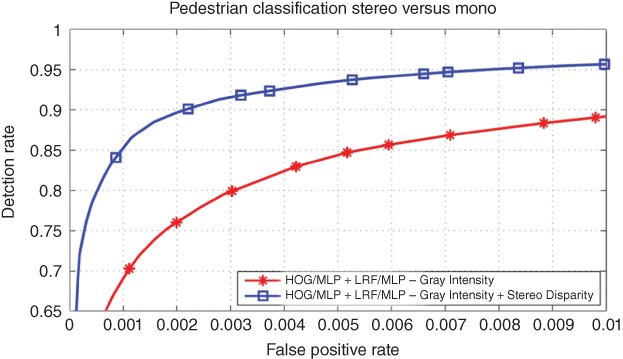
Figure 2.14 ROC curve illustrating the performance of a pedestrian classifier using intensity only (red) versus a classifier additionally exploiting depth (blue). The depth cue reduces the false-positive rate by a factor of five
The sketched system is highly efficient and powerful at the same time. However, the limited field of view of the used stereo system prohibits the recognition of pedestrians while turning at urban intersections. We used the wide-angled camera installed for traffic light recognition to check for pedestrians in those situations. Traffic light recognition was switched off and an unconstrained pedestrian search process was performed in those situations.
2.2.3.3 Vehicle Detection
For vision-based vehicle detection in the near range, a similar system concept as outlined earlier for pedestrian recognition including Stixel-based ROI generation can be used. However, the high relative velocities of approaching vehicles require a much larger operating range of the vehicle detection module than what is needed for pedestrian recognition. For Autonomous Driving in cities, it is desirable to detect and track oncoming vehicles at distances larger than 120m (equivalent to 4 seconds look ahead in city traffic) (see Figure 2.15). For highway applications, one aims at distances of 200m to complement active sensors over their entire measurement range.
Since one cannot apply stereo-based ROI generation for the long range, it has to be replaced by a fast monocular vehicle detector, that is, a Viola–Jones cascade detector (see Viola and Jones (2001b)). Since its main purpose is to create regions of interest for a subsequent strong classifier described earlier, one can easily tolerate the inferior detection performance of the Viola–Jones cascade framework compared to the state of the art and exploit its unrivaled speed.
Precise distance and velocity estimation of detected vehicles throughout the full distance range pose extreme demands on the accuracy of stereo matching as well as on camera calibration. In order to obtain optimal disparity estimates, one can perform an additional careful correlation analysis on the detected object. Pinggera et al. (2013) show that an EM-based multi-cue segmentation framework is able to give a sub-pixel accuracy of 0.1 px and allows precise tracking of vehicles 200m in front.

Figure 2.15 Full-range (0–200m) vehicle detection and tracking example in an urban scenario. Green bars indicate the detector confidence level
2.2.3.4 Traffic Light Recognition
Common Stereo Vision systems obey viewing angles within the range of ![]() –
–![]() . However, stopping at a European traffic light requires a viewing angle of up to
. However, stopping at a European traffic light requires a viewing angle of up to ![]() to see the relevant light signal right in front of the vehicle. At the same time, a comfortable reaction to red traffic lights on rural roads calls for a high image resolution. For example, in case of approaching a traffic light at 70km/h, the car should react at a distance of about 80m, which implies a first detection at about 100m distance. In this case, given a resolution of 20 px/
to see the relevant light signal right in front of the vehicle. At the same time, a comfortable reaction to red traffic lights on rural roads calls for a high image resolution. For example, in case of approaching a traffic light at 70km/h, the car should react at a distance of about 80m, which implies a first detection at about 100m distance. In this case, given a resolution of 20 px/![]() , the illuminated part of the traffic light is about
, the illuminated part of the traffic light is about ![]() px, which is the absolute minimum for classification. For practical reasons, a 4 MP color imager and a lens with a horizontal viewing angle of approximately
px, which is the absolute minimum for classification. For practical reasons, a 4 MP color imager and a lens with a horizontal viewing angle of approximately ![]() were chosen in the experiments presented here as a compromise between performance and computational burden.
were chosen in the experiments presented here as a compromise between performance and computational burden.
Traffic light recognition involves three main tasks: detection, classification, and selection of the relevant light at complex intersections. If the 3D positions of the traffic lights are stored in the map, the region of interest can easily be determined in order to guide the search. Although color information delivered by the sensor helps in this step, it is not sufficient to solve the problem reliably.
The detected regions of interest are cropped and classified by means of a Neural Network classifier. Each classified traffic light is then tracked over time to improve the reliability of the interpretation (see Lindner et al. (2004) for details).
In practice, the classification task turns out to be more complex than one might expect. About ![]() of the 155 traffic lights along the route from Mannheim to Pforzheim turned out to be hard to recognize. Some examples are shown in Figure 2.16. Red lights in particular are very challenging due to their low brightness. One reason for this bad visibility is the strong directional characteristic of the lights. Lights above the road are well visible at larger distances while they become invisible when getting closer. Even the lights on the right side, which one should concentrate on when getting closer, can become nearly invisible in case of a direct stop at a red light. In these cases, traffic light change detection monitoring the switching between red and green is more efficient than classification.
of the 155 traffic lights along the route from Mannheim to Pforzheim turned out to be hard to recognize. Some examples are shown in Figure 2.16. Red lights in particular are very challenging due to their low brightness. One reason for this bad visibility is the strong directional characteristic of the lights. Lights above the road are well visible at larger distances while they become invisible when getting closer. Even the lights on the right side, which one should concentrate on when getting closer, can become nearly invisible in case of a direct stop at a red light. In these cases, traffic light change detection monitoring the switching between red and green is more efficient than classification.

Figure 2.16 Examples of hard to recognize traffic lights. Note that these examples do not even represent the worst visibility conditions
2.2.3.5 Discussion
The recognition of geometrically well-behaved objects such as pedestrians or vehicles is a well-investigated topic (see Dollár et al. (2012), Gerónimo et al. (2010), and Sivaraman and Trivedi (2013)). Since most approaches rely on learning-based methods, system performance is largely dominated by two aspects: the training data set and the feature set used.
Regarding training data, an obvious conclusion is that performance scales with the amount of data available. Munder and Gavrila, for instance, have reported that classification errors are reduced by approximately a factor of two, whenever the training set size is doubled (see Munder and Gavrila (2006)). Similar beneficial effects arise from adding modalities other than gray-level imagery to the training set, for example, depth or motion information from dense stereo and dense optical flow (see Enzweiler and Gavrila (2011) and Walk et al. (2010)).
Given the same training data, the recognition quality significantly depends on the feature set used. For some years now, there has been a trend emerging that involves a steady shift from nonadaptive features such as Haar wavelets or HoGs toward learned features that are able to adapt to the data. This shift does not only result in better recognition performance in most cases, but it is also a necessity in order to be able to derive generic models that are not (hand-) tuned to a specific object class, but can represent multiple object classes with a single shared feature set. In this regard, deep convolutional neural networks (CNNs) represent one very promising line of research. The combination of such CNNs with huge data sets involving thousands of different object classes and lots of computational power has demonstrated outstanding multiclass recognition performance, for example, see Krizhevsky et al. (2012). Yet, much more research is necessary in order tofully understand all aspects of such complex neural network models and to realize their full potential.
A remaining problem with most object recognition approaches is that they are very restrictive from a geometric point of view. Objects are typically described using an axis-aligned bounding box of a constant aspect ratio. In sliding-window detectors, for example, the scene content is represented very concisely as a set of individually detected objects. However, the generalization to partial occlusion cases, object groups, or geometrically poorly-defined classes, such as road surfaces or buildings, is difficult. This generalization is an essential step to move from detecting objects in isolation toward gaining a self-contained understanding of the whole scene. Possible solutions to this problem usually involve a relaxation of geometric constraints and overall less object-centric representations, as will be outlined in the next section.
2.3 Challenges
Bertha's vision system was intensively tested off-line and during about 6500km of Autonomous Driving. The gained experience forced us to intensify our research on three topics, namely robustness, scene labeling, and intention recognition, in particular the intention of pedestrians.
2.3.1 Increasing Robustness
The built vision system delivers promising results in outdoor scenes, given sufficient light and good weather conditions. Unfortunately, they still suffer from adverse weather conditions. Similarly, the results deteriorate in low-light situations.
As mentioned in the discussion earlier, robustness can be improved if more information is included in the optimization process. As an example, we consider the disparity estimation task. When the windshield wiper is blocking the view (see Figure 2.17 left), stereo vision algorithms cannot correctly measure the disparity (see Figure 2.17 second from right). However, looking at the whole image sequence as opposed to only the current stereo pair, one can use previous stereo reconstructions and ego-motion information as a prior for the current stereo pair (see e.g., Gehrig et al. (2013)). This temporal stereo approach results in more stable and correct disparity maps. The improvement is exemplified in Figure 2.17 on the right. Since the temporal information just changes the data term of the SGM algorithm, the computational complexity does not increase much.
Similarly, more prior information can also be generated off-line by accurate statistics of typical disparity distributions from driver assistance scenarios. When using such simple information as a weak prior, one can already reduce the number offalse-positive Stixels (“phantom objects”) under rainy conditions by more than a factor of 2 while maintaining the detection rate (see Gehrig et al. (2014)).
Another option to increase robustness is confidence information. Most dense stereo algorithms deliver a disparity estimate for every pixel. Obviously, the confidence of this estimate may vary significantly from pixel to pixel. If a proper confidence measure that reflects how likely a measurement may be considered to be correct is available, this information can be exploited in subsequent processing steps. When using confidence information in the Stixel segmentation task, the false-positive rate can be reduced by a factor of six while maintaining almost the same detection rate (see Pfeiffer et al. (2013)).

Figure 2.17 Two consecutive frames of a stereo image sequence (left). The disparity result obtained from a single image pair is shown in the second column from the right. It shows strong disparity errors due to the wiper blocking parts of one image. The result from temporal stereo is visually free of errors (right) (see Gehrig et al. (2014))
2.3.2 Scene Labeling
A central challenge for Autonomous Driving is to capture relevant aspects of the surroundings and—even more important—reliably predict what is going to happen in the near future. For a detailed understanding of the environment, a multitude of different object classes needs to be distinguished. Objects of interest include traffic participants such as pedestrians, cyclists, and vehicles, as well as parts of the static infrastructure such as buildings, trees, beacons, fences, poles, and so on.
As already mentioned in the discussion, classical sliding window-based detectors do not scale up easily to many classes of varying size and shape, asking for novel generic methods that allow fast classification even for a large number of classes.
One way to approach the problem is scene labeling, where the task is to assign a class label to each pixel in the image. Recent progress in the field is driven by the use of super-pixels. Several of the current top-scoring methods encode and classify region proposals from bottom-up segmentations as opposed to small rectangular windows around each pixel in the image (see Russell et al. (2006)).
Furthermore, in terms of an integrated system architecture, it is “wise” to provide a generic medium-level representation of texture information, which is shared across all classes of interest, to avoid computational overhead. A suitable method for this is the bag-of-features approach, where local feature descriptors are extracted densely for each pixel in the image. Each descriptor is subsequently mapped to a previously learned representative by means of vector quantization, yielding a finite set of typical texture patterns. To encode an arbitrary region in the image, a histogram of the contained representatives is built, which can finally be classified to obtain the object class of the region.
Any super-pixel approach can provide the required proposal regions, while recent work shows that the Stixel representation is a well-suited basis for efficient scene labeling of outdoor traffic (see Scharwächter et al. (2013)). Proposal regions can be generated rapidly by grouping neighboring Stixels with similar depth.
Stereo information not only helps to provide good proposal regions but can also be used to improve classification. In addition to representative texture patterns, the distribution of typical depth patterns can be used as an additional channel of information yielding bag-of-depth features.
In Figure 2.18, a scene labeling result is shown together with the corresponding stereo matching result and the Stixel representation. Stixel-based region candidates are classified into one of five classes: ground plane, vehicle, pedestrian, building, and sky. Color encodes the detected class label. This example does not exploit the color information. However, if classes like “tree,” “grass,” or “water” are of interest, color plays an important role and can easily be added to the classification chain.

Figure 2.18 Scene labeling pipeline: input image (a), SGM stereo result (b), Stixel representation (d), and the scene labeling result (c)
2.3.3 Intention Recognition
Video-based pedestrian detection has seen significant progress over the last decade and recently culminated in the market introduction of active pedestrian systems that can perform automatic braking in case of dangerous traffic situations. However, systems currently employed in vehicles are rather conservative in their warning and control strategy, emphasizing the current pedestrian state (i.e., position and motion) rather than prediction to avoid false system activations. Moving toward Autonomous Driving, warnings will not suffice and emergency braking should still be the last option. Future situation assessment requires an exact prediction of the pedestrian's path, for example, to reduce speed when a pedestrian is crossing in front of the vehicle.
Pedestrian path prediction is a challenging problem due to the highly dynamic nature of their motion. Pedestrians can change their walking direction in an instant or start/stop walking abruptly. The systems presented until now only react to changes in pedestrian dynamics and are outperformed by humans (see Keller and Gavrila (2014)) who can anticipate changes in pedestrian behavior before they happen. As shown in Schmidt and Färber (2009), predictions by humans rely on more information than pedestrian dynamics only. Thus, humans are able to differentiate between a pedestrian that is aware of an approaching vehicle and one that is not and use this additional context information. As a consequence, humans are able to predict that a pedestrian aware of the vehicle will probably not continue on a collision course but rather stop or change walking speed. A system relying only on previously observed dynamics will predict that the pedestrian will continue to walk until it observes otherwise.
Future systems for pedestrian path prediction will need to anticipate changes in behavior before they happen and, thus, use context information, just like humans. For example, the motion of the pedestrian when approaching the curb is decisive. Work presented in Flohr et al. (2014) already goes in this direction by additionally estimating head and body orientations of pedestrians from a moving vehicle. Figure 2.19 shows that the resolution of imagers commercially used today is sufficient to determine the pose of the pedestrian. Further work will need to focus on integrating situational awareness (and other context information) into pedestrian path prediction.

Figure 2.19 Will the pedestrian cross? Head and body orientation of a pedestrian can be estimated from onboard cameras of a moving vehicle.  means motion to the left (body),
  is toward the camera (head)
2.4 Summary
When will the first Autonomous Vehicle be commercially available? Will it be capable of autonomous parking or Autonomous Driving on highways?
If you like to have a level 2 system, you can find them already on the market. If you think of a real level 3 system that allows you to forget the driving task on the highway for a while, there is no answer today. But at least three big questions: Can we guarantee that our car can manage every unexpected situation safely? How can we prove the reliability of the complete system if we have to guarantee an error rate of less than ![]() per hour? Can we realize such a system including highly sophisticated sensors and super-reliable fail-safe hardware for a reasonable price that people are willing to pay?
per hour? Can we realize such a system including highly sophisticated sensors and super-reliable fail-safe hardware for a reasonable price that people are willing to pay?
If we cannot answer all these questions positively at the present moment, we could think of alternative introduction strategies. If speed turns out to be the key problem, an automation of traffic jam driving might be a way out of the dilemma. Lower speeds limit the risk of serious hazards and would probably require less sensor redundancy such that the system could be made available at a lower price.
Nevertheless, I do not doubt that Autonomous Driving will become part of our lives in the foreseeable future. People are asking for this possibility as they want to use their time in the car for business and entertainment. Authorities are asking for this mode because they are hoping for fewer accidents. International regulations like the Vienna Convention on Road Traffic have recently been changed to allow Autonomous Driving.
While the DARPA Urban Challenge was dominated by laser scanners and radars, recent research shows that computer vision has matured and become indispensable for Scene Understanding. There is no other sensor that can be used to answer the multitude of questions arising in complex urban traffic. Modern stereo vision delivers precise and complete 3D data with high spatial resolution in real time. Super-pixels like Stixels allow for efficient globally optimal Scene Understanding. Thanks to progress in machine learning and increased computational power on FPGAs and graphical processing units, relevant objects can be detected fast and reliably.
However, there are still important aspects requiring further research.
- It is questionable whether precise localization and feature maps are really necessary for Autonomous Driving. It would be beneficial if a standard map was sufficient to plan the route and to extract all other information from the observed scene. Recent work in Zhang et al. (2013) raises hope that this can be achieved.
- In urban traffic, relevant objects are often partially occluded by other objects or traffic participants. Using the context might help to improve the performance and get closer to the excellence of human vision.
- The field of view of common stereo vision systems is sufficient for highway driving only. In cities we need multicamera systems or significantly higher resolution of automotive compliant imagers. The necessary computational power will become available, thanks to the ongoing progress in consumer electronics.
- An Autonomous Car must be able to stop in front of any obstacle that can cause serious harm. As this requirement limits its maximum speed, the early detection of small objects on the road requires particular attention.
During the last years, deep convolutional neural networks (DCNNs) have shown impressive results in classification benchmarks (see Krizhevsky et al. (2012)). Very recently, a new approach was presented in Szegedy et al. (2013), which does not only classify but also precisely localizes objects of various classes in images. The future will reveal whether these new techniques making use of the available big data will lead to a revolution of computer vision for autonomous vehicles.
Remember, just 25 years ago, researchers started putting cameras and huge computer systems into cars. None of them expected the progress that has been achieved in the meantime. This raises optimism that image understanding will get closer and closer to human visual perception in the future, allowing for Autonomous Driving not only on simply structured highways but also in complex urban environments.
Acknowledgments
The author thanks Markus Enzweiler, Stefan Gehrig, Henning Lategahn, Carsten Knöppel, David Pfeiffer, and Markus Schreiber for their contributions to this chapter.