Introduction
1. Jiawi Han and Micheline Kamber. (2006). Data mining: Concepts and techniques San Francisco: Elsevier.
Chapter 1
1. Damodaran Online. The data page. Retrieved August 15, 2010, from http://pages.stern.nyu.edu/∼adamodar/New_Home_Page/data.html as part of a larger data set.
2. U.S. Office of Personnel Management. Federal Civilian Workforce Statistics: The Fact Book, 2007 Edition. Retrieved from http://www.opm.gov/feddata/factbook/2007/2007FACTBOOK.pdf
3. American Public Transportation Association. 2010 Public Transportation Fact Book, 61st ed. April 2010. Retrieved from http://www.apta.com/resources/statistics/Documents/FactBook/APTA_2010_Fact_Book.pdf
4. Unlinked passenger trips refers to the total number of passengers who board public transit vehicles. Each passenger is counted each time that person boards a vehicle even though the boarding may be the result of a transfer from another route while on the same journey. Thus unlinked passenger trips will be larger than actual ridership.
5. Outlier does not necessarily mean mistake or error. Here, the data for New York City is absolutely correct; it is just well outside the range of any other observation.
6. The actual calculation for this specific data set is –0.042, which is extremely close to zero. The exact value would depend on the number of observations included, but it would always be close to zero.
7. The assignment of Age as X and Tag Number as Y is completely arbitrary and for correlation does not matter. The resulting value for the correlation coefficient would be exactly the same if Age were assigned as Y and Tag Number were assigned as X. The proof of this is left to interested readers.
8. SPSS stands for Statistical Program for the Social Sciences, but everyone just calls it SPSS.
9. It actually does not hurt anything to include the cells with the column labels (e.g., “=CORREL(A1:A8,B1:B8)”), as they are just ignored by Excel.
10. The “bi-” in “bivariate” comes from the Latin bis, meaning “twice” and bini, meaning “in twos.”
11. It is helpful if the reader has a general knowledge of hypothesis testing on means and proportions as well as the Student t-distribution. However, students without familiarity with these topics should be able to read and comprehend most of this section.
Chapter 2
1. With simple regression, it is not uncommon to leave out the first subscript of the Xs; that is, write X1,1 as X1, X1,2 as X2, and so on. If you do this, you must be careful as it can lead to confusion in multiple regression.
2. There is a second set of equations that can be used to calculate simple regression coefficients. Normally, we would avoid giving two equations that accomplish exactly the same thing. However, you may run into this set of equations in other courses—such as operation management or forecasting—so they are presented here for completeness:
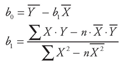
This set of equations gives the same results and they have no computational advantage.
3. ANOVA is short for analysis of variance.
4. This statement assumes α = 0.05, as it usually does in business statistics.
Chapter 3
1. The term is the combination of homo, from the Latin homos meaning one and the same or similar, and the Greek skedastokos, meaning able to disperse. Thus the term refers to having equal or the same variances.
2. The assumption of normally distributed error terms uncorrelated with one another automatically implies the independence of the error terms.
3. Interested students may wish to repeat our analysis using any or all of the counts for bronze, silver, or gold as the dependent variable to see how they compare with the results presented here.
4. The value of this coefficient is actually 4.69047952958057 × 10–09 or 0.000000000469047952958057. It is this low not because the variable is unimportant but rather because the units used to measure income (dollars) are so large relative to the units used to measure rank. As a general rule, you cannot gauge the importance of a variable by the magnitude of its coefficient.
5. Again, the value is small due to the units used to measure Web Hits.
6. Recall from the last chapter that correlation is only defined between pairs of variables.
7. In all these calculations, results are rounded for display but have been carried out in all the calculations.
8. Once any two of SSR, SSE, and SST are computed, you can always find the third using this formula.
9. Highlight the cells containing the formulas, right-click with the mouse, and select Copy. With the formulas still highlighted, right-click again and under the Paste options will be an icon of a clipboard with a 123 in the bottom right corner. Select this Paste option. This replaces the formulas with their current value.
10. As we will see later, in special cases, the overall model can be significant even when none of the independent variables is significant or at least when they are all included in the model.
11. “Auto” comes from the Greek autos, meaning same or self. Thus autocorrelation refers to correlation with oneself. In this case, the error terms are being correlated with themselves; more specifically, the correlation between pairs of error terms is taken at a constant interval.
12. The calculations are not exactly this straightforward. Rejecting 10 true null hypotheses (200 × 0.05) due to sampling error alone requires that all 200 null hypotheses be true—that is, that all 200 variables be insignificant. If most of the variables were truly significant as they were in this case, then the number of rejections of true null hypotheses would be correspondingly low because rather than having (200 × 0.05) we would have a number much smaller than 200 in this calculation.
13. Because of the way Excel handles p-values, you must divide the p-value by 2 for a one-tailed test.
Chapter 4
1. Most statistical packages support all or most of these. It is up to the operator to select the actual procedure to be used.
2. Because r2 always goes up when you add variables, it will always go down when you drop a variable. However, when dropping an insignificant variable, this drop is often slight and may be hard to pick up if you normally format r2 to four or five decimal points.
3. The values of one and zero make the math easier to understand and the model easier and are traditionally used, but any two numbers could be used and would have the same overall effect.
4. Again, this simply makes understanding the model easier. We could as easily code the data the other way—that is, zero for when the event happened and one when it did not happen.
5. Or planes when there are two nondummy independent variable, or hyperplanes when there are three or more nondummy independent variables.
6. http://www.presidentialelection.com/follow_the_money/ accessed on April 9, 2011.
7. For the interested reader, this was accomplished using an advanced statistical procedure called factor analysis. The operation of factor analysis is beyond the scope of this textbook. Additionally, factor analysis cannot be performed using Excel. The author created this data set using SPSS. Interested readers are referred to an advanced statistical reference book, such as Bobko (1995), Correlation and Regression: Principles and Applications for Industrial/Organizational Psychology and Management. New York: McGraw-Hill.
8. Of course, this can also be caused by a bad sample.
9. For a two-tailed test, we double the alpha value shown in the table, and the ranges 0 – dL and 4-dL – 4 simply become rejection regions.
10. Refer to an advanced statistics textbook for Durbin-Watson tables.
11. In finance, this raw form is called nominal dollars.
12. Recall from earlier that part of this term comes from the Greek skedastokos, meaning able to disperse. The hetero comes from the Latin heteros, meaning other than usual, other, or different.