CHAPTER 3

Multiple Regression

In the last chapter, we saw how to construct a simple regression model. Simple regression described the linear relationship between one dependent variable and a single independent variable. However, in most business situations it takes more than a single independent variable to explain the behavior of the dependent variable. For example, a model to explain company sales might need to include advertising levels, prices, competitor actions, and perhaps many more factors. This example of using various independent variables—like advertising, price, and others—is a good mental model to use when thinking about multiple regression.

When we wish to use more than one independent variable in our regression model, it is called multiple regression. Multiple regression can handle as many independent variables as is called for by your theory—at least as long as you have an adequate sample size. However, like simple regression, it, too, is limited to one dependent, or explained, variable.

As we will see, multiple regression is nothing more than simple regression with more independent variables. Most business situations are complex enough that using more than one independent variable does a much better job of either describing how the independent variables impact the dependent variable or producing a forecast of the future behavior of the dependent variable.

Multiple Regression as Several Simple Regression Runs

In addition to the name change, the procedure for calculating the regression model itself changes, although that is not immediately obvious when performing those calculations using Excel. Before we get into that, we will illustrate multiple regression using simple regression.

Simple Regression Example

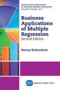
Figure 3.1 shows machine maintenance data for 20 machines in a medium-sized factory. The first column shows the number of hours between its last breakdowns, the second column shows the age of the machine in years, and the third column shows the number of operators. Because we have not yet seen how to use more than one independent variable in regression, we will perform simple regression with breakdown hours as the dependent variable and age as the independent variable. The results of that simple regression are shown in Figure 3.2.

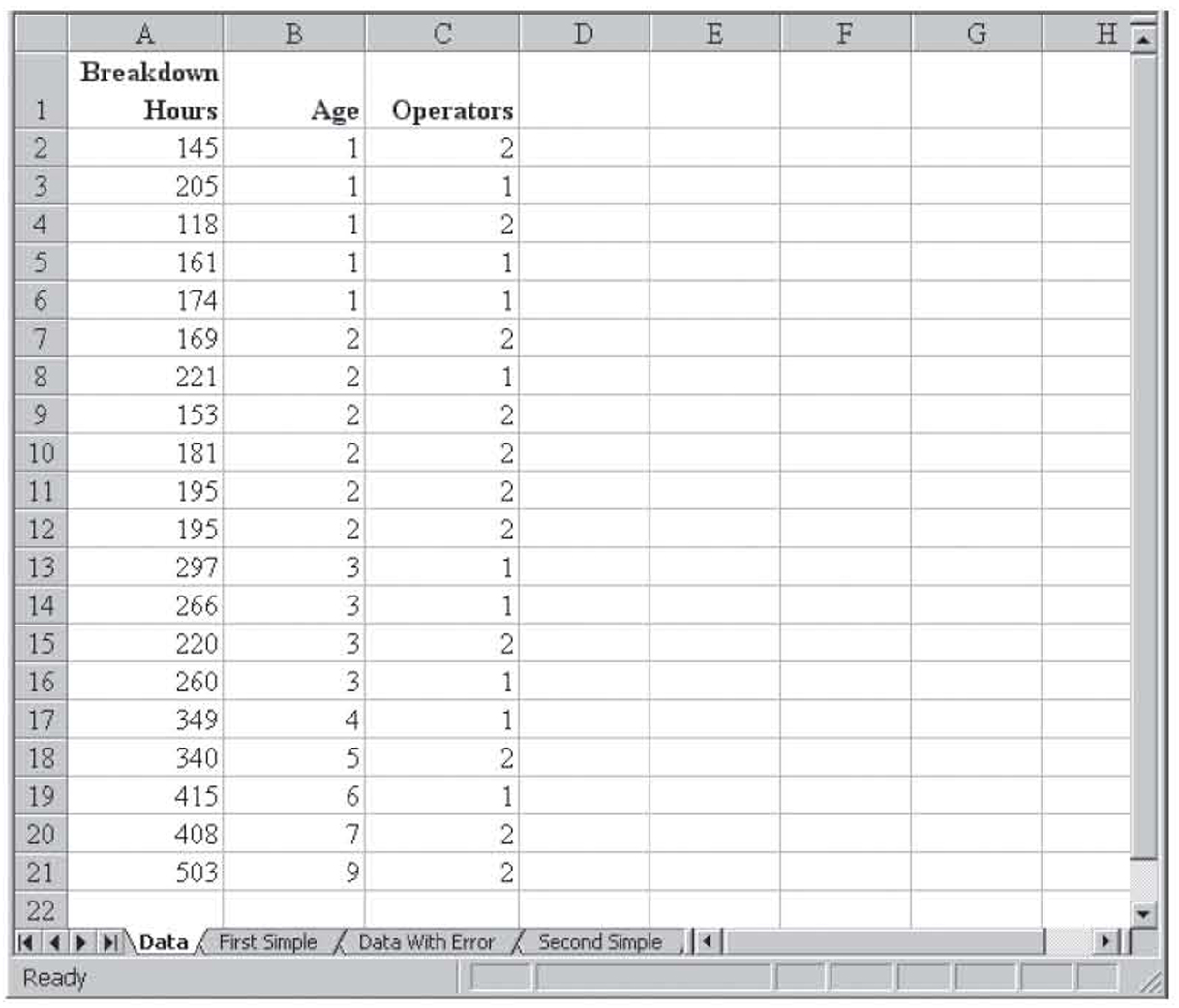
Figure 3.1 An Excel worksheet with one dependent variable and two independent variables

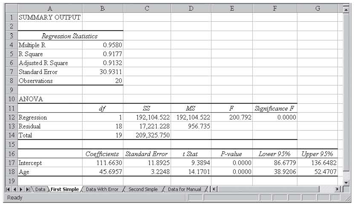
Figure 3.2 Using simple regression and one of the two independent variables

As you can see from Figure 3.2, the overall model is significant and the variation in the age of the machine explains almost 92 percent (0.9177) of the variation in the breakdown hours, giving the resulting regression equation:

The Resulting Regression Equation

Breakdown Hours = 111.6630 + 45.6957(Age)

As good as these results are, perhaps the addition of the number of operators as a variable can improve it. In order to see this, we will begin by computing the breakdown hours suggested by the model by plugging the age of the machine into the previous equation. We will then subtract this value from the actual value to obtain the error term for each machine. Those results are shown in Figure 3.3.

Figure 3.3 Calculating the part of the breakdown hours not explained by the age of the machine

Notice that the sum of the error terms is zero. This is a result of how regression works and will always be the case. The error values represent the portion of the variation in breakdown hours that are unexplained by age, because, if age was a perfect explanation, all the error values would be zero. Some of this variation is, naturally, random variation that is unexplainable. However, some of it might be due to the number of operators because that varies among the machines. A good reason for calling this a residual, rather than error, is that parts of this error might, in fact, be explained by another variable—the number of operators in this case.

We can check by performing a second simple regression, this time with residual as the dependent variable and number of operators as the independent variable. Those results are shown in Figure 3.4.

Figure 3.4 Performing simple regression between the residual and the number of operators

Notice that this regression is also significant. The variable for the number of operators explains 71 percent (0.7119) of the variation in the residual term or 71 percent of the remaining 8 percent unexplained variation of the original simple regression model, giving the resulting equation:

Resulting Regression Equation

Residual = 77.1358 – 49.7650(Age)

Although this approach of using multiple simple regression runs seems to have worked well in this simplified example, we will see a better approach in the next section. Additionally, with more complex regression applications with many more variables, this approach would quickly become unworkable.

Multiple Regression

In the previous example, we performed simple regression twice: once on the dependent variable and the first independent variable and then on the leftover variation and the second independent variable. With multiple regression, we simultaneously regress all the independent variables against a single dependent variable. Stated another way, the population regression model for a single dependent variable Y and a set of k independent variables X₁, X₂, . . . , X_k gives the following:

Population Regression Model

Y = β₀ + β₁X₁ + β₂X₂ + … + β_kX_k + ε

where β₀ is the Y-intercept, each of the β_i’s for i = 1 to k is the slope of the regression surface with respect to the variable X_i, and e is the error term. This error term is also commonly referred to as the residual.

Of course, we rarely work with population data, so we are usually interested in calculating the sample regression model as an estimate of the population regression model:

Sample Regression Model

Y = b₀ + b₁X₁ + b₂X₂ + … + b_kX_k + ε

where b_i is the sample statistic that estimates the population parameter β_i.

As you may recall from the last chapter, the graph of the results of simple regression is a line. That is because there are two variables, one independent variable and one dependent variable. With only two variables, the data are defined in two-dimensional space and thus a line. With multiple regression, we have at least three dimensions and possibly many more. When there are two independent variables and one dependent variable, we have three-dimensional space and the results of the regression are a plane in this space. When we exceed two independent variables, we exceed three-dimensional space and, therefore, we exceed our ability to graph the results as well as our ability to visualize those results. When this happens, the results of the regression are said to be a hyperplane that exists in hyperspace.

Assumptions for Multiple Regression

As you would expect, the assumptions for multiple regression are very similar to the assumptions for simple regression:

   1.  For any specific value of any of the independent variables, the values of the dependent variable Y are normally distributed. This is called the assumption of normality. As a result of the dependent variable being normally distributed, the error terms will also be normally distributed.

   2.  The variance for the normal distribution of possible values for the dependent variable is the same for each value of each independent variable. This is called the equal variance assumption and is sometimes referred to as homoscedasticity.¹

   3.  There is a linear relationship between the dependent variable and each of the independent variables. This is called the linearity assumption. Because the technique of regression (simple or multiple) only works on linear relationships, when this assumption is violated, that independent variable is usually found to be insignificant. That is, it is found not to make any important contribution to the model. As a result, this assumption is self-enforcing.

   4.  None of the independent variables are correlated with each other. Although this assumption does not have a name, we will refer to its violation as multicollinearity in a later section, so we will refer to this assumption as the nonmulticollinearity assumption.

   5.  The observations of the dependent variable are independent of each other. That is, there is no correlation between successive error terms, they do not move around together, and there is no trend.² This is naturally called the independence assumption. In a later section, we will refer to the violation of this assumption as autocorrelation.

 

Using Excel to Perform Multiple Regression

Excel is able to perform the multiple regression calculations for us. The steps are the same as with simple regression. You begin by clicking on the Data tab, then Data Analysis, and then selecting Regression from the list of techniques. Excel makes no distinction between simple and multiple regression. Fill in the resulting dialog box just as before, only this time enter the two columns that contain the two independent variables. This is shown in Figure 3.5.

Figure 3.5 Performing multiple regression with Excel

The steps for running multiple regression in Excel are the exact same steps we performed to run simple regression in Excel. In fact, making a distinction between simple and multiple regression is somewhat artificial. As it turns out, some of the complexities that occur when you have two or more independent variables are avoided when there is only one independent variable, so it makes sense to discuss this simpler form first. Nevertheless, both simple and multiple regression are really just regression.

One note is critical regarding the way Excel handles independent variables. Excel requires that all the independent variables be located in contiguous columns. That is, there can be nothing in between any of the independent variables, not even hidden columns. This is true regardless of whether you have just two independent variables or if you have dozens. (Of course, this is not an issue in simple regression.) It also requires that all the observations be side by side. That is, all of observation 1 must be on the same row, all of observation 2 must be on the same row, and so on. It is not, however, required that the single dependent variable be beside the independent variables or that the dependent variable observations be on the same rows as their counterparts in the set of independent variables. From a data management perspective, this is nevertheless a very good idea, and this is the way that we will present all the data sets used as examples.

Additionally, Excel’s regression procedure sometimes becomes confused by merged cells, even when those merged cells are not within the data set or its labels. If you get an error message saying Excel cannot complete the regression, the first thing you should check for is merged cells.

Example

Figure 3.6 shows the results of running multiple regression on the machine data we have been discussing. Notice that the results match the appearance of the simple regression results with the exception of having one additional row of information at the bottom to support the additional independent variable. This is, of course, to be expected.

Figure 3.6 The result of running multiple regression on the machine data discussed earlier in this chapter

In the machine example, we had the first, simple regression equation:

First Simple Regression Equation

Ŷ = 111.6630 + 45.6957X

and the second regression equation was

Second Regression Equation

Ŷ = 77.1358 – 9.7650b₂

Adding these together, we obtain the following equation:

Combined Regression Equation

Ŷ = 183.7988 + 45.6957b₁ – 49.7650b₂

Note that this is similar to, but not exactly equal to, the multiple regression equation we just obtained:

Multiple Regression Equation

Ŷ = 185.3875 + 47.3511b₁ – 50.7684b₂

One of the assumptions of multiple regression is the nonmulticollinearity assumption: There is no correlation between the independent variables. In this example, there is slight (0.1406) correlation between the two independent variables. It is this slight correlation that prevents the total of the individual simple regression equations from totaling to the multiple regression equation. The higher the correlation, the greater the difference there will be between the equations derived using these two approaches. Because there is virtually always some degree of correlation between independent variables, in practice we would never approach a multiple regression equation as a series of simple regression equations.

Another Example

Oftentimes, businesses have a lot of data but their data are not in the right format for statistical analysis. In fact, this so-called dirty data is one of the leading problems that businesses face when trying to analyze the data they have collected. We will explore this problem with an example.

Figure 3.7 shows the medal count by country for the 2000 Olympic Games in Sydney, Australia. It shows the number of gold, silver, and bronze medals along with the total medal count. Also shown are the population and per capita gross national product (GNP) for each country. We will use this information for another multiple regression example, but we must address the dirty data first.

Figure 3.7 Data from the 2000 Olympic Games in Sydney, Australia

 

Data Cleaning

Before we continue with the multiple regression portion of this example, we will take this opportunity to discuss data cleaning. Data cleaning is when we resolve any problems with the data that keep us from using it for statistical analysis. These problems must be resolved before these data can be used for regression, or anything else for that matter. Otherwise, any results you obtain will not be meaningful.

When this Sydney Olympics data set was first put together, it had a couple of significant problems. The first problem is that population size and GNP were not available for all the countries. For example, an estimate of GNP was not available for Cuba. The number of countries for which a full set of data was not available was very small, and their medal count was minor so these countries were dropped from the data set.

The second problem was that the per capita GNP was naturally measured in their own currency and a standard scale was needed because it makes sense to use a standard to compare values of a variable where each observation was measured using a different scale. This was handled by converting all the currencies to U.S. dollars, but this raised a third problem: Because the value of currencies constantly fluctuates against the U.S. dollar, which conversion value should be used? We decided to use the conversion value in effect around the time of the Olympics, and the data shown is based on that conversion.

It is not uncommon for business data to require cleaning before being ready for use in statistical analysis. In this context, we use statistical analysis in a very broad sense and not just in reference to multiple regression. As long as only a few data points are discarded and as long as any data conversions are reasonable, the data cleaning should not have too much of an impact on the results of any statistical analysis performed on the data. In any case, we do not have much of a choice. Without cleaning, the data would not be in a useable form.

Olympics Example Continued

Returning to our data set from the 2000 Sydney Olympics, we will use total medal count³ as the dependent variable and per capita GNP and population as the independent variables. Figure 3.8 shows the dialog box filled out to perform the multiple regression and Figure 3.9 shows the results.

Figure 3.8 The dialog box used to perform multiple regression on the 2000 Olympic Games data set

Figure 3.9 The results of the multiple regression analysis on the 2000 Olympic Games data set

 

r² Can Be Low but Significant

Notice that in the Sydney Olympics example the variations in population and per capita GNP explain only 21 percent (0.2104) of the variation in total medals, yet the overall model is significant and the individual variables are all significant as well. This is an important point. It is not necessary for r² to be high in order for the overall model to be significant. This is especially true with larger data sets—that is, with higher numbers of observations. When businesses analyze massive data sets, it is not uncommon for even unrelated variables to show significant correlations for this very reason.

Students sometimes also make the mistake of thinking that only models with high r² values are useful. It is easy to see why students might believe this. Because r² represents the percentage of the variation in the dependent variable that is explained by variation in the independent variables, one might conclude that a model that explains only a small percentage of the variation is not all that useful.

In a business situation, this is, in fact, a reasonable assumption. A forecasting model that explained only 21 percent of the variation in demand would not be very useful in helping to plan production. Likewise, a market analysis that ends up explaining only 21 percent of the variation in demand would likely have missed the more important explainer variables.

However, in other areas, explaining even a small percentage of the variation might be useful. For example, doctors might find a model that explained only 21 percent of the variation in the onset of Alzheimer’s disease to be very useful. Thus the decision about how useful a model is, at least once it has been found to be statistically significant, should be theory based and not statistically based. This requires knowledge of the field under study rather than statistics. This is the main reason that statisticians usually need help from knowledgeable outsiders when developing models.

Example

We will now look at an example involving celebrities. Although this is clearly a nonbusiness example (unless, of course, you are in the business of making movies), the procedures and considerations are exactly the same as performing a marketing analysis to try to understand why your product is (or is not) popular.

Forbes collected the following information on the top 100 celebrities for 2000:

    •  Earnings rank, or simply a rank ordering of 1999 earnings

    •  Earnings for 1999

    •  Web hits across the Internet

    •  Press clips from Lexis-Nexis

    •  Magazine covers

    •  Number of mentions on radio and television

The data are collected in the worksheet Celebrities.xls, which is shown in Figure 3.10. Forbes used this information to decide on a “power rank” for each celebrity. We will use multiple regression to try to discover the rationale behind the power rank. That regression is shown in Figure 3.11.

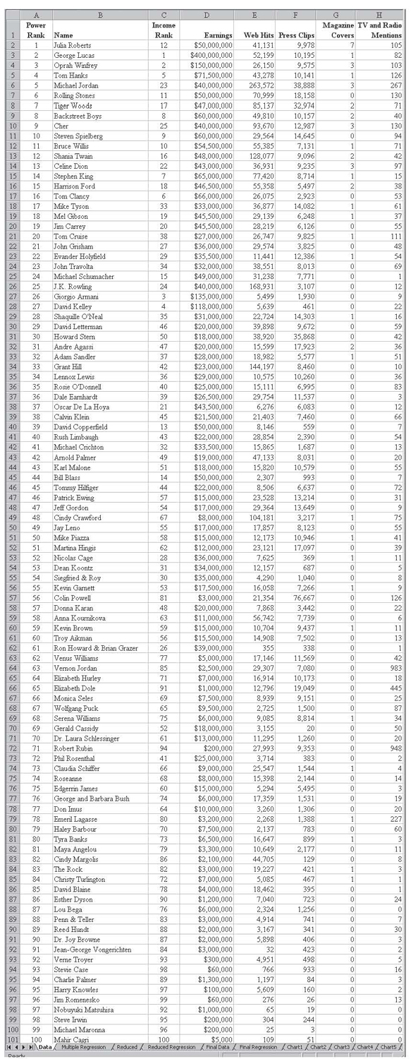
Figure 3.10 Forbes 2000 data on 100 celebrities

Figure 3.11 The multiple regression results on the year 2000 Forbes data on 100 celebrities with Power Rank as the dependent variable

The r² value is 0.9245, so over 92 percent of the variation in the power rank is explained by this data, giving the resulting equation:

Power Rank Equation

Power Rank = 17.2959 + 0.8270(Income Rank) + 0.00004⁴(Earnings) – 0.0001⁵(Web Hits) – 0.0005(Press Clips) – 2.4321(Magazine Covers) – 0.0220(TV and Radio Mentions)

Some of the signs in this equation seem unusual. We will have more to say about this later. But before we get into this, we need to discuss how to evaluate the significance of the overall model, as well as the significances of the individual components.

The F-Test on a Multiple Regression Model

The first statistical test we need to perform is to test and see if the overall multiple regression model is significant. After all, if the overall model is insignificant then there is no point is looking to see what parts of the model might be significant. Back with simple regression, we performed the following test on the correlation coefficient between the single dependent variable and the single independent variable and said that if the correlation was significant then the overall model would also be significant:

H₀ : ρ = 0

H₁ : ρ ≠ 0

With multiple regression, we can no longer use that approach. The reason is simple: If there are six independent variables, then there are six different correlations between the single dependent variable and each of the independent variables.⁶

With simple regression, a significant correlation between the single dependent and the single dependent variable indicated a significant model. With multiple regression, we may end up with data where some of the independent variables are significant whereas others are insignificant. For this reason, we need a test that will test all the independent variables at once. That is, we want to test the following:

H₀ : β₁ = β₂ =    = β_k = 0

H₁ : β_i ≠ for some i

In other words, we are testing to see that at least one β_i is not equal to zero.

Think about the logic for a minute. If all the β_i’s in the model equal zero, then the data we have collected is of no value in explaining the dependent variable. So, basically, in specifying this null hypothesis we are saying that the model is useless. On the other hand, if at least one of the β_i’s is not zero, then at least some part of the model helps us explain the dependent variable. This is the logic behind the alternative hypothesis. Of course, we will still need to delve into the model and figure out which part is really helping us. That is a topic for a later section.

We will use analysis of variance (ANOVA) to perform the test on the hypotheses shown previously. Before looking at the hypothesis test, a couple of notes are in order regarding the aforementioned hypotheses. First, notice that the null hypothesis does not specify the intercept, β₀. As with simple regression, we are rarely interested in the significance of the intercept. As discussed previously, it is possible that some of the β_i’s will be significant whereas others will be insignificant. As long as any one of them is significant, the model will pass the ANOVA test.

We will briefly review ANOVA as it relates to multiple regression hypothesis testing. Interested students should refer to a statistics textbook for more details. Figure 3.12 shows just the ANOVA section from the 2000 Sydney Olympics results regression shown previously. In this discussion, the numbers with arrows after them are shown in the figure as references to the items under discussion. They are not, of course, normally a part of the ANOVA results.

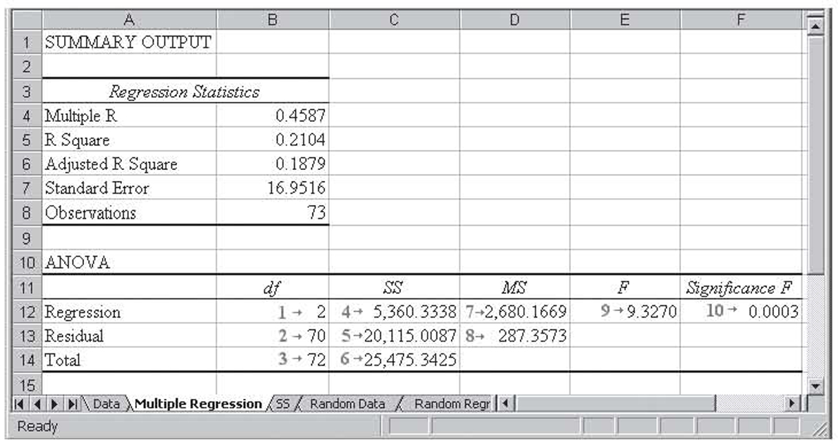
Figure 3.12 ANOVA section for the 2000 Sydney Olympics results regression

We will now discuss each of the notes shown in Figure 3.12.

   1.  The regression degrees of freedom is k, the number of independent variables (two in this case).

   2.  The residual (or error) degrees of freedom is n – k–1, or 73 – 2 – 1 = 70 in this case.

   3.  The total degrees of freedom is n –1, or 72 in this case.

   4.  This is the sums of squares (SS) regression. We will abbreviate this as SSR. Its calculation will be discussed in more detail shortly.

   5.  This is SS residual. In order to avoid confusion with SS regression, we will abbreviate this as SSE. Its calculation will be discussed in more detail shortly.

   6.  This is SS total. We will abbreviate this as SST. Its calculation will be discussed in more detail shortly.

   7.  This is mean square regression, or MS regression. We will abbreviate this as MSR. It is calculated as SSR / k.

   8.  This is mean square residual/error or MS residual. We will abbreviate this as MSE. It is calculated as SSE / (n – k – 1).

   9.  The F ratio is calculated as MSR/MSE. This value is chi square distributed with k,n – k – 1 degrees of freedom.

 10.  This is the p-value for the F-test. When it is less than 0.05, the overall model is significant, and when it is greater than 0.05, the overall model is not significant. That is, you reject the null hypothesis that all the β_k coefficients are zero. If the overall model is not significant, that is, if all the β_k coefficients are equal to zero, then there is no point in continuing with the regression analysis.

We will briefly review the calculation of SSR, SSE, and SST. However, because Excel and every other multiple regression program report these values, no additional emphasis will be placed on their manual calculation. Figure 3.13 shows the data from the 2000 Sydney Olympics with the information required to calculate all three sums of squares values. Note that some of the rows are hidden in this figure. That was done to reduce the size of the figure.

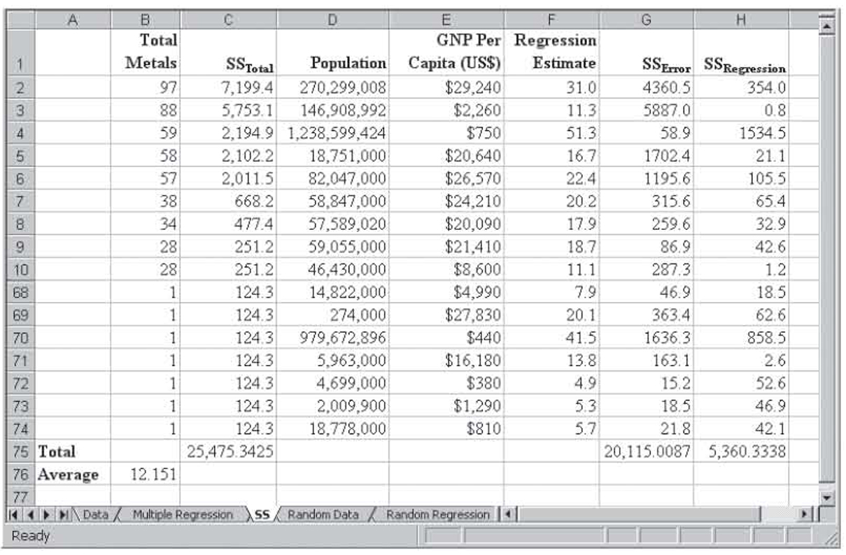
Figure 3.13 The values from the data from the 2000 Sydney Olympics that will be used to calculate the sums of squares values

From the data, the average of the number of medals won (Y) is 12.151, giving the following equation for SST:

SST

SST = Σ (Y – Y)²

For row 1, 97 – 12.151 = 84.8 and 84.8² = 7,199.4.⁷ For row 2, 88 – 12.151 = 75.8 and 75.8² = 5,753.1. These calculations are carried out for each of the data points, and the total of these squared values is 25,475.3425. This is the SST value shown back in Figure 3.12.

The formula for SSE is the following:

SSE

SSE = Σ (Y – Ŷ)²

For row 1, the predicted Y value is 31.0 and (97 – 31.0)² = 4,360.5. For row 2, the predicted Y value is 11.3 and (88 – 11.3)² = 5,887.0. These calculations are carried out for all the data, and the total of these squared values is 20,115.0087. This is the SSE value shown back in Figure 3.12.

At this point, there is no need to compute SSR because the formula

SST

SSR + SSE = SST

allows us to compute it based on SST and SSE.⁸ Nevertheless, SSR is represented by the following equation:

SSR

SSR = Σ (Ŷ – Y)²

For row 1, that gives us 31.0 – 12.151 = 18.8 and 18.8² = 354.0. For row 2, 11.3 – 12.151 = –0.9 and –0.9² = 0.8. These calculations are carried out for all the data, and the total of these squared values is 5,360.3338. This is the SSE value shown back in Figure 3.12.

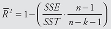
How Good Is the Fit?

In the last chapter on simple regression, we saw that r² represents the percentage of the variation in the dependent variable that is explained by variations in the independent variable. That relationship holds in multiple regression, only now more than one independent variable is varying. In the last chapter, we simply accepted this definition of r². Now that we have discussed ANOVA, we are ready to see how r² is calculated:

Calculation of r²

From this calculation and Figure 3.12, we have SSR = 5,360.3338 and SST = 25,475.3425. That gives us 5,360.3338/25,475.3425 = 0.2104. This is exactly the value shown in Figure 3.12 for r².

Notice that the numerator of this formula for r² is the variation explained by regression and the denominator is the total variation. Thus this formula is the ratio of explained variation to total variation. In other words, it calculates the percentage of explained variation to total variation.

The value of r² suffers from a problem when variables are added. We will illustrate this problem with an example.

Example

Figure 3.14 shows the data from the 2000 Sydney Olympics with four variables added. Each of these variables was added by using the Excel random number generator. These random numbers were then converted from a formula (=RAND()) to a hardwired number⁹ so their value would not change while the regression was being calculated and so you could experiment with the same set of random numbers. Although the numbers are still random, they can just no longer vary. Because these numbers were randomly generated, they should not help to explain the results at all. That is, they have absolutely no relationship to the number of medals won. As a result, you would expect that the percentage of variation explained (r²) would also not change.

Figure 3.14 The data for the 2000 Sydney Olympics with four completely random variables added

Figure 3.15 shows the results of the new multiple regression including the four random variables. As expected, none of these variables is significant. However, the r² value goes up from 0.2104 when the regression was run without the random variables to 0.2731 when the random variables are included. Why?

Figure 3.15 The results of running multiple regression on the 2000 Sydney Olympics data with four completely random variables added

With simple regression, the model is a line. A line is uniquely defined by two points, so simple regression on two points will always perfectly define a line. This is called a sample-specific solution. That is, r² will always be 1.00 even if the two variables have nothing to do with each other. For any regression with k independent variables, a model with k + 1 observations will be uniquely defined with r² of 1.00. Additionally, as the number of variables increases, even when those variables have no useful information, the value of r² will always increase. That is why r² increased in the previous example when the four random, and useless, variables were added. If we were to add more variables containing purely random data, r² would go up again. The opposite is also true. If you drop a variable from a model, even a variable like these random numbers that have no relationship to the dependent variable, r² will go down.

To account for r² increasing every time a new variable is added, an alternative measure of fit, called the adjusted multiple coefficient of determination, or adjusted r², is also computed using the following formula:

Multiple Coefficient of Determination, or Adjusted r²

As with r², the symbol R² is for the population value and r² is for the sample. Because this symbol is not used in computer printouts, we will just use adjusted r². Although r² always increases when another variable is added, the adjusted r² does not always increase because it takes into account changes in the degrees of freedom. However, the adjusted r² may also increase when unrelated variables are added, as it did in the previous example, increasing from 0.1879 to 0.2070. When the adjusted r² does increase with the addition of unrelated variables, its level of increase will generally be much less than r², as was the case here.

In certain rare cases, it is possible for the adjusted r² to be negative. The reason for this is explained in the sidebar in more detail, but it happens only when there is little or no relationship between the dependent variable and the independent variables.

Figure 3.16 Random data

Figure 3.17 The results of running multiple regression on the random data

Testing the Significance of the Individual Variables in the Model

So far, we have discussed our regression models in general terms, and we have only been concerned with whether the overall model is significant—that is, if it passes the F-test. As was discussed previously, passing the F-test only tells us that the overall model is significant, and if there are collinear variables, then one of the variables is significant, though not that all of them are significant. In other words, once one of these collinear variables is dropped out, at least one variable will be significant. We now need to explore how to test the individual b_i coefficients.

This test was not required with simple regression because there was only one independent variable, so if the overall model was significant, that one independent variable must be significant. However, multiple regression has two or more independent variables and the overall model will be significant if only one of them is significant.¹⁰ Because we only want significant variables in our final model, we need a way to identify insignificant variables so they can be discarded from the model.

The test of significance will need to be carried out for each independent variable using the following hypotheses:

H₀ : β_k = 0

H₁ : β_k ≠ 0

Of course, when there is reason to believe that the coefficient should behave in a predetermined fashion, a one-tailed test can be used rather than a two-tailed test. As always, the selection of a one-tailed or two-tailed test is theory based. Before discussing how to perform this hypothesis test on the slope coefficient for each variable, we need to discuss several problems with the test.

Interdependence

All the regression slope estimates come from a common data set. For this reason, the estimates of the individual slope coefficients are interdependent. Each individual test is then carried out at a common alpha value, say α = 0.05. However, due to interdependence, the overall alpha value for the individual tests, as a set, cannot be determined.

Multicollinearity

In multiple regression, we want—in fact we need—each independent variable to have a strong and significant correlation with the dependent variable. However, one of the assumptions of multiple regression is that the independent variables are not correlated with each other. When this assumption is violated, the condition is called multicollinearity. Multicollinearity will be discussed in more detail later. For now, it is enough to know that the presence of multicollinearity causes the independent variables to rob one another of their explanatory ability. When a significant variable has its explanatory ability reduced by another variable, it may test as insignificant even though it may well have significant explanatory abilities and even if it is an important variable from a theoretical perspective.

Autocorrelation

One of the assumptions of multiple regression is that the error or residual terms are not correlated with themselves. When this assumption is violated, the condition is called autocorrelation.¹¹ Autocorrelation can only occur when the data are time-series data—that is, measurements of the same variables at varying points in time. More will be said about autocorrelation later. For now, autocorrelation causes some variables to appear to be more significant than they really are, raising the chance of rejecting the null hypothesis.

Repeated-Measures Test

The problem of repeated measures is only a major concern when a large number of variables need to be tested. Alpha represents the percentage of times that a true null hypothesis (that the variable is insignificant when used with regression) will be rejected just due to sampling error. At α = 0.05, we have a 5 percent chance of rejecting a true null hypothesis (β_k = 0) just due to sampling error. When there are only a few variables, we need not be overly concerned, but it is not uncommon for regression models to have a large number of variables. The author constructed a regression model for his dissertation with over 200 variables. At α = 0.05, on average, this model could be expected to reject as many as 10 true null hypotheses just due to sampling error.¹²

Recall the following hypotheses:

H₀ : β_k = 0

H₁ : β_k ≠ 0

However, a one-tailed test could be performed if desired. The test statistic is distributed according to the Student t-distribution with n –(k + 1) degrees of freedom. The test statistic is represented as follows:

Test Statistic for Individual Multiple Regression Slope Parameters

where s(b_i) is an estimate of the population standard deviation of the estimator s(b_i). The population parameter is unknown to us, naturally, and the calculation of the sample value is beyond the scope of this textbook. However, the value s(b_i) is calculated by Excel and shown in the printout.

2000 Sydney Olympics Example

Figure 3.18 shows the ANOVA from the 2000 Sydney Olympics data set without the random numbers. This time, the population values have been divided by 1,000,000 to lower the units shown in the results. This is a linear transformation so only the slope coefficient and the values that build off of it are affected. You can see this by comparing Figure 3.18 to Figure 3.9. In general, any linear transformation will leave the impact of the variables intact. Specifically, the linear transformation will not change the significance of the variable or the estimate of Y made by the resulting model.

Figure 3.18 The ANOVA from the 2000 Sydney Olympics data set without the random numbers

For the Population variable, the coefficient is 0.03746 and s(b₁) is 0.01090 so the test statistic is 0.03746/0.01090 = 3.43563. This value is shown as t Stat in Figure 3.18. For the per capita GNP variable, the coefficient is 0.00056 and s(b₂) is 0.00019 so the test statistic is 0.00056/0.00019 = 2.99967, which is also shown in Figure 3.18. For a two-tailed test, the p-value is shown in Figure 3.18, and the null hypothesis can be accepted or rejected based solely on this value.

For a one-tailed hypothesis test, you can double the p-value and compare that value to alpha.¹³ However, you must be careful when you do this as it is possible to reach the wrong conclusion. To be certain, for a one-tailed test, the calculated test statistic should be compared with the critical value.

In this example, we would expect that having a larger population would give you a larger pool of athletes from which to select Olympic athletes and so would increase the number of medals won. In other words, we would use the following hypotheses:

H₀ : β₁ ≤ 0

H₁ : β₁ > 0

Likewise, having a higher per capita GNP should lead to more money to spend on athlete training. In other words, we could use these hypotheses:

H₀ : β₂ ≤ 0

H₁ : β₂ > 0

So both of these hypothesis tests should be performed as a one-tailed right test. For a one-tailed right test with α = 0.05 and 70 degrees of freedom, the critical Student t-value is 1.66692. Both the test statistic of 3.43563 for population and 2.99967 for per capita GNP exceed this value, so both slope coefficients are significant.

Forbes Celebrity Example

Looking back at Figure 3.10, we see the regression results for multiple regression on the top 100 celebrities in 2000 from Forbes. The dependent variable is Forbes’s power rank. The following are the independent variables:

    •  Income rank (β₁)

    •  Earnings for 1999 (β₂)

    •  Web hits across the Internet (β₃)

    •  Press clips from Lexis-Nexis (β₄)

    •  Magazine covers (β₅)

    •  Number of mentions on radio and television (β₆)

For income rank, 1 is highest and 100 is lowest, so we would expect that the lower the number, the higher the power ranking. For earnings, web hits, press clips, and magazine covers, we would expect that a higher value would indicate a higher power ranking. For the number of times mentioned on radio and television, the relationship is not clear. Being mentioned more could mean they are accomplishing good things and raising their power ranking, or it could mean they are involved in a scandal, which probably lowers their power ranking. Because the direction is unclear, we will use a two-tailed test for this variable. The six sets of hypotheses we need to test are therefore represented in Table 3.1.

Table 3.1 Hypotheses Used

With 93 degrees of freedom, the Student t critical value for a one-tailed left test is –1.66140, for a one-tailed right it is +1.66140, and for a two-tailed test it is ±1.9858. Given that, the critical values and decisions for the six variables are given in Table 3.2.

Table 3.2 Hypothesis Test Results

Note that had we used a two-tailed test for all the variables, only β₂ would have been insignificant. This is most likely due to our poor understanding of the relationship between these variables and the power of these celebrities. It is not uncommon for the results of regression to cause researchers to rethink their theory. In any case, hypotheses should never be redone just to make a variable significant. Rather, they should only be changed when there is good reason to believe that the original theory is flawed.

Because it is unlikely that Forbes went to all the trouble to collect and report this data without then including it in its power ranking, we are willing to believe that our original theory regarding the hypotheses was wrong. Given that, we conclude that we do not know enough to set a direction for the hypotheses and will use a two-tailed test for all variables. Those results are shown in Table 3.3.

Table 3.3 Hypothesis Test Results Using All Two-Tailed Tests

Note that income is still insignificant, but all the other variables are significant. This is most likely due to income ranking and income explaining the same variation and so income ranking is robbing the explanatory power from income. This must be treated before we have a final model. We will revisit this again later in the chapter.

Automating Hypothesis Testing on the Individual Variables

Excel provides a p-value for each regression coefficient that can be used to perform variable hypothesis testing, as long as it is used with care. When used carelessly, it can cause you to make the wrong decision. We will illustrate this using an example.

Example

Figure 3.19 shows a set of fictitious simple regression data. Figure 3.20 shows a chart of this data. As you can see from Figure 3.20, the data have a negative relationship. Figure 3.21 shows the resulting simple regression run.

Figure 3.19 Fictitious simple regression data

Figure 3.20 A chart of the data

As you can see in Figure 3.21, the overall model is not significant because the p-value for the F-test is only 0.0844. Notice that the p-value for the Student t-test on β₁ is also 0.0844. This will always be the case in simple regression, but not, however, in multiple regression.

Figure 3.21 The resulting simple regression run

In the last chapter, we tested the correlation coefficient to see if it was significant, so we will do the same here. Given the chart shown in Figure 3.20, we will assume that the relationship is negative. That is, we will make the following hypotheses:

H₀ : ρ ≥ 0

H₁ : ρ < 0

The correlation coefficient (not shown) is –0.5715. This correlation coefficient is significant.

At first, you may be concerned regarding the apparent discrepancy between concluding the model was insignificant using the F-test and concluding it was significant by testing the correlation coefficient. However, there is no real discrepancy. The F-test tests the entire model at once. When the model contains many variables, it would not be uncommon for some of them to be tested as one-tailed right, others as one-tailed left, and still others as two tailed. We assume a two-tailed F-test in multiple regression to avoid this issue. In simple regression, we only have one variable, so we can tailor the test to fit that single variable. Note also that the F-test can be converted to a one-tailed test by dividing the two-tailed p-value by two, obtaining 0.0422 and making this model significant using the F-test and matching our results under the hypothesis test on the correlation coefficient.

Excel gives two-tailed p-values for both the F-test and the Student t-test for the individual coefficients. These can be converted to one-tailed p-values by dividing them by two. We generally do not do this for the F-test in multiple regression because all the coefficients are rarely in agreement regarding their number of tails and direction of testing. However, this is perfectly acceptable for the individual coefficients because we are testing the variables one at a time. However, we must be careful not to allow this shortcut to cause us to reach the wrong conclusion. We will continue with our example to see how this might happen.

We already know from the previous example that this model is significant when we assume a negative relationship. Now, what happens if we assume a positive relationship? That is, we assume the following:

H₀ : ρ ≤ 0

H₁ : ρ > 0

Therefore,

H₀ : β₁ ≤ 0

H₁ : β₁ > 0

Just by looking at the chart back in Figure 3.20, we know that this assumption will lead us to conclude that the relationship is insignificant. However, if we simply take the Student t-value for the β₁ coefficient of 0.0844 from the regression in Figure 3.21 and divide by two, we obtain 0.0422 and we therefore reject the null hypothesis and conclude the model is significant. This time, we truly have a contradiction.

Briefly, the problem is that Excel computes the test statistic and then finds the area on both sides. It takes the smaller of these two values and doubles it to compute the two-tailed p-value. Simply dividing by two to obtain the one-tailed p-value gives no consideration to which side of the mean the rejection region falls.

The way to avoid this is to compare the sign of β₁ as assumed in H₀ and b₁ as calculated by regression. When these are the same, you cannot reject the null hypothesis and conclude the variable is significant regardless of the p-value. After all, if the null hypothesis assumes the coefficient is negative and the sample coefficient is negative, we would never want to conclude that this assumption was false. In the previous example, the null hypothesis was that the β₁ was negative and b₁ was –0.0810. Because these have the same sign, we must assume that this variable is not significant.

Conclusion

In this chapter, you have seen how to perform multiple regression, how to test the overall model for significance, and how to avoid problems when testing for significance. In the next chapter, we will see how to pull this together and construct meaningful multiple regression models.