In business, we build regression models to accomplish something. Typically, either we wish to explain the behavior of the dependent variable or we wish to forecast the future behavior of the dependent variable based on the expected future behavior of the independent variables. Often, we wish to do both. In order to accomplish this, we select variables that we believe will help us explain or forecast the dependent variable. If the dependent variable were sales, for example, then we would select independent variables like advertising, pricing, competitor actions, the economy, and so on. We would not select independent variables like supplier lead time or corporate income tax rates because these variables are unlikely to help us explain or forecast sales. As was discussed in chapter 3, we want the overall model to be significant and we want the individual independent variables to also all be significant. In summary, our three criteria for a multiple regression model are the following:
1. Variables should make sense from a theoretical standpoint. That is, in business, it makes sense from a business perspective to include each variable.
2. The overall model is significant. That is, it passes the F-test.
3. Every independent variable in the model is significant. That is, each variable passes its individual Student t-test.
In chapter 3, we saw how to test an overall model for significance, as well as how to test the individual slope coefficients. We now need to investigate how to deal with the situation where the overall model is significant but some or all of the individual slope coefficients are insignificant.
Before we go on, you may have noticed that the previous sentence states that “where the overall model is significant but some or all of the individual slope coefficients are insignificant.” Although rare, it is possible for the overall model to be significant although none of the individual slope coefficients is significant as we begin to work with the model. This can only happen when the model has a great deal of multicollinearity. When this happens, it will always be the case that the following procedures will result in at least one variable becoming significant. Stated another way, when the overall model is significant, we must end up with at least one significant slope coefficient, regardless of how they appear in the original results.
We call the process of moving from including every variable to only including those variables that provide statistical value model building. In business, we use these models to do something, such as produce a forecast. Oftentimes, these models are used over and over. For example, a forecasting model might be used every month. Building a model with only variables that provide statistical value has the added benefit of minimizing the cost of the data collection associated with maintaining that model.
Partial F-Test
One way to test the impact of dropping one or more variables from a model is with the partial F-test. With this test, the F statistic for the model with and without the variables under consideration for dropping is computed and the two values are compared. We will illustrate this using the celebrities worksheet.
Example
When we first looked at this model in chapter 3, the earnings variable (β2) appeared to be insignificant. The Student t-value for magazine covers (β5) was also low, so we will include it with earnings to see if both should be dropped. The model with all the variables included is called the full model. It is of the following form:
Full Model
y = β0 + β1x1 + β2x2 + β3x3 + β4x4 + β5x5 + β6x6
We already have the results for this model. They were shown back in Figure 3.11. We will call the model with β1 and b5 dropped the reduced model. It is of the following form:
Reduced Model
y = β0 + β1x1 + β3x3 + β4x4 + β6x6
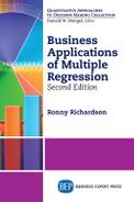
This multiple regression run is shown in Figure 4.1. In this case, the hypotheses for the partial F-test are the following:
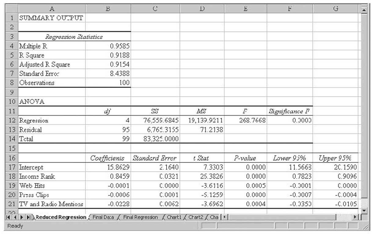
Figure 4.1 The multiple regression run for the reduced celebrity model
H0 : β2 = β5 = 0
H1 : β2 ≠ 0 and/or β5 ≠ 0
The partial F statistic is F distributed with r,n – (k + 1) degrees of freedom where r is the number of variables that were dropped to create the reduced model (two in this case), n is the number of observations, and k is the number of independent variables in the full mode. With α = 0.05 and 2,93 degrees of freedom, the value of the F statistic is 3.0943.
The partial F-test statistic is based on the sums of squares (SSE) for the reduced and full model and the mean square error (MSE) for the full model. It is computed as follows:
Where SSER is the SSE for the reduced model, SSEF is the SSE for the full model, r is the number of variables that were dropped to create the reduced model, and MSEF is MSE for the full model. For the previous examples, the partial F-test statistic is the following:

Because 3.49 is greater than the critical value of 3.0943, we reject the null hypothesis and conclude that either β2 or β5 or both are not zero. This was to be expected because we had already concluded that β5 was not equal to zero.
Partial F Approaches
The partial F-test can be carried out over any combination of variables in order to arrive at a final model. As you can imagine, this would be very tedious and is usually automated by a statistical package. There are four overall approaches that a statistical package can take to select the variables to include in the final model:1
1. All possible combinations of variables. The computer simply tries all possible combinations of k independent variables and then picks the best one. If we are considering k independent variables, then there are 2k–1 possible sets of variables. Once all the possible models are computed, the best one is selected according to some criteria, such as the highest adjusted r2 or the lowest MSE.
2. Forward selection. The computer begins with the model containing no variables. It then adds the single variable with the highest significant F statistic. Once a variable has been added, the computer looks at the partial F statistic of adding one more variable. It then adds the one with the highest F value to the model, as long as that variable meets the significance requirement (e.g., α = 0.05). Once added, this, and all the variables that are added later, remains in the model. That is, once in, a variable is never discarded. The process continues until no more variables are available that meet the significance requirement.
3. Backward elimination. The computer begins with the model containing all the variables. It then computes the partial F statistic for dropping each single variable. It then drops the variable that has the lowest partial F statistic. This continues until all the variables remaining in the model meet the significance requirement. Once a variable is dropped from the model, it is never considered for reentry into the model.
4. Stepwise regression. This is a combination of forward selection and backward elimination. The weakness of these two approaches is that they never reevaluate a variable. Stepwise regression begins as forward selection, finding the single variable to put into the model. It then goes on to find the second variable to enter, as always, assuming it meets the significance requirement. Once a second variable enters the model, it uses backward elimination to make sure that the first variable meets the criteria to stay in the model. If not, it is dropped. Next, it uses forward selection to select the next variable to enter and then uses backward elimination to make sure that all the variables should remain. This two-step approach assures us that any interaction (multicollinearity) between variables is accounted for. The process continues until no more variables will enter or leave the model. Stepwise is the most common approach to deciding on the variables that are to remain in the model.
Forward, backward, and stepwise selection can be seen in operation in Box 4.1.
When working with a large number of variables, model building can be difficult and time-consuming with Excel. This is the situation when there is a real business case for investing in a powerful statistical package like SPSS.
Forward, Backward, and Stepwise Regression in SPSS
The following shows the results of using a statistical package called SPSS to perform forward, backward, and stepwise regression on the data in the SellingPrice.xls worksheet. This worksheet is discussed in more detail a little later in the chapter.
Forward Selection
With this approach, SPSS begins with the model containing no variables. It then adds the single variable with the highest significant F statistic.
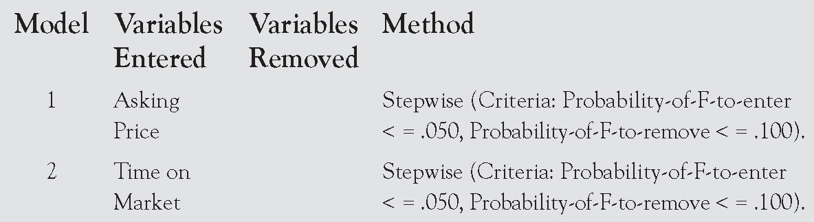
Variables Entered and Removed
Its first report, shown below, shows the variables that have entered the model and the order in which they entered. In this case, the first variable to enter was Asking Price and the second to enter was Time on Market.

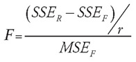
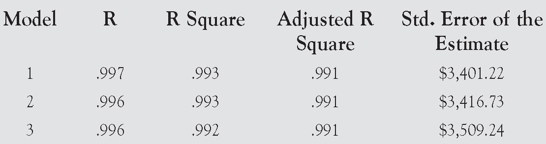
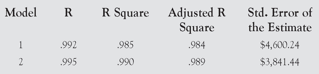
Model Summary
Its next report, shown here, summarizes each model as it is being built. The report shows the r, r2, adjusted r2, and standard error of the estimate for each model.
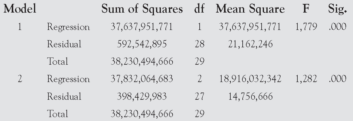
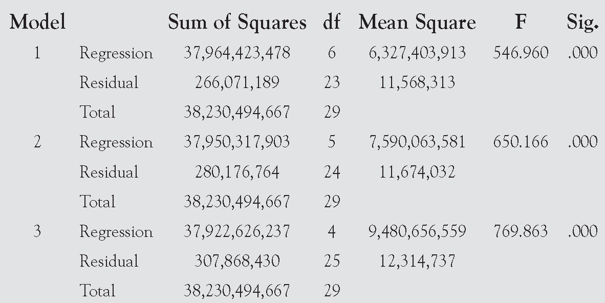
ANOVA
Its next report, shown here, shows the ANOVA table for each model as it is being built.
Coefficients
The next report shows the coefficients for each model as the model is being built.

The final model is represented in the following equation:
Price = $11,536.825 + (0.888 × Asking Price)
–(273.687 × Time on Market)
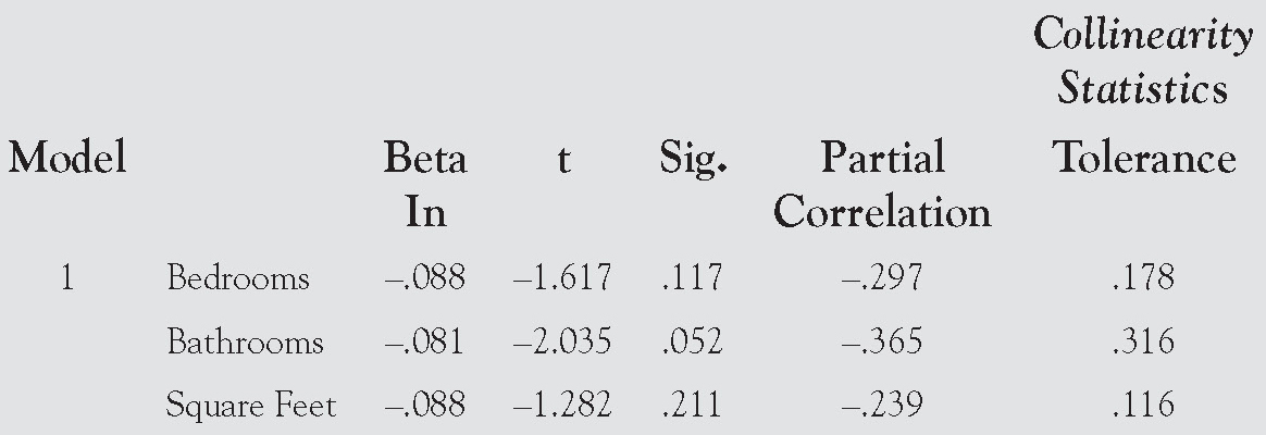
Excluded Variables
The final report shows the variables that were excluded from each model.


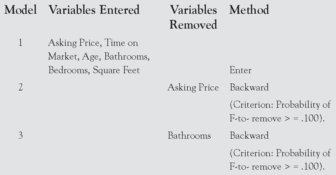
Backward Selection
With this approach, SPSS begins with the model containing all the variables. It then computes the partial F-statistic for dropping each single variable. It then drops the variable that has the lowest partial F-statistic. This continues until all the variables remaining in the model meet the significance requirement. The reports on this method, using the same data, are shown on the pages that follow.
Variables Entered/Removed
Model Summary
Coefficients
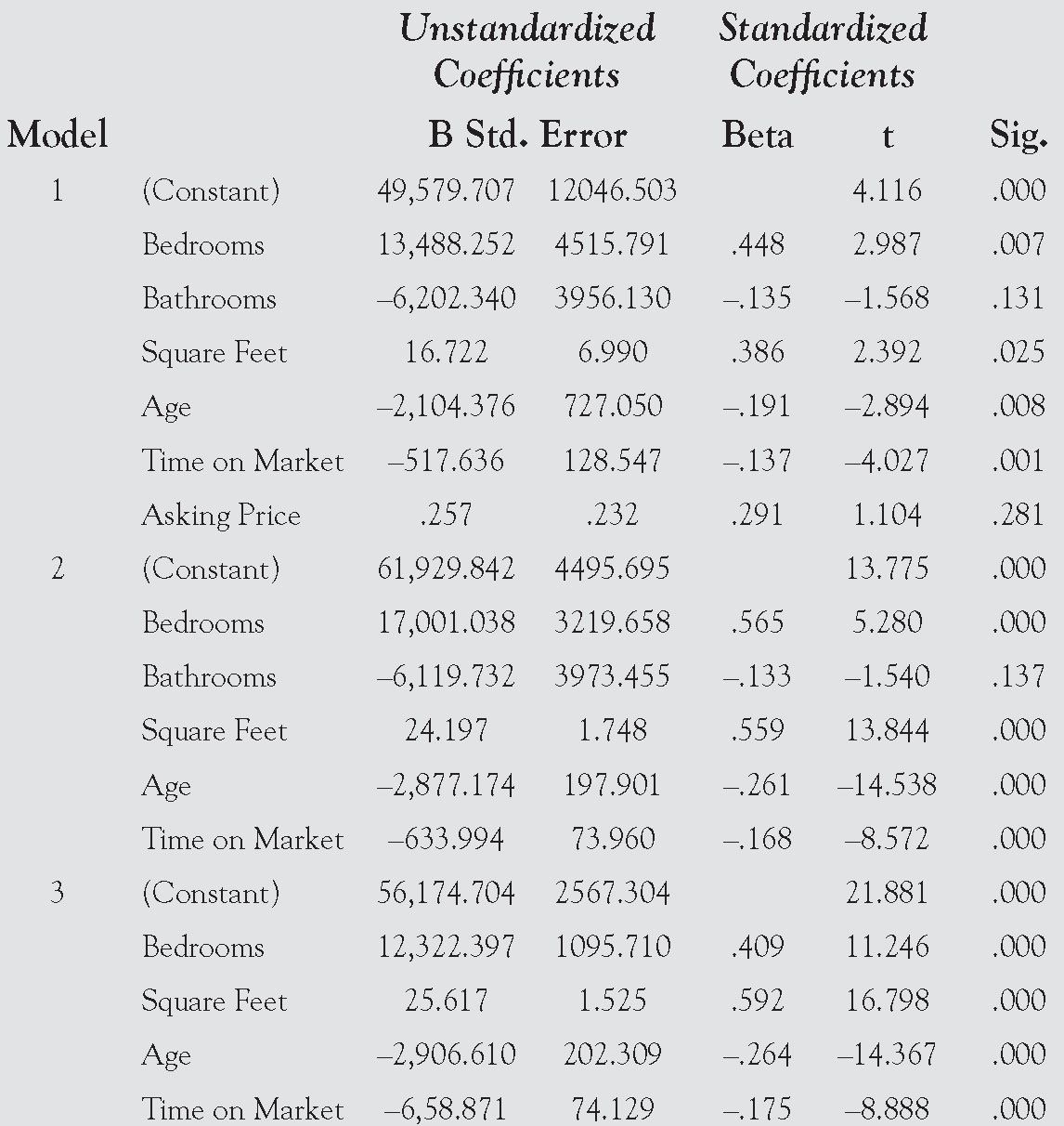
In this case, the final model is represented in the following equation:
Selling Price = 56,174.704 + 12, 322.397 (Bedrooms)
+ 25.617(Square Feet) – 2,906.610(Age)
– 6,58.871(Time on Market)
This is the same model we will end up developing when we approach this problem using Excel. This is to be expected, as the approach we will be using closely mirrors backward selection. Note that this model is very different from the model that was built using forward selection.
Excluded Variables

Stepwise Regression
Using this approach, SPSS finds the single variable to put into the model. It then goes on to find the second variable to enter, as always, assuming it meets the significance requirement. Once a second variable enters the model, it uses backward elimination to make sure that the first variable meets the criteria to stay in the model. If not, it is dropped. Next, it uses forward selection to select the next variable to enter and then uses backward elimination to make sure that all the variables should remain.
Variables Entered/Removed
ANOVA

Coefficients

Using stepwise regression, the model developed matches the forward selection method. This is, of course, not always the case.
Excluded Variables

Summary
The advantage of using any of these approaches in SPSS, rather than building the model manually in Excel, is that SPSS completely automates the process. You simply select the approach to use and SPSS does everything else for you.
None of these four methods for building a model guarantees that we will find the one best model. Because the order of testing can make a difference, it is possible, though not likely, that changing the order in which the variables are entered into the computer will change the results.
Model Building Using Excel
Unfortunately, Excel is not able to automate, or even easily perform, any of the four model-building approaches discussed previously. For this reason, it is always best to work with a dedicated statistics package when trying to develop complex multiple regression models. However, not everyone has access to a dedicated statistics package, as they can be expensive and difficult to use.
To compensate for Excel’s inability to automate building regression models, the author has developed an approach to model building in Excel that approximates backward elimination only using the r2 value that Excel displays rather than the partial F that we would otherwise have to manually compute for each regression run. For models with fewer numbers of observations, the adjusted r2 can be used in place of r2 in making the decisions. This approach has been found to work well on actual data, but its application can be long and tedious when a model has more than a couple of insignificant variables. To make matters worse, none of the steps can be automated. To make matters worse still, the Excel requirement of having the independent variables in contiguous columns causes a good deal of data manipulation problems. For these reasons, readers with complex regression problems are again encouraged to use a statistical program like SPSS or SAS to tackle these more complex problems.
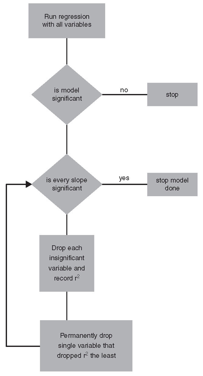
The steps for model building in Excel are as follows:
1. Run the regression with all the variables in the model. If the overall model is insignificant, then stop. When this happens, none of the individual variables will be significant, so there is no point continuing. This is not caused by any violation of regression assumptions. This is usually caused by an error in the theory used to select the variables or, less likely, by a problem with the data, such as having outliers in the data.
2. Test each slope coefficient using the Student t-test. If all the slope coefficients are significant, then stop; you have the final version of the model.
3. If some of the variables are insignificant, make a list of all the insignificant slope coefficients.
4. One at a time, drop a single variable from this list and rerun the multiple regression. Record the resulting r2 and then reinsert the variable into the data set.2
5. Once you have dropped all the insignificant variables one at a time, look at all the r2 values you have recorded. For the run with the highest r2, permanently drop that variable from the data set. That is, drop the variable whose absence causes the least reduction in explanatory power. This variable will be dropped forever and will not be reconsidered for reentry into the model. To do otherwise would be to greatly overwork the problem.
6. Rerun the multiple regression without the variable permanently dropped in step 5. If all the variables are significant, then stop; you are finished. If not, then return to step 2 and continue until all the slope coefficients are significant. The steps for model building in Excel are illustrated visually by the flowchart on page 117.
Selling Price Example
Understanding the real estate market is a common use of regression, a use we will explore in the following example. This example also illustrates using Excel to perform model building. The worksheet SellingPrice.xls contains fictitious data where the dependent variable is the selling price of a house and the independent variables are the following:
• The number of bedrooms
• The number of bathrooms
• The size of the house in square feet
• The age of the house in years
• The time the house was on the market before being sold, in months
• The initial asking price
This is the same data set that was used to illustrate various approaches to multiple regression using SPSS in Box 4.1. The data are shown in Figure 4.2 and the initial regression run is shown in Figure 4.3.
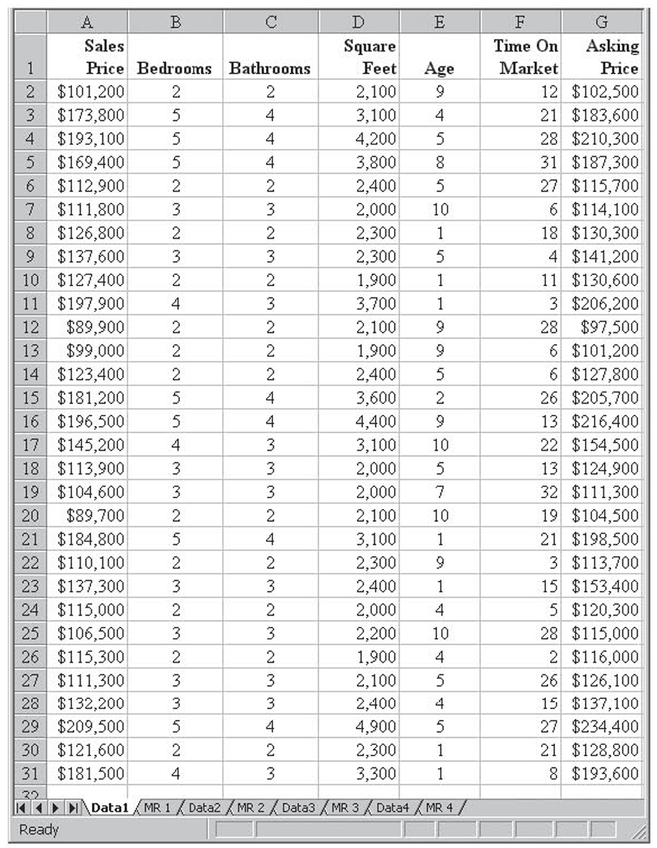
Figure 4.2 The selling price data

Figure 4.3 The initial regression run on the selling price data
To simplify matters and allow us to use the p-value for all the slope coefficients, we will assume that all the slope coefficient hypothesis tests are two-tailed tests. Using these criteria, Figure 4.3 shows us that the following variables are not significant:
• The number of bathrooms
• The initial asking price
So we must drop each variable, in turn, and record the resulting value of r2. Rerunning the regression and dropping number of bathrooms shows us the problems of using Excel to perform more than one multiple regression run on the same data. Specifically, there are two problems: one more serious and one less so.
The more serious problem is that Excel requires independent variables to be in contiguous columns and the number of bathrooms is in the middle of the data set. In order to meet the contiguous columns requirement, we must move the number of bathrooms data out of the way and then either delete the now blank column (if there is nothing else above or below it) or move the remaining data over to remove the blank column.
Due to the chance of deleting other parts of the worksheet while doing this or accidentally deleting part of your data, the author recommends that you take two steps to protect yourself. First, move the regression data to its own worksheet tab so there is no chance of damaging other data with while you move data and delete columns. Second, before you begin, make a backup copy of your data on a second worksheet tab. That way, if you accidentally delete data, you can go to this backup sheet and recover it.
The less serious problem is that the regression function in Excel remembers your last set of inputs and has no reset button. That means you must remember to manually change the setting for the independent variables and output sheet each time you run regression.
Dropping Number of Bathrooms results in an r2 value of 0.992. That regression run is shown in Figure 4.4. We now put back in the Number of Bathrooms and drop the Initial Asking Price. Dropping the Initial Asking Price results in an r2 value of 0.993. That regression run is shown in Figure 4.5.

Figure 4.4 Dropping number of bathrooms from the model
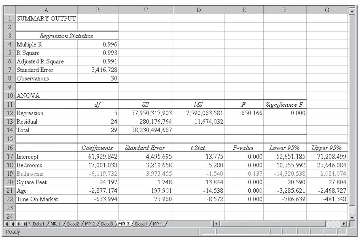
Figure 4.5 Dropping asking price from the model
Dropping the Initial Asking Price results in a higher value for r2. (0.993 versus 0.992), so Initial Asking Price is permanently dropped from the model. This run is shown in Figure 4.5. Number of Bathrooms remains insignificant in this model, but now it is the only insignificant variable so it is dropped from the model without any testing. Those results are shown in Figure 4.6.

Figure 4.6 The final model with both Number of Bathrooms and Asking Price dropped from the model
In this final version of the model, all the variables are significant. The overall r2 has only dropped from 0.993 in the original model to 0.992 in this final model. As expected, dropping insignificant variables had little impact on r2.
In this example, all the variables that were insignificant in the original model ended up being dropped from the final model and no additional variables were dropped, so you may be wondering why it was necessary to work through this process. As will be demonstrated with a later model, this is not always the case. Because we cannot usually tell in advance when significance will change as variables are dropped, it is always necessary to go through this process when more than one variable is insignificant.
Before we move on, we will take a moment to consider this model from a business, rather than a statistical, standpoint. How might a model like this be used? One possible use is appraisal. Because the model quantifies the selling price of a house based on the house’s attributes, an appraiser (tax appraiser or loan appraiser) can plug in the attributes of a house under consideration and get an estimate of the value of that house. That estimate is not exact because things like condition and aesthetics also play a role, but it is a good starting point.
Likewise, a homeowner considering making an addition such as adding a bedroom, or a contractor trying to sell an addition, could use the model to estimate the improvement in the value of that addition. This, in turn, might affect what the homeowner is willing to pay or the contractor is able to charge.
Box 4.2
Using Regression to Schedule Meter Reading
Scheduling service personnel is very difficult when the services they perform are not routine. For example, scheduling calls for a plumber or cable repair person requires that you have at least a good estimate of how long each job will take and how long the travel between jobs will take. However, job time varies greatly depending on the specific situation of the job, and travel time can vary greatly depending on the time of day. We will explore these issues by way of an example from the electric utility industry. Although the resulting model is specific to the electric utility industry, the approach and techniques generalize to a great many service industries.
Electric utility companies must periodically read their customer’s electric meter for billing purposes. Even in this high-tech world, many electric utilities get those readings by sending a meter reader out to walk through residential neighborhoods and commercial areas to physically look at each meter and record its readings. Research is ongoing on techniques for having the meters send their readings back to a central computer automatically, either over the power lines or via a cell phone network, but for many companies, physically reading the meters each month is cheaper.
One utility company reads meters on a 21-day cycle. That is, a meter reader reads one new route each day for 21 working days and then starts the set over again. With weekends and holidays, this 21-day cycle results in the customer getting a bill about once a month. The collection of meters that is read by a meter reader on a given day is called a route. Routes remain static for, on average, 2 years and each meter reader keeps the same set of 21 routes during this 2 years. This allows the meter readers to become familiar with their routes. When new construction takes place, those meters are added to the nearest route. Because new construction is rarely evenly dispersed, this results in some routes growing much more than other routes. Every 2 years, each meter reading office reroutes—that is, they reallocate meters among routes to try to level the workload.
In this box, we will work with actual meter-reading data from a utility company and see how multiple regression can take that data and develop a model that can be used to estimate (i.e., forecast) the time that would be required by any set of meters. This can make the rerouting process much easier and can result in routes that, at least at the start of the 2-year period, have the workload more equally distributed.
This utility company is divided into districts, and many of the districts are divided into local offices. Each local office has an assigned area for meter readings, as well as other tasks. Meter-reading routes never cross local office or district lines so the process of rerouting is constrained to optimizing the routes within each local office independently. Additionally, because each meter reader reads 21 routes, each local office can have either 21 routes, 42 routes, or 63 routes, and so on.
Another major consideration in designing routes is how hard to make the routes. Meter readers are expected to read meters for 6 hours per day. They have 1 hour in the morning to get their paperwork ready and drive to the start of their route. At the end of the day, they have 1 hour to drive back to the office, process their paperwork, and turn in any money they collected for past-due bills. Thus do you design the routes so that only an experienced meter reader who is familiar with the route and working in good weather can possibly finish it in 6 hours, or do you design the routes so an inexperienced meter reader who is unfamiliar with the route and working in poor weather has time to finish? If you choose the former, then many routes will not be finished. If you choose the latter, then experienced meter readers on familiar routes working in good weather will finish in well under 6 hours.
The term “route” is somewhat misleading. When reading a route, a meter reader will walk between consecutive meter locations if they are close together, as is usually the case for residential meters. If consecutive meters are located a considerable distance apart, as is sometimes the case with commercial meters, the meter reader will use a company-furnished automobile to drive between meter locations. However, one route does not have to be all walking or all driving. Most neighborhoods and commercial office parks are too small to take a meter reader all day to finish. Typically, a meter reader will read meters in one area for a time, then drive to another area and begin reading again. A route then may consist of two, three, or even more route segments.
The Data
The data used in this analysis were collected from experienced meter readers who were reading routes with which they were familiar. When a route consisted of more than one segment, each segment was measured and recorded individually. When anything unusual happened that significantly changed the reading time for that segment, that observation was dropped from the data set.
Additionally, certain routes have special circumstances that require significant amounts of time and are always a factor. For example, one of the meters at a local airport is on a radio tower on the opposite side of a controlled runway. To read this meter, the meter reader must go to the Federal Aviation Administration (FAA) office at the airport tower and request that an FAA person drive him across the runway in an FAA car. Once the FAA car is at the runway, both going and coming back, the operator must contact the control tower and wait for clearance to cross the active runway. As you can imagine, this greatly increases the time required to read this meter. Although few meters take this long to resolve, any route segment with a regular special circumstance was excluded from this analysis.
The variables collected for this analysis are explained next. Although other variables might have been more helpful, this set was selected because it either was available from information already stored by the utility company or was easy to measure for a given route segment.
Time. This is the time required by each meter reader to read a given route segment, recorded in minutes. Utility company meter readers use handheld computers to enter the meter readings, and these record the time the reading was entered so the time for a route segment could be calculated as the time for the last reading minus the time for the first reading.
Number of residential (or nondemand) meters. Electric meters fall into two major categories: nondemand and demand meters. Nondemand meters have a continuously moving display showing the number of kilowatt-hours of electricity that have been consumed since the meter was installed. If the reading last month was 40,000 and the reading this month is 41,200, then 1,200 kilowatt-hours were consumed between the two readings. With a nondemand meter, the meter reader simply records the reading and continues on. Nondemand meters are used almost exclusively for residents, although small business applications—roadside signs, apartment laundry rooms, and the like—might also use nondemand meters. Nondemand meters are quick to read.
Number of demand meters. Demand meters, on the other hand, take much longer to read. Like a nondemand meter, demand meters have a kilowatt-hour consumption meter that must be read and recorded. However, they also have a second meter, the demand, that records the peak consumption for the last month. Because this meter records a peak, it must be reset each month in case the following peak is lower. The demand is a significant part of a commercial electric bill so, to keep the customer from resetting the peak, the reset knob is locked with a color-coded plastic seal. After reading and recording the peak, the meter reader must break the seal, reset the meter, and install a new seal of a different color. Naturally, reading a demand meter takes significantly longer than reading a nondemand meter. Additionally, business meters (i.e., demand meters) tend to be further apart than residential meters (i.e., nondemand meters), a fact that the regression model will also consider.
Number of locations. Reading 100 meters in an apartment complex with 20 meters per building would take less time than reading 100 meters on the sides of 100 houses. This variable records the number of separate locations for each route segment.
Number of collects. When a residential electric bill is 2 months past due, this utility company expects its meter readers to try to collect for that bill as they read their routes. They are given bill collection cards in the morning that they must sequence into their routes. These cards are marked as either collects or cuts. With a collect, the meter reader knocks on the door and requests payment. If payment is given, then the meter reader collects that money and gives them a receipt. If no one is home, the meter reader leaves a preprinted note on the door. If the customer refuses to pay or is not home, no other action is taken.
Number of cuts. If the card is marked as a cut, then all the previously mentioned steps take place, but if the meter reader does not receive payment for any reason, he cuts off power to that house. This is done by cutting a seal on the meter box, removing the meter box cover, pulling out the electric meter, putting plastic sleeves on plugs on the back of the meter, reinstalling the meter, reinstalling the face plate, and locking the meter. As complicated as it sounds, it can be completed in under 60 seconds by an experienced meter reader. Although the number of collects and cuts will vary month to month, some routes are statistically much more likely to have a higher number of collects and cuts than are others. Interestingly, this is not always related to the average income of the neighborhood. Meter readers only attempt collections and cut off power for residential customers. Collections and cutoffs of commercial and other classes of customers are handled by a special bill collector.
Miles walked. It would be nice to know the real number of miles a meter reader needed to walk for a route. Residential meters can be on the front, on either side, on the back of a house, or even in the basement. This requires walking up the front yard, perhaps down one side, and perhaps around the back of the house. Commercial meters can be located anywhere around a building or in a power room or maintenance room inside or even on the roof. Measuring all these distances would take too long and would require the cooperation of all the meter readers. Miles walked then is a surrogate. It is simply the mileage as measured by driving a car down the street along the route. Naturally, the miles walked by the meter reader would be greater than this, but regression can account for this.
Miles driven. When a route segment must be driven, this is simply the mileage recorded using the automobile odometer. This does not include travel to and from the route because that is not part of the 6 hours allotted to meter reading.
There are a number of additional factors that can affect meter-reading times on a route. These considerations are best classified as random variations or white noise in the meter-reading process. No effort was made to quantify or measure these. Examples include the following:
• Unfriendly dogs. An aggressive dog inside a fence is a problem when the electric meter is inside that same fence. The meter reader must either try to coerce the dog into allowing him entry or take the time to knock on the door and get the owner to control the dog while he reads the meter. An aggressive dog running loose can cause the meter reader difficulty for any number of houses.
• Fences. Fenced yards require more walking to gain access through the gates or the meter reader must climb over the fence. Locked gates only exacerbate this problem.
• Bushes. Bushes make it hard to get close to meters and to see them.
• Traffic. While on the driving portion of a route, traffic can delay the meter reader.
Experience indicates that the variations affect many routes in a fairly random fashion. For this reason, they were not measured or included in this analysis.
Data Analysis
Figure 4.7 shows the top of the data file. The data are stored in the Data tab of the Meter.xls worksheet. Figure 4.8 shows correlation analysis on the independent variables. Multicollinearity is not much of a problem, with only number of locations and miles walked clearing the 0.60 hurdle.
Figure 4.9 shows the initial regression run on the data. The variations in the independent variables explain 85 percent of the variations in the dependent variable. Only the Number of cuts was insignificant, so that variable was dropped from the analysis. Figure 4.10 shows the resulting regression. This time, all the variables are significant, and still about 85 percent of the variation is explained.
This gives this resulting regression equation:
Resulting Regression Equation
Times to Read Route (Minutes) = 10.2563 + 0.1596 (Number of Residential Meters) + 0.4439(Number of Commercial Meters) – 0.0834(Number of Locations) + 2.2049(Number of Collects) + 29.7468(Miles Walked) + 4.0522(Miles Driven)
Because Time was measured in minutes, this equation tells us that adding 1 residential meter to the route, while holding everything else constant, would add about 10 seconds (0.1596 × 60 seconds) to the time it takes to read a route, whereas adding a commercial meter would add about 27 seconds. Each collect adds a little over 2 minutes, each mile walked adds almost half an hour, and each mile driven adds a little over 4 minutes.
What is harder to understand, at first, is why the coefficient for Number of locations is negative. After all, adding more locations should increase the work. Recall, however, this is adding one location while holding everything else constant. That means no additional meters and no additional walking, so increasing the number of locations reduces the meter density and implies that the meters must be closer together because walking mileage does not change. This complexity is likely the reason for the negative coefficient, and its magnitude is so small that it has little impact on the results so it also could just be a statistical anomaly.
The resulting equation uses only easily obtainable data for each route. Using this equation would give management an easy way to manipulate route contents during a rerouting in such a manner that the resulting routes require very similar times to complete. This should lead to greater equality among the meter-reading employees and less dissatisfaction.

Figure 4.7 The top of the data file for the meter-reading data. The full data set has 121 observations
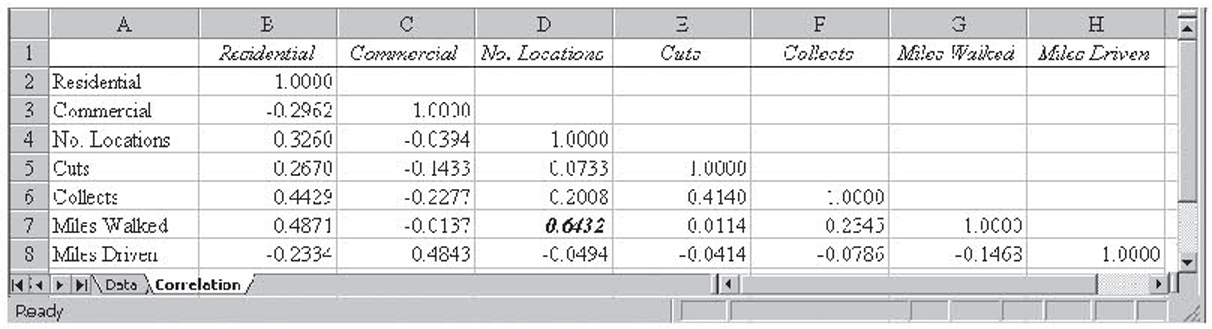
Figure 4.8 Correlation analysis results on the independent variables for the meter-reading data
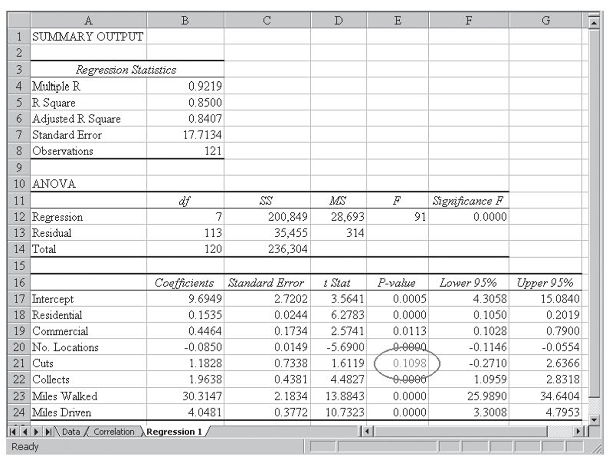
Figure 4.9 The initial regression results on the meter-reading data

Figure 4.10 The final regression results on the meter-reading data
Including Qualitative Data in Multiple Regression
So far, all the variables that we have used in multiple regression have been ratio-scale data. Some of them, such as square feet in the last model, have been continuous, whereas others, such as number of bathrooms in the last model, have been discrete, but they have all had meaningful numbers attached to them. In this section, we will see how to include qualitative data in multiple regression. For example, in the sales model we have mentioned several times, you might want to include whether a competitor is having a sale in the model. This is an example of a qualitative variable because there is no meaningful number that can be attached to the yes or no answer to if the competitor is having a sale.
Qualitative data are very useful in business. We might want to indicate the make of the machines in a model to predict when maintenance is required, we might want to include the season of the year in a model to predict demand, or we might want to include a flag when demand was influenced by a special event. All of these situations can be handled in the same way.
When only two possible conditions exist, such as with gender or the presence or absence of a special event, we use a special variable in the regression model. This variable goes by several names: dichotomous variable, indicator variable, or dummy variable. The dummy variable takes on a value of one when the condition exists and a value of zero when it does not exist.3 For example, we would use a value of one when the special event happened and a value of zero for those periods where it did not happen.4 For gender, we would arbitrarily choose either one or zero for male and use the other value for female.
Once the dummy variable is defined, no other special considerations are required. We run the multiple regression the same way, we test overall significance the same way, and we decide which variables to keep and which to discard exactly the same way. Dummy variables can be dropped for insignificance just like any other variable. An example follows.
Dummy Variable Example
The worksheet Dummy.xls contains fictitious data on two models of machines, a Wilson and a Smith, along with their average hours between breakdown and their age. These data are shown in Figure 4.11. By coding the Smith as a zero and a Wilson as a one, these data can be used in multiple regression. The coded data are shown in Figure 4.12, and the resulting data are shown in Figure 4.13. Note that the dummy variable we created is significant in the model, as is the age of the machine.

Figure 4.11 The original data set with the machine name

Figure 4.12 The modified data set with the machine name coded using a dummy variable
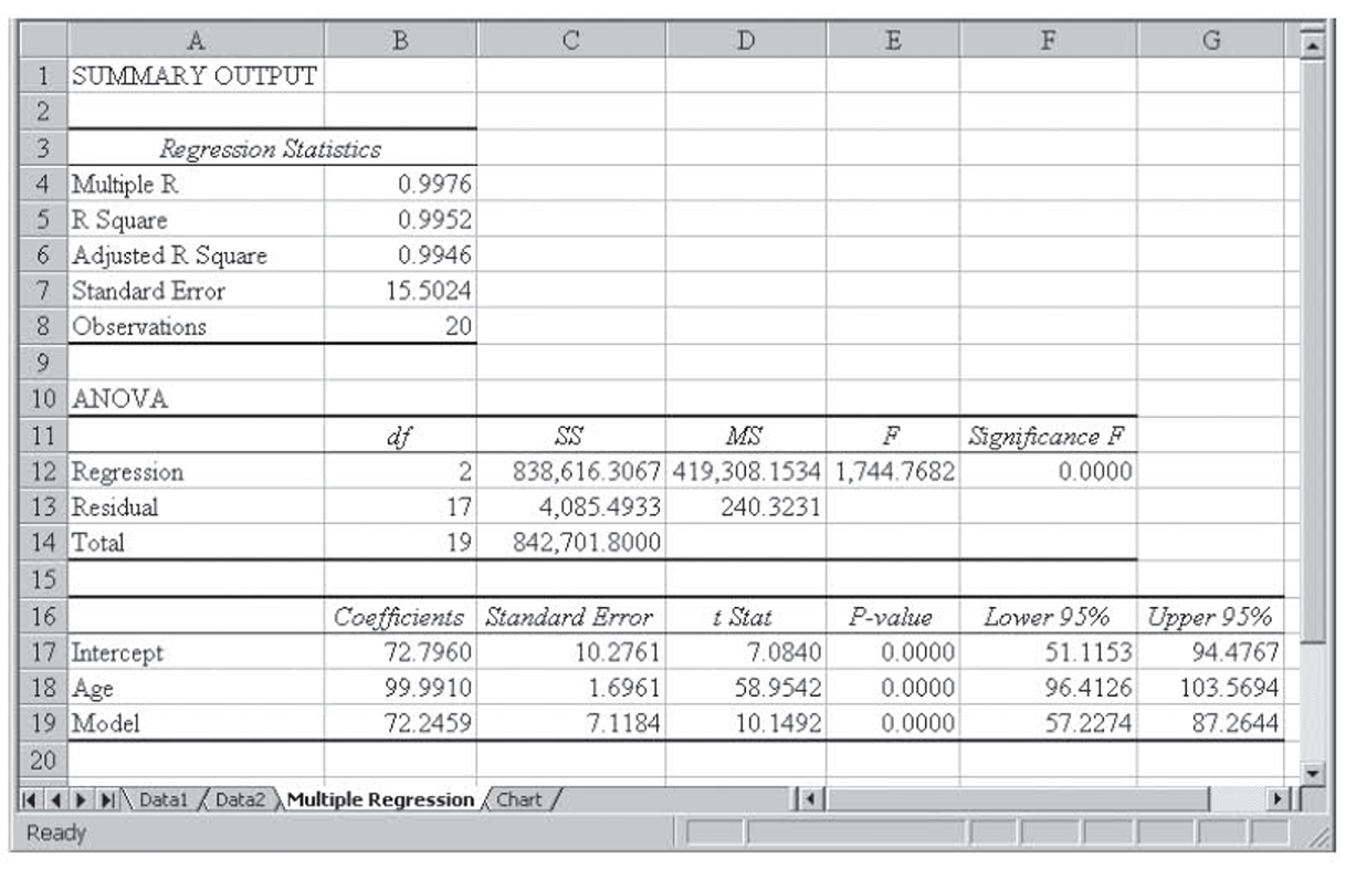
Figure 4.13 The resulting regression run
Including a dummy variable in multiple regression causes the intercept to shift and nothing more. For this reason, dummy variables are also called intercept shifters. This can best be seen using the previous example.
Dummy Variable Example Continued
From Figure 4.13, we get the following regression equation:
Regression Equation
Hours Between Breakdown= 72.7960 + 99.9910(Age) + 72.2459(Model)
However, Model can only take on the values of either zero or one. Substituting these values into the equation, we get the following:
Regression Equations Considering Dummy Variable
When Model = 0,
Hours Between Breakdown= 72.7960 + 99.9910(Age) + 72.2459(0),
which reduces to
Hours Between Breakdown= 72.7960 + 99.9910(Age).
When Model = 1,
Hours Between Breakdown= 72.7960 + 99.9910(Age) + 72.2459(1),
which reduces to
Hours Between Breakdown= 72.7960 + 99.9910(Age) + 72.2459,
which finally reduces to
Hours Between Breakdown= 145.0419 + 99.9910(Age).
Thus the only difference between the two equations is the intercept. Figure 4.14 illustrates this using a chart.
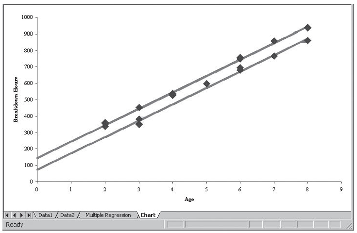
Figure 4.14 Charting the two regression lines, one when the dummy variable is zero and the other when the dummy variable is one
More Than Two Possible Values
Of course, many times we wish to include a qualitative variable in the model that has more than two possible conditions. Examples might include race or eye color. We cannot simply define the variable using more than two values for our one dummy variable. For example, it would not be correct to have a dummy variable for competitor sale where 1 = no sale, 2 = minor sale, 3 = major sale, and 4 = clearance sale. The reason is based on the fact that dummy variables shift the intercept. Setting the variable up this way presupposes that the shift in the intercept between no sale and minor sale is the same as the shift between minor sale and major sale and the shift between no sale and minor sale is twice that of between no sale and clearance sale. Of course, we do not know this in advance, and it is likely not the case anyway.
Although we cannot code the single dummy variable in this fashion, we can include this data using multiple dummy variables. In this case, we would need three dummy variables. The first one would be a one for when there was no sale and zero otherwise. The second would be one for where there was a minor sale and zero otherwise. And the third would be one for when there was a major sale and zero otherwise. We do not need a fourth variable for other sales because a zero for all three of these dummy variables would automatically tell us that there must be a clearance sale. In fact, including this fourth, unneeded, dummy variable would force at least one of the dummy variables to be insignificant because any three would uniquely define the fourth. In general, you need n – 1 dummy variables to code n categories. In this case, you end up with n – 1 parallel lines5 and n – 1 different intercepts.
The use of dummy variables when there are a large number of categories can greatly expand the number of variables in use. One of the pieces of information in the author’s dissertation was state. Coding this into dummy variables required 49 (or 50 – 1) different variables. When the number of variables grows in this fashion, you must make sure you have an adequate sample size to support the expanded number of variables. As before, we recommend a minimum of 5 observations for each variable, including each dummy variable, with 10 per variable being even better. This was not a problem for the author because he had over 22,000 observations.
It is also possible to include more than one dummy variable in a regression model. For example, we might want to include both sale types and whether it is a holiday period in our model. When we have multiple dummy variables, each one is coded as described as done previously without consideration of any other qualitative variables that might need coding. That is, we would need one dummy variable for whether it is a holiday period and then three more for sale type, assuming the four categories previously discussed. The result would be a great deal of intercept shifting.
As you can imagine, the list of qualitative data you might need to include in a business model is quite long. Although no means comprehensive, that list includes model number, model characteristics, state or region, country, person or group, success or failure, and many more. Some of these are explored in Box 4.3.
Dummy Variable as Dependent Variable
It is also possible to use a dummy variable as the dependent variable. When you do this, it is not called regression. Rather, it is called discriminate analysis. Other than the name change, discriminate analysis is performed the same way as regression. This is discussed in more detail in Box 4.3.
The Business of Getting Elected to Congress
As stated previously, businesses often need to include a wide range of qualitative data in statistical models. While the following example is not a business example in the truest sense of the word, it does illustrate the use of qualitative data both as a dependent variable and as independent variables.
It takes a lot of money to get elected to Congress. Once elected, it takes a lot of money to stay elected. In this box, we will use a form of multiple regression analysis called discriminate analysis to see what affects who gets elected to Congress. As was described in the chapter, discriminate analysis is nothing more than multiple regression where the dependent variable is a dummy variable. In this case, the dependent variable will be whether they won their election.
The data for this sidebar came from Douglas Weber, a researcher at the Center for Responsive Politics. PresidentialElection.com describes the Center for Responsive Politics as follows:
The Center for Responsive Politics is a non-partisan, non-profit research group based in Washington, D.C. that tracks money in politics, and its effect on elections and public policy. The Center conducts computer-based research on campaign finance issues for the news media, academics, activists, and the public at large. The Center’s work is aimed at creating a more educated voter, an involved citizenry, and a more responsive government.6
The data for this analysis come from the 1996–2000 political campaigns for the U.S. Congress. These data are stored in the Excel file CandidateSpending1996-2000.xls in the Raw Data tab. The top of this data file is shown in Figure 4.15. Altogether, there are 2,086 entries. The variables stored are as follows:
• Cycle. This is the election year. Members of the House of Representatives are elected every 2 years. Members of the Senate are elected every 6 years, but the elections are staggered so some senators are up for election every 2 years. In this data set, the values for cycle are 1996, 1998, and 2000.
• Office. This is the office for which the candidate is running. In this data set, the values are H (House) or S (Senate).
• State. This is the two-digit postal code for the state that the candidate is seeking to represent.
• DistID. This is an identification number for the district from which the candidate is running.
• CID. This is a universal identification number for a candidate that is assigned by the Center for Responsive Politics and that stays constant throughout the candidate’s career.
• Candidate Name. This is the name of the candidate.
• Party. This is the party of the candidate. Most of the candidates are either Democrats (D) or Republicans (R). A few are third-party candidates (3), independents (I), or Libertarians (L).
• Won/Lost. This tells if the candidate won (W) the election, lost (L) the election, or if the election was undecided (U). This variable will end up being the dependent variable.
• CRPICO. This is a code indicating whether the candidate is an incumbent (I), challenger (C), or if the seat is open (O). An incumbent already holds the office for which he or she is running, a challenger runs against an incumbent, and an open election is one where there is no incumbent running.
• Spending. This is how much money the candidate spent on the election.
• Opponent Spending. This is how much money the candidate’s opponents spent on the election.
Many of these variables must be modified or converted before they can be used for discriminate analysis:
• Cycle. This is a numeric variable and can be used as is.
• Office. This variable was converted to a dummy variable, with zero for House and one for Senate.
• State. Different states would reasonably have different spending levels for offices as well as many other likely differences. In a complete analysis, the values for the 50 states would be converted to 49 dummy variables in order to capture those effects. Given Excel’s difficulty in handling large numbers of variables, it was decided to drop the state value from the analysis.
• DistID. This has no statistical value and was dropped for analysis.
• CID. This has no statistical value and was dropped for analysis.
• Candidate Name. This has no statistical value and was dropped for analysis.
• Party. There are five possible values for this variable, so four dummy variables are required. Those dummy variables are Democrats, Republicans, Libertarians, and independents. Of course, any entry with a zero for all four would be a third-party candidate.
• Won/Lost. This is the dependent dummy variable, so it was moved to the left side of the data set to allow the independent variables to be contiguous. A value of one was used for a win, so a zero represented either a loss or an undecided election. Remember that a dummy variable can only have two values (zero and one), and when used as the dependent variable, there can only be one dummy variable, so it was not possible to separate loss and undecided.
• CRPICO. There were three possible values, so two dummy variables are required. They are incumbent and challenger. A zero for both variables indicates an open election.
• Spending. This variable was used as is.
• Opponent Spending. This variable was used as is.
• Ratio. A new variable was created from the ratio of Spending divided by Opponent Spending.
The top of this modified data set is shown in Figure 4.16.
The Analysis
The first step is to perform correlation analysis on the independent variables. Those results are shown in Figure 4.17. Surprisingly, there are only four pairs of variables where multicollinearity is likely to be a problem:
1. Democrat/Republican (–0.9791). This is not surprising because almost all the candidates are either Democrats or Republications, you would expect a near perfect correlation, and we get it. The negative correlation only means that as the Democrat dummy variable goes up from zero to one, the Republican dummy variable moves in the opposite direction, from one to zero. The fact that the value is not exactly 1.00 simply indicates the presence of a few candidates who are neither Democrats nor Republicans.
2. Opponent Spending/Office (0.4835). This does not pass our 0.60 threshold, but given the very small values for the other pairs, it is noticeable. Since Office is a dummy variable with a zero for House and one for Senate, this indicates a strong likelihood that nonincumbent spending is higher for the Senate than for the House. This is not surprising because the Senate is both more prestigious and a statewide seat requiring statewide campaigning.
3. Spending/Office (0.4835). Like opponents, incumbents spend more for the Senate than for the House. What is surprising is that the correlation is the same for both spending variables.
4. Challenger/Incumbent (–0.7678). This is also not surprising because someone who is not a incumbent must be a challenger. The reason for the less-than-perfect correlation is that some of the elections are open elections where there is no incumbent.
The initial regression results are shown in Figure 4.18. Overall, the model is able to explain a little over 70 percent of the variation in the results. No doubt, candidate positions on specific issues and character issues accounted for much of the remaining percentage. Additionally, issues like these no doubt affected the candidate’s ability to raise money, so some of those issues would be reflected in the spending variable.
Cycle is not significant, which seems to indicate that the impact of the various variables has not changed over the relatively short period of time represented in this data set. Office is not significant, indicating that election patterns are fairly consistent for the House and Senate. The Democrat and Republican dummy variables are not significant, which is surprising. This seems to indicate that spending and being an incumbent are much more important than party affiliations. Along the same lines, Libertarian is also not significant, but because there were only seven Libertarian candidates in this period, that is not surprising.
Incumbent was significant with a positive coefficient, as expected. That is, being an incumbent strongly helps your chance of being elected. Along the same lines, being a challenger was also significant and, as would be expected, had a negative coefficient. Spending and Opponent Spending are both significant and both have positive coefficients. They appear to be zero because the dependent variable is either zero or one and spending is measured in dollars and so has values in the millions. This large difference in the units yields very small coefficients. The spending ratio is also significant with a positive coefficient, indicating that the higher a candidate’s spending relative to his opponent’s spending, the better his or her chance of being elected. Again, the magnitude of the spending ratio coefficient is due to the magnitude of the ratios and not to its importance. Note that the largest ratio was over 650.
Normally, we would need to work through these variables, dropping them one at a time, to figure out which to drop. That work has been done but is not shown. All the variables that are insignificant in the first model end up dropping out of the final model, although when either the Democrat or Republican dummy variable is left in, whichever variable that is left in is almost significant.
Additionally, the two spending variables were both divided by 1,000,000, yielding spending expressed in millions of dollars. This is a linear transformation, so it has no effect on correlation or r2 but does keep the coefficients for the spending variables from being so small. Also, transforming the spending variables has no effect on their ratio, so that variable stays the same. While not shown in a figure, this reduced data set is stored in the Data2 tab of the worksheet.
The regression on this final, reduced data set is shown in Figure 4.19. Notice that everything is significant. Variations in these six variables explain 70 percent of the variation in who won the election. This gives the following equation:
Final Regression Equation
Y = 0.49609 + 0.42575(Incumbent) – 0.43639(Challenger) + 0.01684(Spending, in millions) – 0.01616(Opponent Spending, in millions) + 0.00080(Ratio)
All these variables have the sign that we would expect.
If we are careful, in discriminate analysis, then it is possible to use the magnitude of the final coefficients to analyze the relative impacts of the independent variables. Great care is required because the magnitude of the coefficients, which is what we will be analyzing, is greatly influenced by the units in which the variable was measured. Of course, not all variables have a problem with units, as will be seen.
Understanding the Coefficients
Recall that our dependent variable was a dummy variable that had a value of one if the candidate won the election and a value of zero if the candidate lost the election. While all the observations in the data set have a value of zero or one for this variable, the resulting regression equation is not restricted to this 0–1 range. When this regression equation was applied to the 2,086 observations in this data set, on the Forecast tab, values for the forecasted dependent variable ranged from –0.43 to 1.47. Nevertheless 2,051 of 2.086 (98.3 percent) of the forecasts did fall within this range. Some of these results are shown in Figure 4.20.
Everything else being equal, the closer a candidate’s score is to one, the higher the likelihood that they will win the election. Likewise, the closer a candidate’s score is to zero, the lower the likelihood that they will win the election. So the forecast that results from the regression equation can roughly be treated as a probability of winning. This is only a rough approximation because 30 percent of the variation is unexplained and because values below zero or greater than one are possible.
The intercept is 0.49609 or very nearly 50 percent. This is exactly what we would expect. Without considering money or whether or not a candidate is an incumbent, with two strong parties, a candidate should have about a 50-50 chance.
Recall from above that the Democrat variable is almost significant. If it is left in for the final regression, none of the above coefficients changes more than a minor amount, and the Democrat variable has a coefficient of 0.02079. That is, during the time range associated with this data set, being a Democrat has a small (0.02079) positive impact on the probability of winning. Of course, one of the problems with handicapping political races using historical data is the 2002 elections, where being a Democrat had a negative impact. Because the data we are analyzing stops at 2000, the impact of the 2002 elections is not included. This illustrates the difficulty of using historical data to forecast elections.
Being the incumbent had a large (0.42575) positive impact on the probability of winning, while being a challenger had a large (–0.43639) negative impact on the probability of winning. Recall that spending is now measured in millions of dollars, and spending an additional one million dollars has only a small (0.01684) impact on the probability of winning. Of course, had spending been measured in tens of millions of dollars, the coefficient would be larger (0.1684), but the overall impact of spending would be the same, thus the caveat regarding the units used to measure the variables. Opponent spending had about the same impact (–0.01616 versus 0.01684) for a million dollars spent, thus candidate and opponent spending tend to offset one another. The ratio of opponent spending has only a minor impact (0.00080) on the probability of winning, so it takes a large imbalance to cause a large swing in the probabilities. Of course, these data are all for national offices with very large spending levels. This observation is not likely to be true for state or local elections with their relatively small budgets.
Conclusion
This box has shown how election data can be used to build a model for predicting the relative chances of a political hopeful being elected to Congress based on the candidate’s and the candidate’s opponent’s incumbent and spending status. The resulting model was able to explain about 70 percent of the variation.
Now imagine that, rather than political data, this worksheet contained income, debt, and spending data on consumers. Also imagine that rather than election results, the dependent variable was a dummy variable where one represented a good credit risk and zero represented a bad credit risk. If that were the case, then column A in Figure 4.20 could contain credit scores rather than electability scores. Statistical analysis of credit history similar to what is presented here is, in fact, exactly how credit scores are developed.

Figure 4.15 The top of the candidate data file

Figure 4.16 The top of the candidate data file after the modifications discussed have been made

Figure 4.17 Correlation analysis of the independent variable in the candidate data file
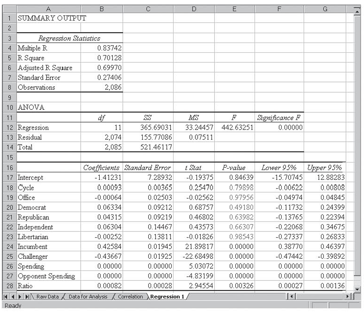
Figure 4.18 The initial regression run

Figure 4.19 The final regression model for the candidate data file
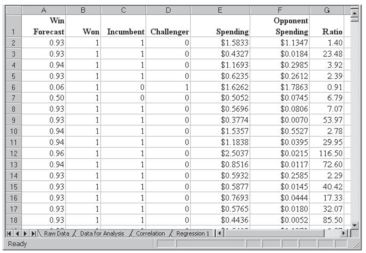
Figure 4.20 Forecasting winning using the candidate data set
Because regression, and therefore discriminate analysis, can have only one dependent variable, it is only possible to use a dummy variable as the dependent variable when you only have two possible categories, such as repaying a loan (or not) or making a sale. These types of models are often used by financial institutions where the dummy dependent variable represents whether someone is a good credit risk. The purpose of discriminate analysis is to assign each observation into one of the two categories described by the dependent variable. In other words, we wish to discriminate between the two possible outcomes. The development of this type of model is left to interested readers.
Because regression can only have one dependent variable, regression-based discriminate analysis can only support two categories. There are more advanced approaches for handling more than two categories. Interested students are referred to an advanced reference.
Testing the Validity of the Regression Model
There are three main problems, or diseases, that can affect multiple regression:
1. Multicollinearity
2. Autocorrelation
3. Heteroscedasticity
We will look at spotting and treating each of the problems individually.
Multicollinearity
Multicollinearity is a major problem that affects almost every set of data to some degree. It is the sole reason we cannot just drop all the insignificant variables at once. As we will see, it can also cause coefficients to be hard to understand, as well as an array of other problems. Were it not for multicollinearity, developing multiple regression models would be an order of magnitude easier.
The best way to see the impact of multicollinearity is to see how well multiple regression performs without multicollinearity. An example of this follows.
Example With No Multicollinearity
Figure 4.21 shows a data set that has one dependent variable, Y, and four independent variables, X1 through X4. The independent variables were constructed such that they have absolutely no multicollinearity.7 Because multicollinearity is correlation between the independent variables, the quickest way to test for multicollinearity is via a correlation matrix containing just the independent variables. This is shown in Figure 4.22. As you can see, no correlation, and therefore no multicollinearity, is present.

Figure 4.21 Made-up data set containing no multicollinearity

Figure 4.22 Results of running correlation analysis on this fictitious data set that contains no multicollinearity
Figure 4.23 shows the initial regression run. Notice that X3 and X4 are not significant. Additionally, notice the equation:

Figure 4.23 Results of the initial regression run on this fictitious data set that contains no multicollinearity
Regression Equation
Ŷ = 117.0500 + 19.2927X1 + 16.7249X2 – 5.1565X3 + 0.7685X4
Now we will simply drop the two insignificant variables. The results are shown in Figure 4.24. Notice the resulting equation:

Figure 4.24 Results of the final regression run with two variables dropped on this fictitious data set that contains no multicollinearity
Regression Equation After Dropping Two Variables
Ŷ = 117.0500 + 19.2927X1 + 16.7249X2
Thus the intercept and coefficients for X1 and X2 did not change at all. Additionally, there were only minor changes for the t statistic for X1 and X2 and neither changed significance.
As the example shows, multiple regression behaves very smoothly when there is no multicollinearity. It is the presence of multicollinearity that causes much of our difficulties. Now we will look at an example with more extreme multicollinearity.
High-Multicollinearity Example
The data in the HighMulticollinearity.xls worksheet were especially constructed to have a high degree of multicollinearity. These data are shown in Figure 4.25. Figure 4.26 shows the resulting correlation matrix of just the independent variables. Notice that each pair-wise correlation exceeds 0.99. This is high multicollinearity indeed.

Figure 4.25 The high-multicollinearity fictitious data

Figure 4.26 Correlation analysis on the high-multicollinearity fictitious data
Figure 4.27 shows the resulting multiple regression run. Notice the following:
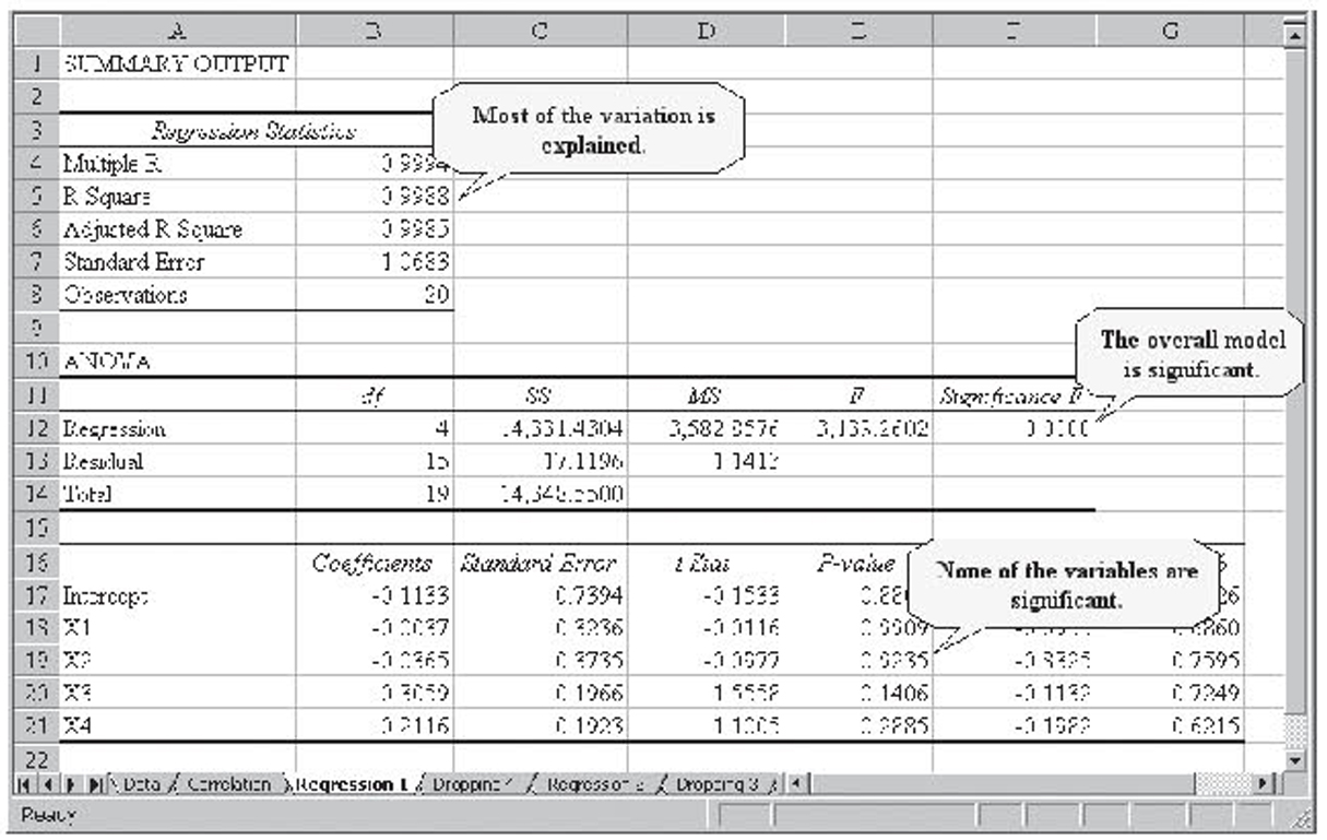
Figure 4.27 Initial regression run on the high-multicollinearity fictitious data
• The r2 value is 0.9988 so almost 100 percent of the variation in Y is being explained by the variation in the four independent variables. From this perspective, you could not ask for a better model.
• The overall model is significant. That is, it passes the F-test. This is to be expected given the high r2 value.
• None of the independent variables is significant. Here, we have an overall model that is significant yet none of the variables used to construct the model is significant. This is a very clear indicator of multicollinearity.
Normally, we would need to drop all four variables one at a time and record the resulting r2 values in order to decide which to drop. However, the way the data was constructed for this example guarantees about the same impact regardless of the variable dropped, so we will simply drop X4. The resulting multiple regression run is shown in Figure 4.28.
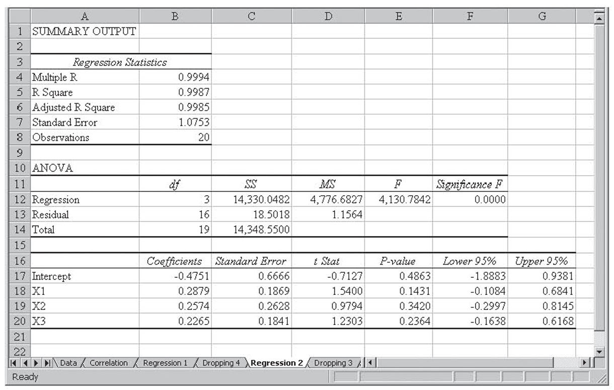
Figure 4.28 Regression run with the X4 variable dropped on the high-multicollinearity fictitious data
This time, notice the following:
• The r2 value does not change much, going from 0.9988 to 0.9987.
• The overall model is still significant.
• Again, none of the remaining independent variables is significant.
• The slope coefficients for X1 and X2 change dramatically, going from negative to positive. This will end up being one of the important signs of multicollinearity.
This time, we will drop X3. The resulting multiple regression run is shown in Figure 4.29. This time, notice the following:
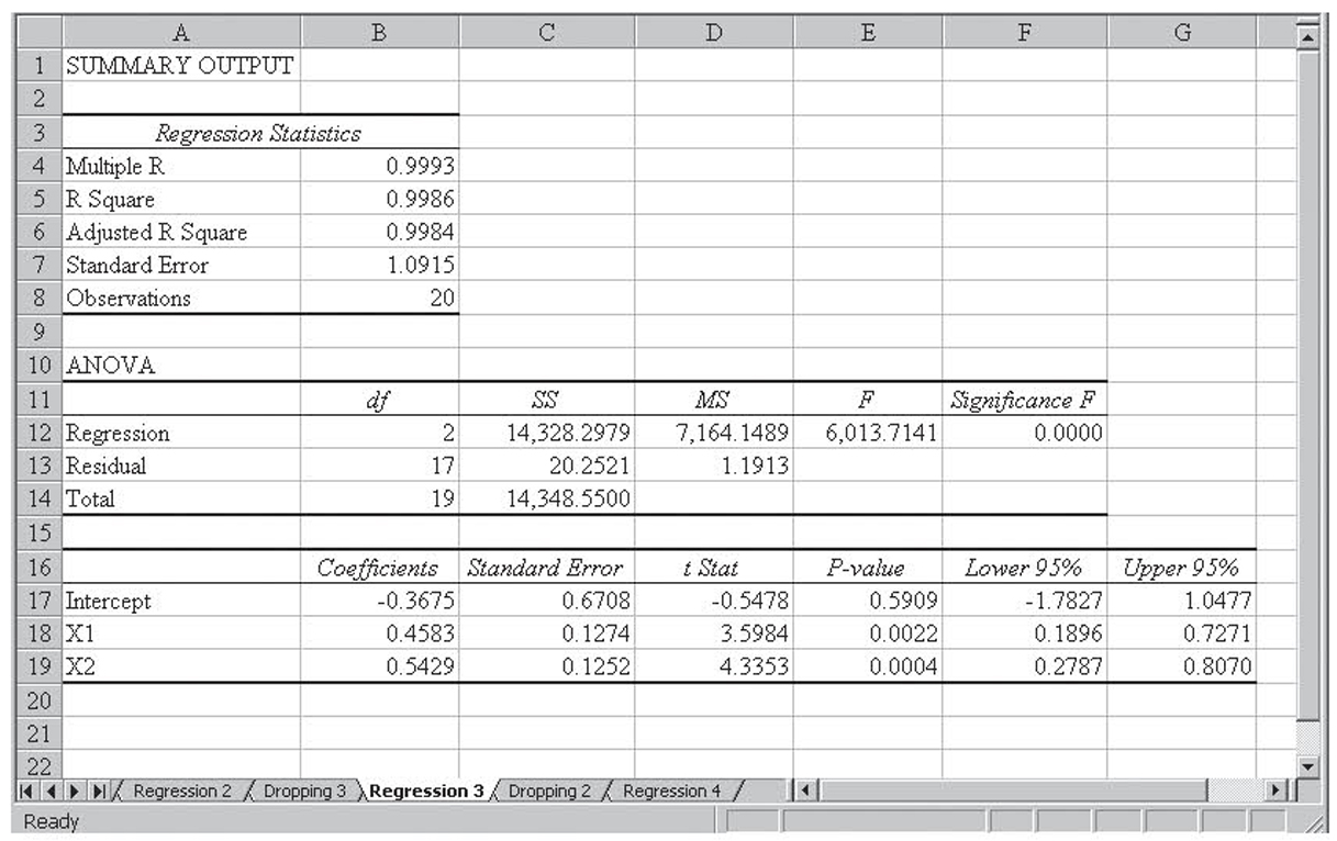
Figure 4.29 Regression run with the X3 and X4 variables dropped on the high-multicollinearity fictitious data
• The r2 value does not change much, going from 0.9987 to 0.9986.
• The overall model is still significant.
• This time, the two remaining slope coefficients are significant.
• Both of the remaining slope coefficients nearly double in magnitude.
Although this model meets all our criteria, we will go ahead and drop X2. The resulting simple regression run is shown in Figure 4.30. This time, notice the following:

Figure 4.30 Regression run with the X2, X3, and X4 variables dropped on the high-multicollinearity fictitious data
• The r2 value does not change much, going from 0.9986 to 0.9970.
• The overall model is still significant.
• The single remaining independent variable is significant.
Clearly, the model suffered serious problems relating to its high degree of multicollinearity, although the final model in Figure 4.30 no longer has a multicollinearity. Do you see why?
What Causes Multicollinearity?
Independent variables are selected based on their theoretical relationship with the dependent variable, not their statistical suitability for using in multiple regression. Oftentimes, a natural relationship exists between these variables.
For example, in the sales forecasting model we have been discussing, two of the variables we would naturally collect are levels of advertising and competitor actions, most likely in the form of competitor advertising. It is reasonable to assume that the higher our advertising spending, the more our competitors are going to spend on advertising. That is, when our advertising spending goes up, competitor spending is likely to go up, and when our spending goes down, competitor spending is likely to go down. In other words, these two independent variables are highly correlated, and therefore we have multicollinearity. That natural multicollinearity does not mean that we should not collect data on both variables. Remember, the decision on the independent variables to start with is a theoretical decision, not a statistical decision. Rather, it simply means that both variables may not make it to the final model or, if they do, the final model will have multicollinearity between these two variables. Researchers must understand this relationship if they are to interpret the results properly. After all, if competitor advertising does not make it into the final model, they need to understand why.
Flawed data-collection methods can also introduce multicollinearity into the model. For example, if sales data were only collected from stores with a high level of competition, the data set would show a stronger relationship between advertising spending and competitor spending on advertising than would be the case if all locations were included in the sample. That would introduce an unnaturally high level of multicollinearity between the two variables.
Spotting Multicollinearity
In the previous examples, we have already seen some of the ways in which multicollinearity can be spotted. In general, all of the following are indicators of multicollinearity:
The first indicator is a high correlation between independent variables in the correlation matrix. Unless they have been artificially created, as shown previously, all independent variables will have some correlation between them and this correlation will show up in the correlation matrix. A rule of thumb is that a value of 0.60 or higher in the correlation matrix is an indicator of multicollinearity strong enough to be concerned about. This is the easiest rule to use, so it is recommended that you produce a correlation matrix on each data set prior to running multiple regression. Because you want a high degree of correlation between each independent variable and the single dependent variable, you should only include the independent variables in this correlation matrix so the high values between the variables and the dependent variable does not confuse its interpretation.
The second indicator is a low tolerance. One drawback to testing for multicollinearity using correlations is that it only spots pairwise multicollinearity because it is based on pairwise correlation. It is possible to test to see there is multicollinearity between more than two variables; that is, if two or more independent variables combined together can explain another independent variable. To do this, you run multiple regression with one of the independent variables as the dependent variable and the remaining independent variables (not the dependent variable) as the independent variables. The tolerance is then computed as follows:
Tolerance
1 – r2
for this reduced multiple regression run. It is the case that the smaller the tolerance, the greater the multicollinearity regarding the independent variable being used as the dependent variable. The smallest possible value for tolerance is zero, and a good rule of thumb is that anything below 0.20 indicates a problem with multicollinearity. Two notes are in order. First, with k independent variables, there will be k measures of tolerance, as each independent variable is used, in turn, as the dependent variable. Second, tolerance requires at least three independent variables because with just two independent variables, the correlation coefficient is adequate for measuring multicollinearity. Finally, due to the difficulty of performing these repeated multiple regression runs, tolerance as a diagnostic for multicollinearity is not emphasized in this textbook.
The third indicator is important theoretical variables that are not significant. There are two main reasons why an important theoretical variable might not be significant: Either the theory is wrong or there is multicollinearity.8 If you are confident that the theory is correct, then the cause is most likely that another variable is robbing the theoretically important variable of its explanatory ability—in other words, multicollinearity.
The fourth indicator is coefficients that do not make sense theoretically. In the sales forecast example, the theory says that increasing advertising spending should increase sales, so we would expect a positive slope coefficient for advertising spending. If that does not happen, then either the theory is wrong or, once again, multicollinearity is causing another variable to rob the theoretically important variable of its explanatory ability and therefore, in the process, altering its coefficient.
Note that it is rarely possible to evaluate coefficients theoretically beyond their signs. This is because the magnitudes of the coefficients are determined by the units of the independent variable, the units of the dependent variable, and if multicollinearity is present, the units of the collinear variables. Change any of these units and the coefficient changes. That is, measure sales in thousands of dollars rather than dollars or advertising spending in minutes of television time instead of dollars and the advertising spending coefficient changes. However, regardless of the units, the sign of the slope coefficient should behave according to theory.
The fifth indicator is when you notice that dropping a variable causes dramatic shifts in the remaining coefficients. If there is no multicollinearity, then the explanatory power of a variable does not change as other variables come and go. We saw this in the previous example artificially created without multicollinearity. Therefore, when coefficients shift as other variables come and go, it is an indicator of multicollinearity. Thus we see that the greater the shift, the larger the multicollinearity. As discussed previously, the biggest concern is when the coefficients change signs or when values change by an order of magnitude.
The sixth indicator is when you notice that dropping a nonoutlier observation causes dramatic shifts in the coefficients. Although rarely used in practice, dropping a single observation that is not an outlier should not cause much of a shift in the coefficients. When it does, that is a sign of multicollinearity. Of course, this is also a sign that the observation is possibly an outlier so you must be careful in its use. One of the reasons this is not used much in practice is that it is the least likely of all the approaches to generate an observable effect, plus researchers rarely wish to drop useful data.
Treating Multicollinearity
When multicollinearity is present, any or all of the following can be used to treat it.
Fix the sampling plan. It goes without saying that when the multicollinearity was introduced by a poor approach to gathering the data, new data should be collected using a better sampling plan. It is much better to work with good data than it is to try to fix bad data.
Transform the collinear variables. Multicollinearity is a linear correlation between two (or more) variables. Transforming one or more of these variables in a nonlinear fashion can reduce or eliminate the multicollinearity. Nonlinear transformations include taking the log, squaring, and taking the square root. Multiplying by a number or adding a number are both linear transformations and will not change multicollinearity.
The trouble with transforming the data is that it changes the data. Changing the data makes it tougher to theoretically interpret the data. For example, we know that a positive slope coefficient for advertising indicates that spending more money on advertising increases sales. If sales and advertising are both measured in thousands of dollars, then a coefficient of 0.50 would indicate that for every additional thousand dollars spent on advertising, sales go up by $500. But what would the coefficient mean if we were using the log or square root of advertising dollars? For this reason, variable transformations are usually only used in models intended for prediction where there is little or no interest in understanding the underlying processes.
Transform the data set. An advanced statistical process called factor analysis can be used to transform a collinear data set, or any subset of that data set, into new, uncorrelated variables that explain the same variation as the original data set. However, these new and uncorrelated variables are even more manipulated than the simple variable transformations discussed previously, making them that much harder to theoretically interpret. Students interested in this topic should consult an advanced statistical textbook such as Philip Bobko’s Correlation and Regression: Principles and Applications for Industrial/Organizational Psychology and Management (1995, McGraw-Hill). Factor analysis was the technique used to create the completely uncorrelated variables used in an earlier example in this chapter.
Use an advanced multiple regression approach. A type of multiple regression called ridge regression is more adept at working with collinear data. Excel is not able to perform ridge regression.
Drop one of the collinear variables. After all, if the two variables are explaining the same, or mostly the same, variation, it makes little sense to include both in the model. When the multicollinearity between two variables is too high, it is rarely the case that both will end up being significant. Thus the model development procedures discussed previously will automatically cause one in the pair of collinear variables to be dropped. Even if they both end up being significant, they may end up biasing the coefficients to such an extent that one of them must be dropped so the remaining coefficients make theoretical sense.
Do nothing. If the collinear variables are all significant, then they help improve the fit of the model. If the model is to be used mainly for prediction, then any theoretical problems with the coefficients will not be a problem. Even when the model is to be used for understanding, multicollinearity does not always have such a strong impact as to cause the coefficients not to make theoretical sense.
One of the assumptions of regression, both simple and multiple, is that the error terms (ε) are independent of each other. Stated another way, εi is uncorrelated with εi–1 or εi–2 or εi–3 and so on. When correlation between one or more of these error terms exists, it is called autocorrelation.
Autocorrelation is only an issue when we have time-series data—that is, data that were measured at different points in time. For example, if we have quarterly measures of demand for several years, it is likely that the demand for any quarter was related to quarterly demand a year ago, so it is likely that εi is correlated with εi–4. This is called a lag four correlation.
This issue of lagged correlation can easily be illustrated with a figure. Figure 4.31 shows a one-period lag in the correlation of the error terms. This is called first-order autocorrelation. Figure 4.32 shows a two-period lag in the correlation. This is called second-order autocorrelation.
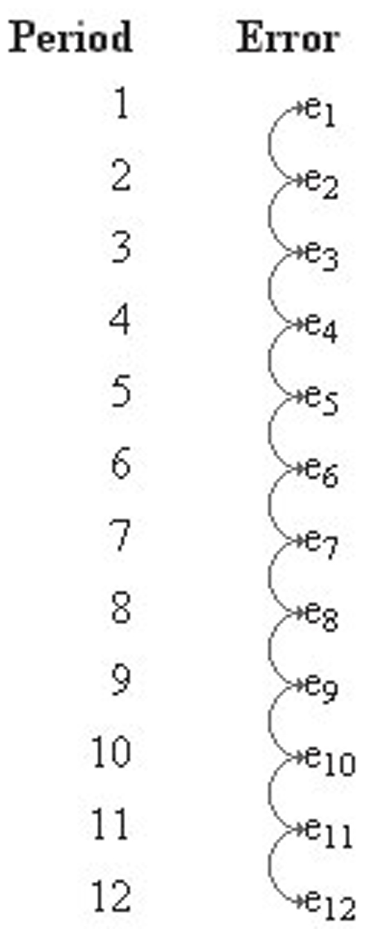
Figure 4.31 An illustration of lag one correlation
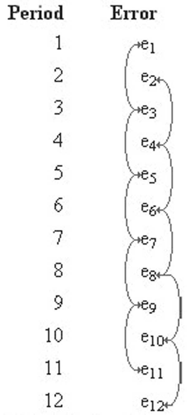
Figure 4.32 An illustration of lag two correlation
When the data are not time series, there is no reason to be concerned about autocorrelation. After all, there is not likely to be any relationship between the different dependent variable observations, so there is unlikely to be any correlation of the error terms. Although it is technically possible for the error terms to be correlated for non-time- series data (called cross sectional data), we need not be concerned with this rare occurrence. After all, if the data are not time-series data, there is no specific order for the data. Therefore, we could simply rearrange the sequence of the data and alter any lag correlations of the error terms.
Statistical software, like SPSS or SAS, can compute a Durbin-Watson test to easily spot first-order autocorrelation. The hypotheses for the Durbin-Watson test are the following:
H0 : ρ1 = 0
H0 : ρ1 ≠ 0
Of course, we can also perform a one-tailed version of the test. The hypotheses use a ρ1 because the Durbin-Watson test can only spot first-order autocorrelation.
The calculated Durbin-Watson statistic value can take on values between zero and four. A value of two, which is in the middle of this range, indicates no autocorrelation. A value of zero indicates positive autocorrelation and a value of four indicates negative autocorrelation. When a table is not available, a rule of thumb is that values of d between 1.5 and 2.5 indicates no autocorrelation. The Durbin-Watson test statistic d is defined with the following equation:
Durbin-Watson Test Statistics

A couple of notes are in order regarding this formula. First, notice that although we are testing for the significance of a correlation, neither a sample (r) or assumed population (ρ) correlation coefficient is used in the calculations. Second, note that the top of the formula is summed from “i = 2 to n” whereas the bottom is summed from “i = 1 to n.” This is because the top measures the lagged squares and e1 – e0 is not defined.
The Durbin-Watson test first appears to work differently than the other hypothesis tests we have looked at. For a one-tailed test,9 the critical values (dL and dU)10 do not divide the distribution into acceptance and rejection regions. Rather, they divide the distribution into five different regions, as noted in Table 4.1.
Table 4.1 Durbin-Watson Outcome Regions

The lack of clear boundaries between the acceptance and rejection regions is, in fact, not due to the Durbin-Watson test working differently than other hypothesis tests. Rather, the actual boundaries of the test depend on the regression coefficients. Because printed tables cannot easily reflect this, the ranges where the test is inconclusive represent the range of possible values from the table for different values of the regression coefficients.
Example
It is very common for businesses to collect data, such as sales data, over time. Because these data are collected over time, it often has autocorrelation. We will explore this issue with an example.
Figure 4.33 shows sales data for 20 periods, along with the advertising and promotion data for the same period that will be used to explain the sales. That is, Sales is the dependent variable and Advertising and Promotion are the independent variables. This figure shows the data in Excel, and it is saved in Durbin-WatsonExample.xls if you wish to experiment with the data; however, the regression analysis will be performed using SPSS.
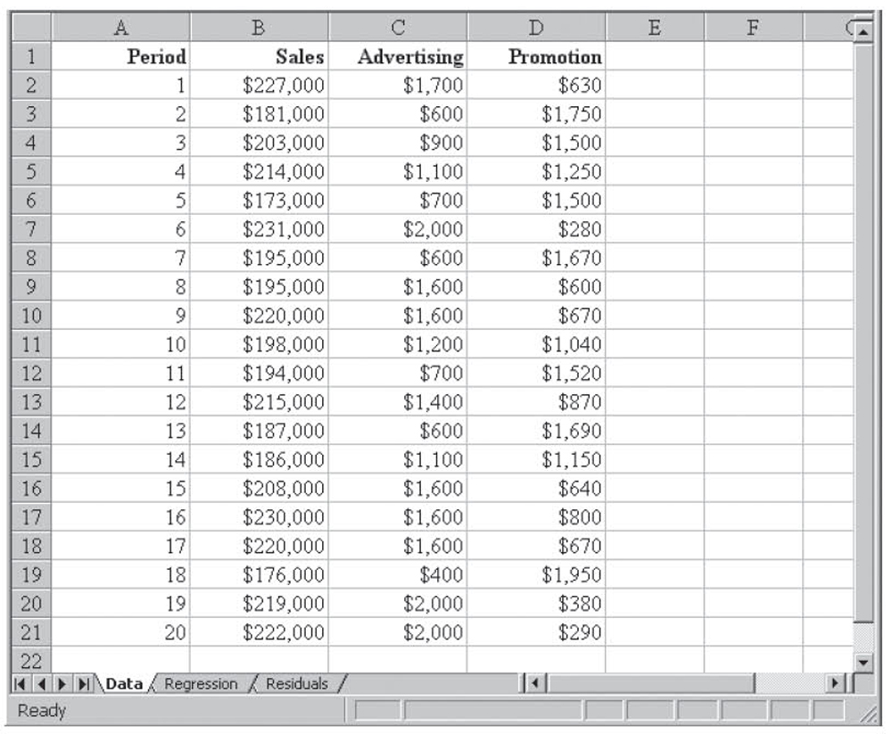
Figure 4.33 Data for Durbin-Watson example in Excel
Figure 4.34 shows the resulting multiple regression run. Note that the overall model is significant, and both of the independent variables are significant. This model explains 79.1 percent of the variation in sales.
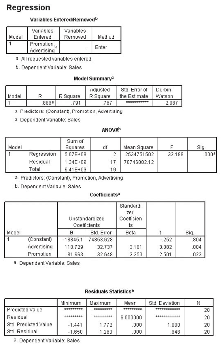
Figure 4.34 The results of running multiple regression using SPSS
The value of d from the model summary area is 2.087. Because we do assume that the autocorrelation is either positive or negative and d is between 1.5 and 2.5, we use a two-tailed test and conclude that there is no autocorrelation.
The value of d can be approximated using the following formula:
Approximating Durbin-Watson d
2(1 – r)
where r is the correlation coefficient that measures the association between successive residuals.
Although not shown, the regression model for the Durbin-Watson example was computed in Excel and the residuals were saved. The Residuals tab of the Durbin-WatsonExample.xls worksheet computes the correlation coefficient between successive residuals. That value is –0.06491. Applying the approximation formula above, we have 2[1 – (–0.06491)], which equals 2(1 + 0.06491), which is about 2.12983. That is close to the 2.0869 calculated by SPSS.
Treating Autocorrelation
There are two things you can do to minimize the possibility of having autocorrelation when dealing with time-series data. The first is to transform the data. When variables are measured in dollars over time, state those dollars in a constant unit, such as discounted dollars. When the dollars are left in their raw form,11 changes in the buying power of the dollar over time are built into the dependent variable but will not be accounted for by any independent variable. Furthermore, those changes over time are fairly regular and therefore correlated with one another, leading to autocorrelation. Converting to discounted dollars removes this time-based source of variation. In business, this is by far the most common transformation. Another transformation that works well, especially with economic and financial data, is to restate the variables as a percentage change.
When one or more independent variables are measured in their raw form, they have a built-in variation that is not being used to explain the dependent variable. As a result, this variation is transferred to the error term, where it becomes autocorrelation. Converting the variables to discounted dollars or percentage change removes this source of variation.
The second approach is to add a new independent variable, here called Period, where Period is simply a measure of the changes over time. This variable will explain this regular variation and keep it from reaching the error term. If Period is significant, then autocorrelation exists and Period treated it. If Period is not significant, then autocorrelation is not present.
The period variable should be a linear variable when every one-unit change in periods causes the same change in the period variable. The most common approach is to label the first period 1, the second 2, and so on. With annual data, using the actual year number would also work. For quarterly data, you could use sequential period numbers or year numbers with a.00, .25, .50, and .75 added for the different periods within each year.
You must be careful in labeling your periods. It is often tempting to use a labeling scheme that violates the assumption of equal units between the periods. For example, none of the following methods is appropriate:
• With monthly data, using 2002.01, 2002.02, . . . ,2002.11, 2002.12, 1991.01, and so on
• With quarterly data, using 2002.1, 2002.2, 2002.3, 2002.4, 2003.1, and so on
• With quarterly data, using 1, 2, 3, 4, 1, 2, 3, 4, and so on
With each of these, the gap between some sequential pairs of periods is different from other sequential pairs, and this nonlinear ordering of the periods violates the linearity assumption of regression.
Second Durbin-Watson Example
Figure 4.35 shows a set of data especially constructed to contain positive autocorrelation. The data are stored in the Excel file DW-2.xls for easy manipulation. Figure 4.36 shows the initial multiple regression run on this data. Note that the overall model is significant and both independent variables are also significant. However, the model only explains 53.1 percent of the variation in sales. This model has positive autocorrelation, as shown by the Durbin-Watson statistic of 0.101 shown in Figure 4.36.
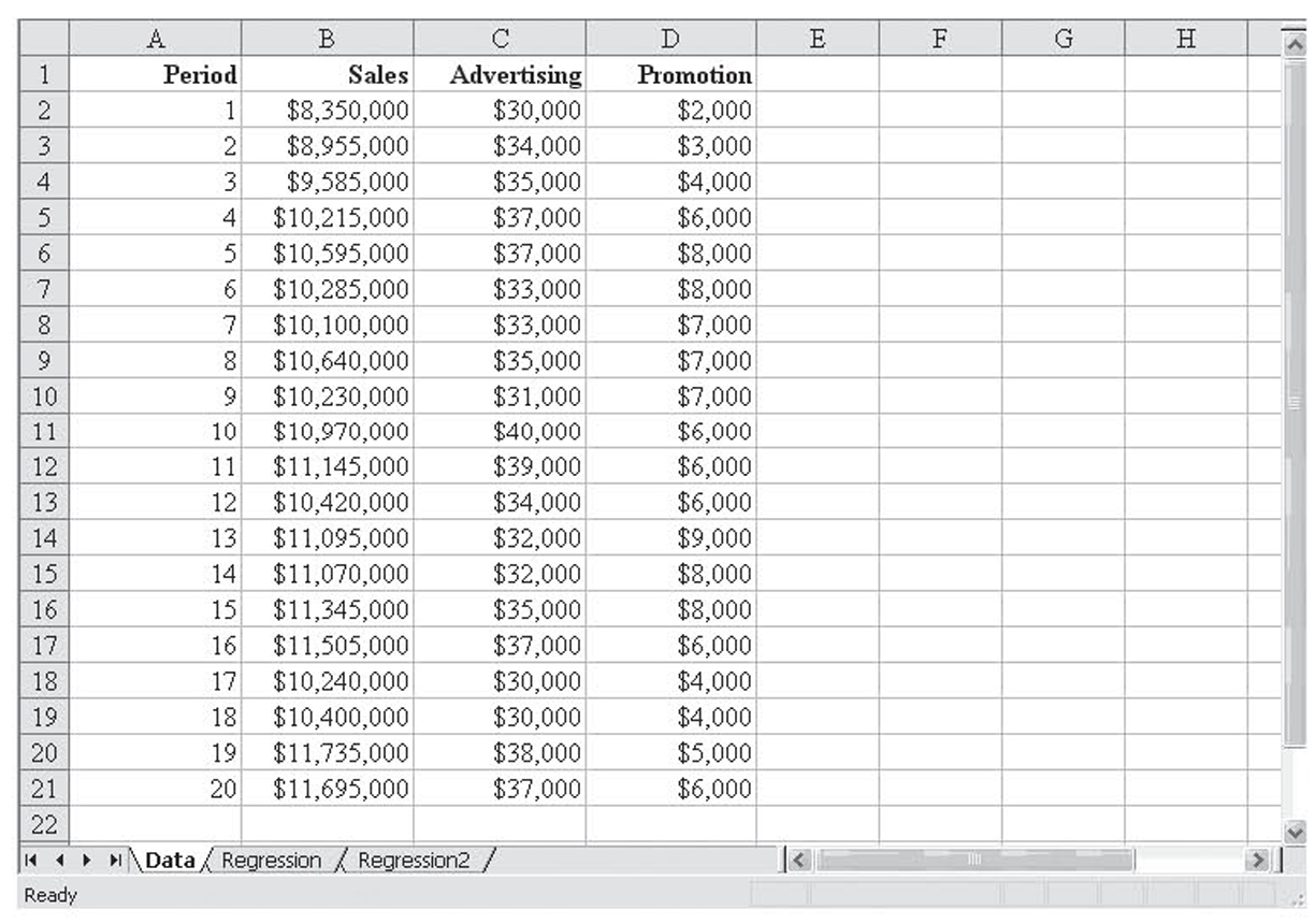
Figure 4.35 Data especially constructed to contain positive autocorrelation
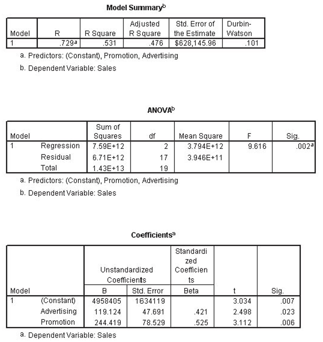
Figure 4.36 Initial regression on this fictitious data
To correct the autocorrelation, the period variable is added to the model as a third independent variable. That regression run is shown in Figure 4.37. Again, the overall model is significant and all three independent variables are significant. The explanatory power of the model goes up from 53.1 percent to 98.7 percent. This model has much less autocorrelation, as shown by the Durbin-Watson statistic of 2.836 shown in Figure 4.37.

Figure 4.37 Redoing the regression model by adding period as a variable
Heteroscedasticity
One of the assumptions of regression is that the error terms have equal variance. We called this homoscedasticity. Violating the assumption of homoscedasticity is called heteroscedasticity.12 Although heteroscedasticity is a violation of the assumptions of regression, it is a fairly minor violation relative to multicollinearity and autocorrelation. However, when heteroscedasticity is high, the researcher may need to build a separate regression model for each range of the error term. That is, the researchers need to build one model for the range where the variance is high and another for where it is low.
We will not be using a hypothesis test approach to testing for heteroscedasticity; rather, we will be using a visual approach. Specifically, we will be looking at a plot of the residuals (error terms) once the model has been built. Residuals are shown on the Y-axis. We must produce a plot for each independent variable that makes it into the final model. Fortunately, Excel makes this easy.
As we saw earlier, our Celebrities.xls worksheet has six independent variables and all of them are significant except for Earnings. We will now drop Earnings, produce the final model, and get a plot of the residuals. To add the plots to the output, we simply check Residual Plots in the Regression dialog box. Excel produces the plots and stacks them on top of each other, as shown in Figure 4.38. You click on the plot you wish to see and that brings it to the front. Figures 4.39 through 4.42 show the individual plots.
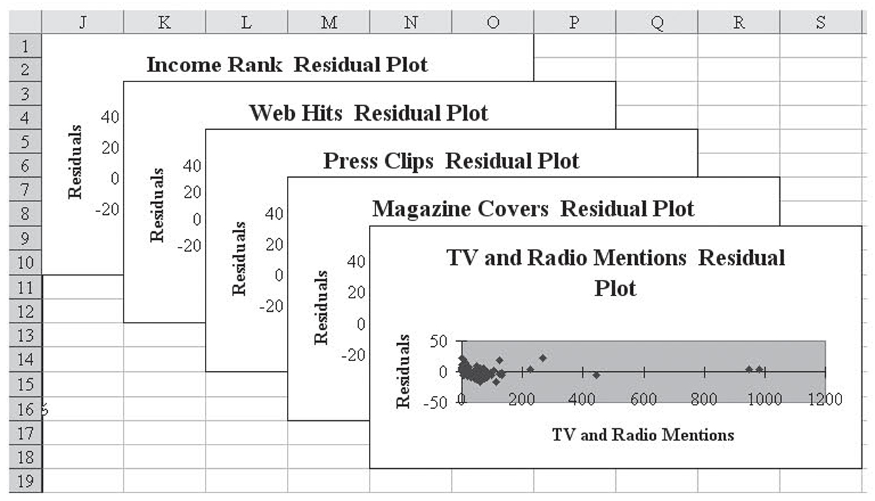
Figure 4.38 The stacked plot of residuals
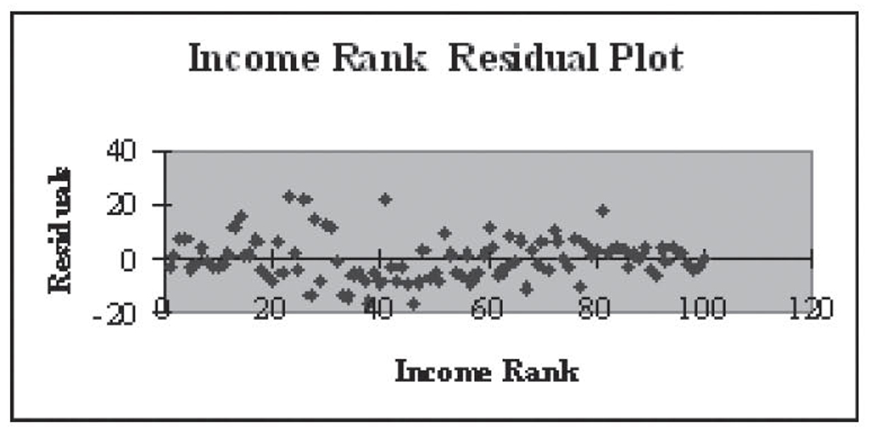
Figure 4.39 Residuals plotted against Income Rank
Figure 4.39 shows Residuals plotted against Income Rank. As Income Rank increases, the residuals appear to be randomly distributed when fairly consistent variability, so heteroscedasticity is not an issue. Figure 4.40 shows Residuals plotted against Web Hits. Clearly, the residuals are neither randomly distributed nor have equal variability, a clear sign of heteroscedasticity. Figure 4.41 shows Residuals plotted against Press Clippings. As with Figure 4.40, heteroscedasticity is clearly evident.
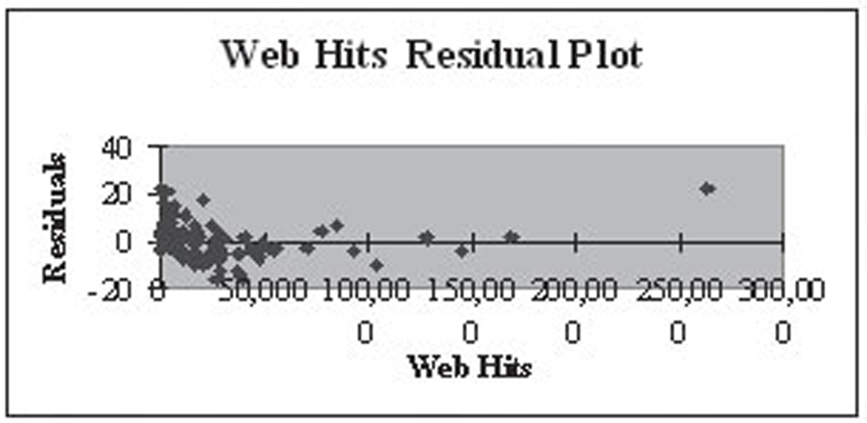
Figure 4.40 Residuals plotted against Web Hits
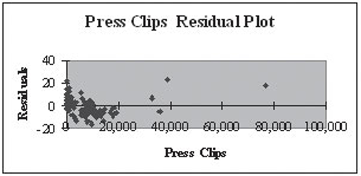
Figure 4.41 Residuals plotted against Press Clippings
Figure 4.42 shows Residuals plotted against Magazine Covers. With this variable, it is much harder to visually gauge heteroscedasticity. Magazine Covers can take only a limited number of discrete values and so the residual values are bunched above these few values. Dummy variables have this problem as well as discrete variables, only with dummy variables, there are only two columns of points. Although the variability clearly declines as the number of Magazine Covers decreases, this may be due more to the lower number of observations than to a decline in the variance. Therefore, the best we can say regarding heteroscedasticity is that we are uncertain.
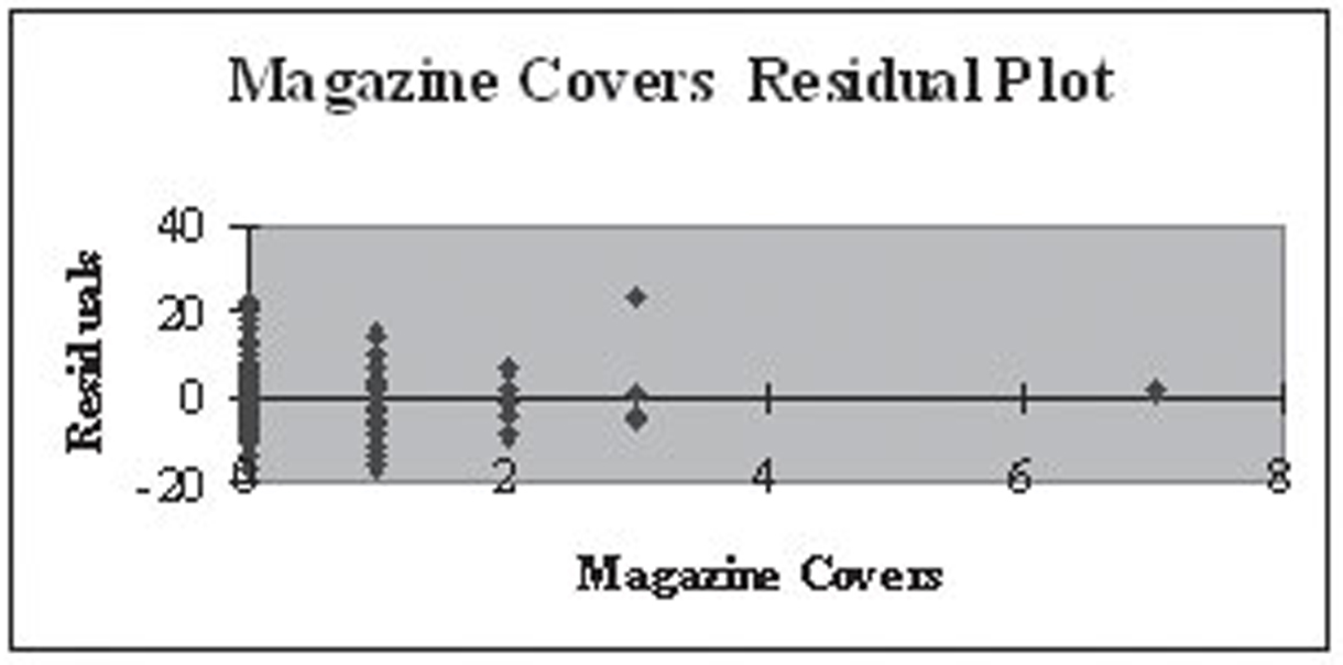
Figure 4.42 Residuals plotted against Magazine Covers
Figure 4.43 shows Residuals plotted against TV and Radio Mentions. The values on the left side of the chart appear to be randomly distributed with fairly constant variability. The very few observations on the right clearly have less variability but there are too few values to make any real judgment. These could simply be outliers. The most reasonable conclusion is that the bulk of the data shows no heteroscedasticity.
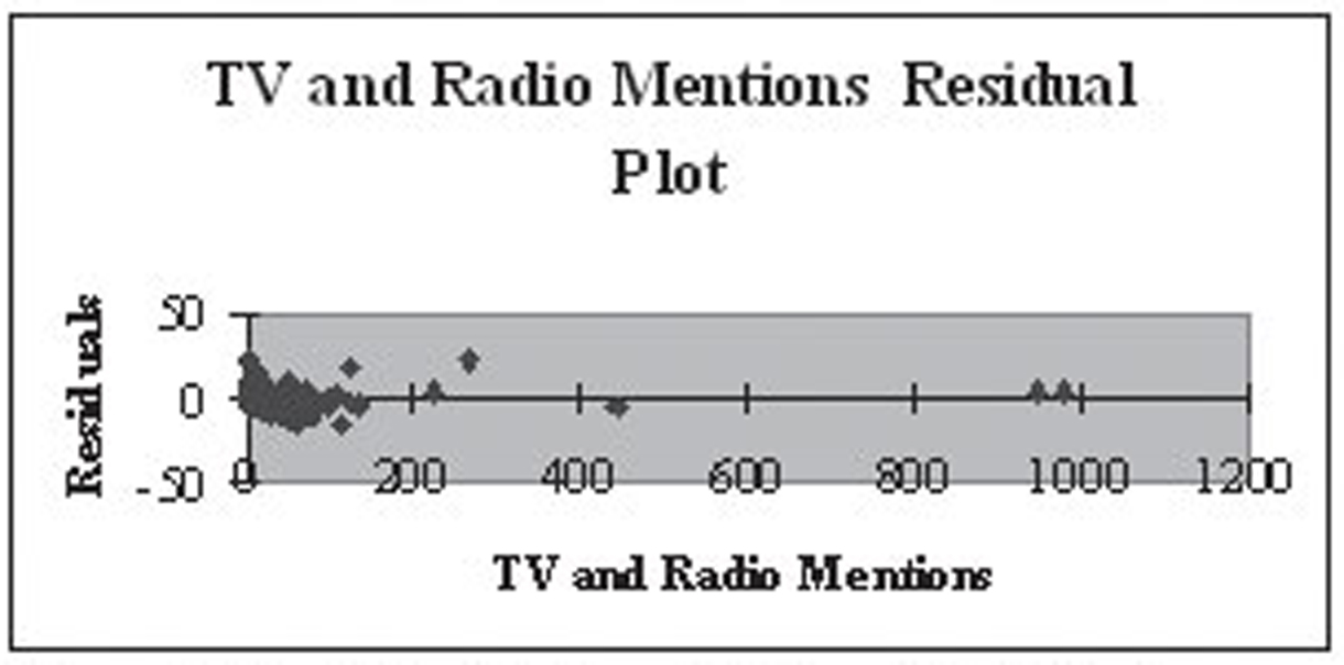
Figure 4.43 Residuals plotted against TV and Radio Mentions
The problem with gauging heteroscedasticity from these individual plots is that they do not show the error terms relative to all the data at once. It may be that large differences relative to one variable may not be too large when other variables are included in the comparison. The way to gauge heteroscedasticity across all the variables at once is to use a chart that Excel does not automatically compute—a plot of the standardized residuals against estimated values of the dependent variable. A homoscedastic model will display a cloud of dots with no visible pattern, whereas heteroscedasticity will be characterized by a pattern, such as a funnel shape, indicating greater error as the dependent increases.
Using the Celebrities.xls worksheet discussed previously, multiple regression was rerun, using SPSS and requesting a plot of the residuals. This is shown in Figure 4.44. The Y-axis is the standardized residuals and the X-axis is the standardized predicted values. With homoscedasticity, you would expect the spread of the data to be fairly consistent as you move from left to right. Because this data has a fairly narrow spread on both ends with a wider spread in the middle, it is an indication of heteroscedasticity. This measure looks at all the variables at once. This plot can be produced in Excel by having regression save the residuals, manually build a formula to calculate the predicted values, and then manually produce the plot. This exercise is left for interested readers.
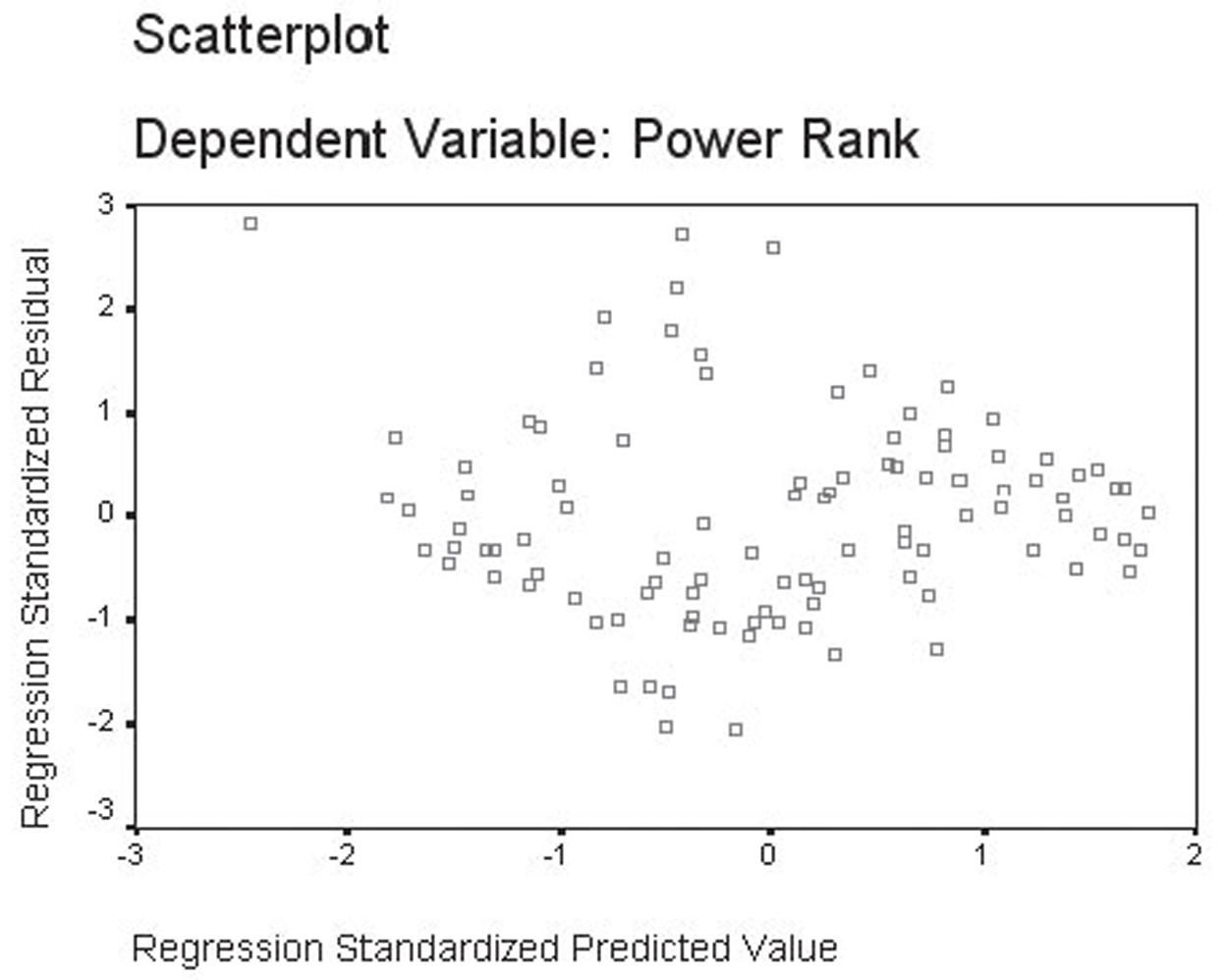
Figure 4.44 Plot of the residuals against predicted Y-values
Heteroscedasticity is a violation of the assumptions of regression; however, its effect is much smaller than either multicollinearity or autocorrelation. Heteroscedasticity causes the least squares estimation method to be less efficient. One approach to dealing with heteroscedasticity is to use weighted least squares. Excel is not able to perform this, so we will not explore it further.
A second approach is to transform the variable exhibiting heteroscedasticity using a nonlinear transformation such as squares, square roots, or logs. These transformations are particularly effective when the data show high variability on one side of the residual plot and low variability on the other. However, a nonlinear transformation introduces all the theoretical interpretation concerns raised earlier.
A third approach is to simply realize that heteroscedasticity exists in the multiple regression model but to otherwise ignore it in the calculation of the model. Given the minor impact of heteroscedasticity, this is the approach often taken by researchers.
Summary
In this chapter we looked at model building, incorporating qualitative data, and testing the validity of the model. You should now be ready to build your own multiple regression models.