The Data Vault layer is loaded from the data in the staging area. This chapter describes loading techniques using SSIS and T-SQL for loading hubs, links, and satellites, as well as advanced tables. It is fairly simple to transfer these concepts from Microsoft SQL Server to other BI toolkits. The chapter also discusses how to (soft) delete data from hubs and links and how to deal with missing data. It also covers how to load reference tables and ends with a discussion about truncating the staging area, which completes the loading process. The authors provide some modifications of the standard templates that are helpful when dealing with large amounts of data.
Keywords
staging area
loading techniques
SSIS
T-SQL
hubs
links
satellites
advanced tables
templates
This chapter focuses on the loading templates for the Raw Data Vault. These templates are built on some basic rules and best practices that have been accumulated over multiple years of experience. The patterns have evolved because of multiple performance issues with legacy ETL code. The top issues that affect the performance of the ETL loads are:
1.Complexity: the performance is affected by the variety of the data structures that need to be loaded into the data warehouse, but also by the data type alignment and the conformance of the data to set definitions. This is becoming a significant problem when dealing with highly unstructured data where the data structure changes from one record (or document) to the next.
2.Data size: volume also plays an important role regarding data warehouse loads. The more data is loaded, the more exposed are performance problems in the loading architecture and design.
3.Latency: the velocity of the data sources influences the frequency of the incoming data. If data needs to be loaded with high frequencies, small problems in the data flow will be exaggerated, leading to many more issues than before. Fast-arriving data also prohibits complexity in the processing stream because, depending on the infrastructure used, data might be lost if processing takes too long.
The complexity of the loading patterns is often additionally influenced by business rules that need to be processed upstream of the data warehouse. While the intention is to reduce the complexity of the data, the actual effect is that these business rules make the processes more complex because they change. The effect of the changed business rule has to be taken into consideration in later stages, which represents the majority of the increase in complexity.
When analyzing the fundamental issue of the ETL performance in many data warehouse projects, findings based on set logic (shown in Figure 12.1) are important to understand.
Figure 12.1Set logic for data warehouses.
When dealing with a specific number of records that are loaded into the staging area, only about 60 to 80% are inserted records that have never been seen by the data warehouse before; 10 to 20% are updates of descriptive data to keys that are already in the data warehouse. And 5% of the incoming data describe deletes in the source system that should be tracked by the data warehouse as soft-deletes.
If only 20% of, e.g., 10 million rows (that is, 2 million rows) were identified by key, to be updates, then the aggregations of those 2 million rows would be even less – especially by month, quarter, and year. Those updates will identify specific sets of denormalized keys to be updated, along with a specific point in time. It would then be easy to meet performance objectives in a well-tuned relational database management system (RDBMS) environment.
However, many data warehouse developers construct their ETL routines to deal with the whole dataset in staging. If the problem were separated, each resulting individual process would have to deal with a decreasing process complexity, which makes it possible to increase performance, as we will learn a little later.
The key to improving the performance of data warehouse loading processes is based on two ideas:
1.Divide and conquer the problem: separate the processing of the loading procedures into separate groups in order to deal with smaller problems using a focused approach. In data warehousing, there are two different goals that should be reached individually: data warehousing and information processing.
2.Apply set logic: reduce the amount of data each process deals with by separating the data into different processes and reducing the amount of data as it is being processed.
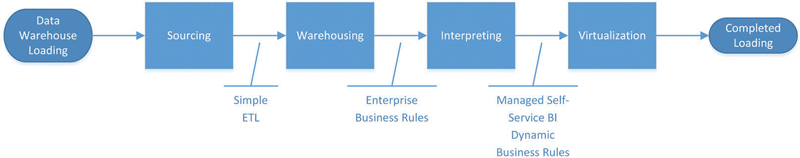
The first idea is depicted in Figure 12.2: the two major goals are further divided into two separate activities each.
Figure 12.2Overall loading process of the data warehouse.
Data warehousing is different from sourcing of data because it has different issues:
•Latency issues: the performance of subsequent processes is affected by the latency of the source. Because the latency of the actual source system is not stable and varies over time, the staging area is used during sourcing to provide a stable latency of the incoming data. In other cases, data arrives in real-time which has to be taken into consideration by the sourcing application as well.
•Arrival issues: not all data arrives at the same time. The staging area is used to buffer the incoming data and makes sure that all dependencies are met if actually required.
•Network issues: the network could be the source of errors as well, for example when the network connection is too slow or important network devices or servers are unavailable.
•Security issues: in other cases, the data warehouse doesn’t have access to the source system because the password was changed or expired.
This is the reason why the data is “dumped” into the staging area in order to separate these problems from the actual data warehousing. Each activity in Figure 12.2 deals with a separate problem. Some of these problems are also neutralized by using a NoSQL environment such as Hadoop or a similar technology.
In order to ensure the performance of the loading processes, the following rules should be followed:
1.Decrease process complexity: simplicity beats complexity. Simple loading processes are not only easier to maintain and administrate, they are also superior regarding performance.
2.Decrease the amount of data: reduce the amount of data that needs to be touched in order to load the target. This can also be achieved by using parallel processes where each process or thread is dealing with a smaller amount of data than the unparallelized process.
3.Increase process parallelism: the server is able to process multiple execution paths at the same time. For this reason, the intraoperation (inside one process) and interoperational (multiple processes) parallelism should be increased to take advantage of these capabilities.
4.Combine all three: to achieve superior performance, combine all three rules by reducing the complexity of the loading processes, decreasing the amount of data, and increasing the process parallelism, all at the same time. The best way to achieve this goal is to tackle one rule at a time.
Note that parallelism is last on the list, and should be avoided as long as possible, because any time a process is partitioned or parallelism is added, maintenance costs are increased. Instead, data warehouse teams should focus first on decreasing the complexity of the loading processes, yet many organizations don’t even deal with this first rule. Also note that the parallelization requires that referential integrity be turned off in the Raw Data Vault, at least during load.
The overall loading process of the data warehouse implements these recommendations (Figure 12.3).
Figure 12.3High-performance processes for the data warehouse.
Each phase of the loading process deals with a separate problem. By doing so, each phase also deals with progressively less data. Data is only loaded into the enterprise data warehouse (EDW) layer if it is new and unknown to the layer. And only data that is required for incrementally building the information mart is pushed into the next layer. This is also due to the fact that set logic has been applied to further reduce the amount of data to be dealt with. The separation of loading processes also favors highly simplified and focused loading patterns because each layer has a specific focus that is reflected in the loading patterns. The time each simplified phase requires is short due to high parallelization. Because of this short required time-frame, the overall process is short as well.
However, parallelization is not limited to one source system. The goal of the data warehouse loading processes is to load source systems as soon as they are ready to be loaded into the data warehouse. Waiting until a specific time in the night when all source systems are ready to be loaded into the data warehouse should be avoided. Instead, once a source system has provided its data to the data warehouse, it is staged, loaded to the data warehouse and, if possible, all information marts that directly depend on this data are processed. Figure 12.4 depicts this staggered approach.
Figure 12.4Staggering the load process of multiple source systems.
In the figure, the data from multiple source systems is provided to the data warehouse at different times. Once the data is available to the data warehouse, it is staged immediately. It is also possible to load the data into the Raw Data Vault because there are no dependencies that require any waiting. In the case of Figure 12.4, all information marts depend on only one data source, which is a simplified example. In reality, there are synchronization points that have to be taken care of.
However, some of the dimension and fact tables that only depend on the one source system or have all other dependencies met (all other source systems loaded already) can be processed. This approach helps to take advantage of the available data warehouse infrastructure and increases the load window of the data warehouse because the peak in the loading process is reduced. It disperses the load of the engine over time and makes it possible to increase the number of loads for some of the source systems. Instead of loading the data only once a day, the data can be sourced multiple times a day because the loading processes are independent from each other and computing power remains available. Loading the data from a single source system multiple times a day also has the advantage that each single run can deal with less data if delta loading is used. However, it also requires that the data warehouse meet more operational requirements, such as a better uptime and more resiliency and elasticity of the data warehouse infrastructure.
This chapter presents the recommended templates for loading patterns of many Data Vault 2.0 entities. These templates are based on experience and optimization from projects and take full advantage of the Data Vault 2.0 model and the rules and recommendations outlined earlier in this chapter. Examples in T-SQL and SSIS are also provided for each presented template. It is easy to adapt the examples to ANSI SQL or other ETL engines.
12.1. Loading Raw Data Vault Entities
Similar to the staging area, the enterprise data warehouse layer has to be materialized. This EDW layer is responsible for storing the single version of the facts, at any given time. Therefore, virtualization is not an option for most entities in the EDW layer (some exceptions are discussed in section 12.2.1) and the Business Vault, which is discussed in Chapter 14, Loading the Dimensional Information Mart.
Implementing the loading processes for the Raw Data Vault only requires simple SQL statements, such as INSERT INTO <target> SELECT FROM <source> statements. However, organizations often prefer to implement loading processes in ETL to more easily offload the required processing power to their existing ETL infrastructure, leveraging their ETL investments. For this reason, both options using SSIS and T-SQL are demonstrated in the next sections: each section focuses on one target entity, such as hubs, links, and satellites, including their special cases. The goal of the Raw Data Vault is to store raw data, so all patterns move raw data only. The data is extracted from the staging table and loaded into the target entity in the Raw Data Vault without modifications.
Note that the loading patterns use the load date from the staging area. However, it is also possible to create a new load date within the loading processes (for example, using GETDATE() or a similar function). The key is to control the load date within the data warehouse and not rely on a third-party system such as an operational source application.
The performance of the loading patterns is not only due to the design principles for data warehouse loading, as outlined in the previous section. It is also due to the use of hash keys instead of sequence numbers. The hash keys are used to overcome lookups into parent tables, which hinder parallelization and reduce performance due to higher I/O requirements. The characteristics of using hash keys in data warehousing have been discussed in the Chapter 11, Data Extraction. The loading templates presented in this chapter take direct advantage of these characteristics.
12.1.1. Hubs
When loading data from the staging area into the enterprise data warehouse layer, the Data Vault hubs are supposed to store the business keys of the source systems. This list has to be updated only in a single regard: in each load cycle new keys that have been added to the source system are added to the target hub. If keys get deleted in the source system, they remain in the target hub. The template for loading hub tables is presented in Figure 12.5.
Figure 12.5Template for loading hub tables.
The first step is to retrieve all business keys from the source. This step is not as trivial as it sounds. In many cases, there are multiple source tables within one source system that provide the same business keys because they are shared across the system. For example, a passenger table provides a list of passenger identification numbers and a table holding ticket information references the passenger using its business key (see Figure 12.6).
Figure 12.6Combining business keys from multiple sources.
In order to guarantee that all passenger identification numbers have been sourced to the target hub table HubPassenger, the keys from all source tables have to be sourced using a UNION operation, as shown in this figure, or by running the template in Figure 12.5 multiple times, for each source table. In many cases, the second approach is the most favorable because it makes automation of the loading processes more feasible, for example by allowing a metadata driven definition of the loading patterns (refer to Chapter 10, Metadata Management, for more details).
In both cases, the question becomes which record source is set in the target hub table. The record source in the target reflects the detailed source system table that has provided the business key to the data warehouse for the first time. If multiple tables (or even multiple source systems) provide the business key at the same time, a predefined master system table is set as the record source. This master system table is usually identified in the metadata and has the highest priority. If multiple patterns are used to load the same target hub table, the source table with the highest priority (as defined in the metadata) is sourced first. This way, the key found in the source tables with the highest priority will set the record source, because the duplicates in other sources will not be sourced anymore.
This behavior is guaranteed by the second step in Figure 12.5, which checks if the business key already exists in the target. This is done by performing a lookup into the target table to find out if the business key from the source already exists. Only new keys are processed further. Because this lookup should be performed only once per business key, only a distinct list of business keys were sourced from the source table in the staging area in the first step. This follows the approach of reducing the amount of data processed by the data flow as soon as possible.
Because the staging area contains both the business key and the hash key, both keys are sourced from the staging table and become available in the data flow. The lookup is performed using the business key and not the hash key. This is because of the rare risk of hash collisions described in the previous chapter. If two business keys produce the same hash key, a lookup on the hash key would return that the hash key already exists in the target. But due to the hash collision, this would mean a different business key. Performing the lookup on the business key will return a hit only if the business key already exists in the target table, regardless of the hash key. However, in the case of a hash collision, this will result in a primary key constraint violation when inserting the record in the next step. This is not the preferred solution, but it is the desired one, because we’d like to be notified in case of collision. Despite the low risk of a hash collision, the impact is high: if a collision happens, the hash function should be upgraded as described in Chapter 11, Data Extraction.
If a business key already exists in the target, the record is dropped from the data flow. Only if the business key doesn’t exist in the target hub table, it is inserted into the target table. As already stated, the hash key is not calculated in this process because it is sourced from the staging table. If the business key consists of multiple parts, a so-called composite key, the process remains the same. The only difference is that the lookup has to include the whole composite key when performing the lookup operation.
Because the hub table stores all business keys that have been in the source systems in any point of time, this process doesn’t delete any business keys or updates them for any reason. Once a business key has been inserted to the hub table, it remains there forever (not quite true if data has to be destructed for legal or other reasons).
12.1.1.1. T-SQL Example
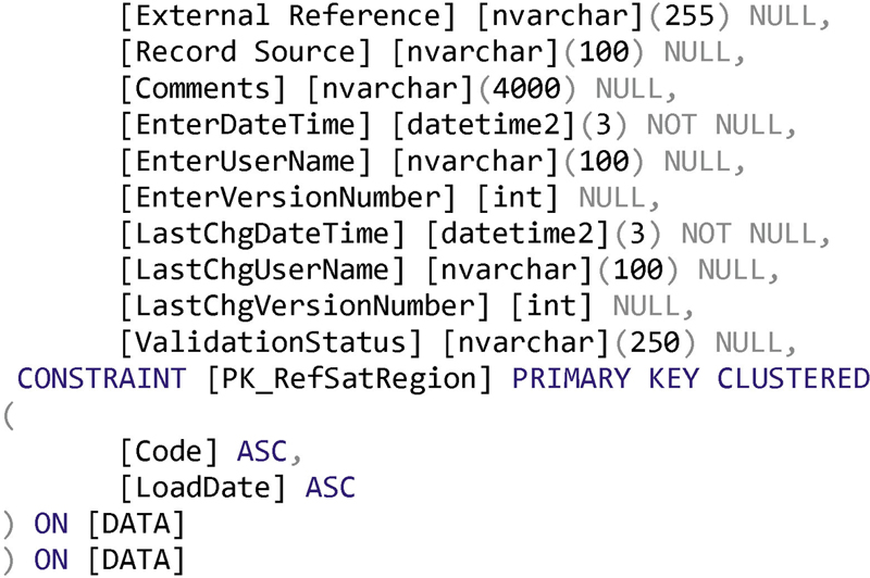
The following DDL creates a target hub for the airport code found in the BTS performance data:
Throughout this book, the raw schema is used to store the tables and other database objects of the Raw Data Vault. The hub contains a hash key, which is based on the airport code columns from the source. In addition, it contains a load date and a record source column. The defining column is the AirportCode column at the end of the table definition. The use of a nonclustered primary key is strongly recommended because the hash key is used as the primary key. Because the hash key has a random distribution, the keys will not arrive in any order. If a clustered primary key were used, Microsoft SQL Server would rearrange the data rows on disk whenever a new record arrived. This would slow down INSERT performance and provide no value to the retrieval of data from the table. Therefore, we always use nonclustered primary keys, except for very small tables with a small number of inserts. In addition to the primary key on the hash key column, an alternate key is added in order to speed up lookups on the business key.
In order to load newly arrived airport codes from the source table in the staging area, the following T-simplified SQL command can be used:
Note that if the hub is defined by a composite business key, the NOT IN statement might not work, depending on the selected database management system. Microsoft SQL Server only supports one column in a NOT IN condition. However, it is possible to use a NOT EXISTS condition to overcome this limitation. This is done in the link loading statement in section 12.1.2.
The diversion airports are NULL if no flight diversion happened. This special case might be wrong from a business perspective, but nonetheless the NULL business key is also sourced into the hub because some links and satellites might use it as well (for example, see the link loading process in section 12.1.2).
Only keys which are unknown to the target hub should be inserted to avoid errors: if duplicate business keys or hash keys are inserted into the hub table, either the table’s primary key on the hash key column or the alternate key on the business key column will raise a duplicate value error. To avoid the error, the first check in the WHERE clause is to check whether the business key is already in the target hub. This approach is the safest, because it detects hash collisions (refer to Chapter 11). But it also requires an index on the business key for faster lookups.
Hashing the business keys is not required because this task was performed when loading the staging area. The loading process for hubs uses these hash keys. Other entities, such as links and hubs, which are hanging off this hub, will use the same hash key as well.
The LoadDate is included in each WHERE clause because the staging area could contain multiple loads. This is not the desired state, but if an error happened over the weekend, there might be multiple batches in the staging area that have not been processed yet. The goal of the loading process is to stage each batch in the order it was loaded into the staging area: the Friday batch comes before the Saturday batch, the batch at 08:00 comes before the batch at 10:00. Therefore, the previous statement should be executed for one load date only, not multiple. This is also important when loading the other Data Vault entities, especially links (due to the required change detection). Trying to load everything at once is possible, but complicates the loading process.
The previous statement is simplified because it loads the business keys only from the Origin column and not the other business key columns available in the source staging table bts.OnTimeOnTimePerformance. In order to load business keys from all source columns that provide airport codes, the following statements should be executed in parallel:
Because there are multiple columns that might provide an airport code, namely Origin, Dest, Div1Airport, Div2Airport, Div3Airport, Div4Airport and Div5Airport, all of these source columns and their corresponding hash keys have to be sourced. Because these statements insert into the same target table, a locking or synchronization mechanism might be required. Locking on the table level is most efficient and better from a performance standpoint, but requires that only one process at a time inserts rows. Thus, the tables could either be executed in sequence or should recover from a deadlock by automatically restarting the process. Locking on the row-level and executing (and committing) only micro-batches enable the use of full-parallelized execution without further handling.
12.1.1.2. SSIS Example
It is also possible to utilize SSIS for loading the business keys into the target hubs. Using SSIS also requires that only one batch be loaded into the Raw Data Vault at a time. For this reason, the SSIS variable shown in Figure 12.7 is created.
Figure 12.7Adding load date variable to SSIS.
This variable is used to select only the data for one batch in the data flow. After this batch has been loaded to the Raw Data Vault, the end-date is calculated for the records and the next batch is loaded into the target.
Note that it is also possible to load all batches in one job, but this requires a more complex loading process, especially for satellites. On the other hand, loading multiple batches at the same time is often done during initial loads, which is not the everyday case. An exception to this rule is real-time loading of data, which is out of the scope of this book. If the staging area doesn’t provide multiple loads, the use of this variable can be omitted. It is only required for loading historical data or multiple batches from the staging area into the enterprise data warehouse layer.
To implement the hub loading statement from the previous section in SSIS, each statement is implemented as its own data flow. Before configuring the source components, create a new OLE DB connection manager to set up the database connection into the staging area (Figure 12.8).
Figure 12.8Setup connection to staging area.
Select the StageArea database from the list of available databases. Once all required settings are made, select the OK button to close the dialog. Drag an OLE DB source component to the canvas of the dataflow. Open the editor and configure the source component as shown in Figure 12.9.
Figure 12.9OLE DB source editor for retrieving the business keys from the staging area
Use the following SQL statement to set up the SQL command text:
Table 12.1 lists the other SQL statements that should be used in the data flows for additional columns from the source table in the staging area. Each SQL statement overrides the name of the incoming field to match the field name of the column in the destination hub table, which is not required but makes automation (or copy and paste) easier. It also makes the handling of the individual streams easier later on. Other than that, there are only two filters applied: the first filter is the DISTINCT in the SELECT clause that ensures that no duplicate business keys are retrieved from the source. The second filter is implemented in the WHERE clause to load only one batch from the staging area, based on the variable defined earlier. The parameter is referenced using a quotation mark in the SQL statement. In order to associate it with the variable, use the Parameters… button. The dialog in Figure 12.10 is presented.
Table 12.1
SQL Statements for OLE DB Source Components
Name
SQL Command Text
Origin BTS Source
Dest BTS Source
Div1Airport BTS Source
Div2Airport BTS Source
Div3Airport BTS Source
Div4Airport BTS Source
Div5Airport BTS Source
Figure 12.10Set query parameters dialog.
Select the variable that was previously created and associate it with the first parameter. Select the OK button to complete the operation. Close the OLE DB Source Editor to save the SQL statement in the source component.
This completes the setup of the OLE DB source transformation. Close the dialog and drag a lookup transformation into the data flow. Connect the output of the OLE DB source transformation to the lookup and open the editor (Figure 12.11).
Figure 12.11Lookup transformation editor to find out which business keys already exist.
The lookup is required to filter out the business keys that are already in the target hub from the data flow. After the lookup is performed, the records in the data flow are provided in two output paths:
•Lookup match output: this output contains all the business keys from the sources that are already known to the target hub. We are not interested in these business keys for further processing.
•Lookup no match output: this output provides all the business keys that have not been found in the target hub by this lookup. These keys should be added to the target.
This means that we are actually interested in those keys that haven’t been found by the lookup. For this reason, it is important to redirect rows to no match output if the business key cannot be found in the destination. This setting can be set in the dialog page shown in Figure 12.11.
Switch to the next page, by selecting Connection from the list on the left. The dialog page is shown in Figure 12.12.
Figure 12.12Setup lookup connection in the lookup transformation editor.
Select the DataVault database connection and the HubAirportCode as the lookup table from the list of tables. You can use the Preview… button to check the data in the target. Select the Columns entry from the list on the left to switch to the columns page of the dialog (Figure 12.13).
Figure 12.13Configuring lookup columns in the lookup transformation editor.
This page actually influences whether the process is able to detect hash collisions. If the business key is used for the equi-join, hash collisions would be detected when inserting a new business key with an already existing hash key into the target hub, because it would violate the primary key on the hash key. If the hash key were used for the equi-join, duplicates wouldn’t be detected because they share the same hash key. In fact, the new business key wouldn’t be loaded into the target because the hash key on the business key is already present (has been found by the lookup). This would violate the definition of the hub, which is defined as a distinct list of business keys (and not hash keys). Therefore, the best choice is to use the business key in the equi-join operation of the lookup. It is not required to load any columns from the lookup into the data flow, because the only thing we’re interested in is whether the business key is in the target hub table or not.
The last step in the process is to set up the destination. First, set up the OLE DB connection manager (Figure 12.14).
Figure 12.14Configuring the OLE DB connection manager for the destination.
Once the connection manager has been set up, insert an OLE DB destination to the data flow canvas and connect the output from the lookup to the destination (Figure 12.15).
Figure 12.15Output selection for destination component.
Once the path is connected, SSIS asks for the selection of the output (from the lookup transformation) that should be connected to the input of the OLE DB destination. This is because the lookup provides two outputs (plus the error output). Because we’re interested in loading unknown business keys to the destination, select the lookup no match output in this dialog. Close the dialog and open the editor of the OLE DB destination (Figure 12.16).
Figure 12.16Setting up the connection in the OLE DB destination editor.
Because Data Vault 2.0 is based on hash keys, no identities are used. Therefore, keep identity is turned off. The option keep nulls should be checked in order to load a potential NULL business key, which is in line with the INSERT statement from the previous section. The table lock speeds up the loading process of the target table. However, it might require putting individual data flows with the same target table into a sequence in the control flow to avoid having to deal with deadlocks. Check constraints should be turned off as well. It is not recommended to use check constraints in the Raw Data Vault for two reasons: first, they reduce the performance of the loading process, and second, they often implement soft business rules, which should not be implemented at this point. Instead, they should be moved into the loading processes of the Business Vault or the information marts, which is covered in Chapter 14, Loading the Dimensional Information Mart.
Switch to the mapping page of the dialog by selecting the corresponding entry on the left side. The page shown in Figure 12.17 will appear.
Figure 12.17Mapping the columns from the data flow to the destination.
Make sure that each column in the destination has been mapped to an input column. Select OK to close the dialog.
This completes the data flow for loading hub tables with SSIS. The final data flow is presented in Figure 12.18.
Figure 12.18Data flow for loading Data Vault 2.0 hubs.
12.1.2. Links
The loading template for link tables in the Data Vault is actually very similar to the loading template of hub tables, especially if the hash keys are already calculated in the staging area, as is the recommended practice. The similarity of both templates is due to the fact that no lookups into the hubs referenced by the link are required. The loading template for links is completely independent of hub tables or any other tables (see Figure 12.19).
Figure 12.19Template for loading link tables.
The first step in the loading process of links is to retrieve a distinct list of business key relationships from the source system. These relationships include not only the business keys; they also include the individual hash keys for the referenced hubs (where the business keys are defined) and the hash key of the relationship, which is the hash key of the link table structure.
Because only the hash keys are stored in the target link table, they are used to perform the lookup in the next step. This is sufficient in order to detect hash collisions in the link table. If the hash key of the input business key combination is the same for different inputs, the individual hash keys of the hub references will also be the same as the colliding record in the link table. For that reason, the lookup in the second step would return that the link combination doesn’t exist in the target link table, but the subsequent insert would fail, due to the fact that both links (with different business key references, thus different hash keys used to reference the hubs in the link relationship) share the same link hash key which is used as the primary key of the table.
Note that the rare case in which there are hash collisions in all the hubs and the link table at the same time would be recognized as individual hash collisions in the hub table. However, such a risk is astronomically low.
In most, if not all, cases, where there is no hash collision, the link is inserted without any error into the target link table, assuming that the lookup returns no match. This insert operation includes the load date and record source from the source table in addition to the hash keys. If a match is returned, the link record is ignored and dropped from the data flow.
The only difference with the link loading template lies in the first step: instead of retrieving a single business key (or a composite business key) with its corresponding hash key, the link loading template retrieves the individual hub references: not the business keys, but their hash keys and the combined hash key, which will be used for the primary key of the link table. Another difference is the lookup, which does not use business keys but the hash keys of the hub references. The reason lies in the fact that the link table doesn’t contain any business keys. Other than that, the link loading template is the same as the hub loading template. For this reason, it’s a good practice to start implementing the hub loads first, and then adopt the hub loading template to be used with link tables.
Another similarity with the hub loading template is that the links might be sourced from multiple source tables, which might be spread over multiple source systems. In this case, the links from the various sources are combined into one target link table. This requires a similar approach as with hub loads: either the links are sourced in sequence or using the same approaches for parallelization. Note that combining links with different grain into the same target link table should be avoided. This leads to hub references that are NULL and is called “link overloading.” Instead of using such an approach, separate the links by their grain, which is expressed by the hub references, and ensure that descriptive data for each grain can be attached to the link structure using satellites on individual link tables.
12.1.2.1. T-SQL Example
Because of the similarity of the loading templates for hubs and links, the T-SQL statement for loading link tables is very similar to the hub loading statement. It loads a standard link table that was created with the following statement:
This table is also created in the raw schema, as are all other tables of the Raw Data Vault throughout this book. Following the definition outlined in Chapter 4, Data Vault 2.0 Modeling, the table contains a hash key, which is used as the table’s primary key and identifies each link entry uniquely. The table contains the load date and record source in the same manner, and for the same purpose, as the hub table. The difference in the definition lies in the following hash keys, namely FlightNumHashKey and CarrierHashKey, which store the parent hash keys of the referenced hubs.
The primary key is on the hash key of the link again and is nonclustered. In addition, the link table contains an alternate key on the hub references to ensure uniqueness of the link combination. The implicit index on this unique key is also used as an index for a lookup required in the loading process.
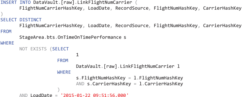
The loading process for links should only load newly arrived business key relationships from the source table in the staging area. For this reason, the insert statement is comparable to the hub statement, but is based on the hash keys from the referenced hubs and not on the business keys found in the source:
The SELECT part in this statement uses a DISTINCT clause again, in order to avoid checking the same business key relationship multiple times. All hash keys have been calculated in the staging area again, which is used to simplify the actual loading and increase the reusability of the hash computation. Only relationships that don’t exist in the target link table are inserted. Because link tables use more than one referenced hub, the statement uses a NOT EXISTS condition in favor to a NOT IN statement. The sub-query searches for relationships that consist of the same hash keys.
Similar to the use of the load date in the statement for loading hubs (refer to section 12.1.1), the previous statement is filtering the data to one specific load date. This is done in order to sequentially load the batches in the staging area to ensure that the deltas are correctly loaded into the data warehouse. Therefore, another statement is required to find out the available load dates in the staging area first, order them (the batch with the oldest load date should be loaded into the data warehouse first) and then execute the above statement per load date found in the staging area.
The statement doesn’t check the validity of the incoming links. For example, in some cases, the source system provides a NULL value instead of a business key. In this case, the above statement maps NULL business keys to a hash key, which is the result of the hash function on an empty string. In order to maintain the data integrity, this key has to be added to the hub, as well. However, there are two cases that might happen when loading business key relationships:
1.At least one expected business key was not provided: in this case, the source system provided erroneous data because an expected business key, which was used in a foreign key reference, was not provided and is NULL.
2.At least one optional business key was not provided: the business key in the source system is optional and was not provided. This is not an actual error.
It is important to cover both cases in order to analyze both errors and design issues. If only one extra hub record is used to cover the NULL business keys, it is not possible to distinguish between these cases. For that reason, there should be actually two extra records in the target hub (see Table 12.2).
Table 12.2
Ghost Records in Airport Hub Table
Airport Hash Key
Load Date
Record Source
Airline ID
1111…
0001-01-01 00:00:00.000
SYSTEM
-1
2222…
0001-01-01 00:00:00.000
SYSTEM
-2
1aab…
2013-07-13 03:12:11.000
BTS
JFK
The first record indicates the first option: the expected business key was not provided by the source. This is an actual error. The business key is set to an artificial, system-generated value, in this case −1. The hash key is set statically as well, because it makes the identification easier. It could also be derived from the artificial business key.
The second record is used for business keys that are optional and not provided. For this case, the business key −2 was artificially set. The hash key is set to 22222222222222222222222222222222 (32 times the character “2”). This way, it is easy to identify records in the source system that are attached to the missing key for some reason. The third record in the table is a valid business key.
When data is loaded from the source and cannot be associated with a business key, for example because the business key column in a source flat file is left empty, the data in the satellite is associated with one of these entries in the hub table. If a business key is missing in satellites on hubs, many of these cases are attached to the first option that covers missing business keys.
However, especially when loading link tables from foreign key references in the source system, both cases are very common. If a NULL reference is found in the source system, this information is added to the link table (Table 12.3).
Table 12.3
Linkconnection With Expected and Unexpected Null References
Connection Hash Key
Load Date
Record Source
Carrier Hash Key
Source Airport Hash Key
Destination Airport Hash Key
Flight Hash Key
87af…
2013-07-13 03:12:11
BTS
8fe9… {UA}
3de7… {DEN}
1111… {-1}
a87f… {UA942}
28db…
2013-07-13 03:12:11
BTS
8fe9… {UA}
3de7… {DEN}
1aab… {JFK}
8df7… {UA4711}
9de7…
2013-07-14 02:11:10
BTS
8fe9… {UA}
3de7… {DEN}
1aab… {JFK}
9eaf... {UA123}
9773…
2013-07-15 03:14:12
BTS.x
8fe9… {UA}
2222… {-2}
9bbe… {SFO}
821a… {UA883}
The first line describes a connection between Denver and an unknown destination airport. Because the record was expected but not provided by the source system, the hash reference into the airport hub is set to the hash key reserved for erroneous data.
The last record in Table 12.3 references the second reserved record in the airport hub, reserved for cases when an optional business key is not provided. This is not perfect, but also not an error.
In both cases, the incoming NULL value is replaced by the artificial business key from the hub, with the artificial hash key (or the hash key derived from the artificial business key). Once the link is loaded into the Raw Data Vault, it is possible to load satellite data that describes the erroneous or weird data. This descriptive data is typically found next to the foreign key reference, in the same source table.
By following this process, the data warehouse integrates as much data as possible and allows the data warehouse team and the business user to analyze any issues with the source system directly in the Raw Data Vault. The data will later be “cleansed” by business logic, when loaded into the information marts.
12.1.2.2. SSIS Example
Loading Data Vault 2.0 links in SSIS follows a similar approach to loading hubs. Because links can also be provided by multiple source tables (within the same source system), each source that provides link records desires its own data flow. After adding an OLE DB source transformation to the newly created data flow, open the OLE DB source editor (Figure 12.20).
Figure 12.20OLE DB source editor for loading links.
Select the StageArea database from the list of databases and set the data access mode to SQL command. Insert the following SQL statement into the editor for the SQL command text:
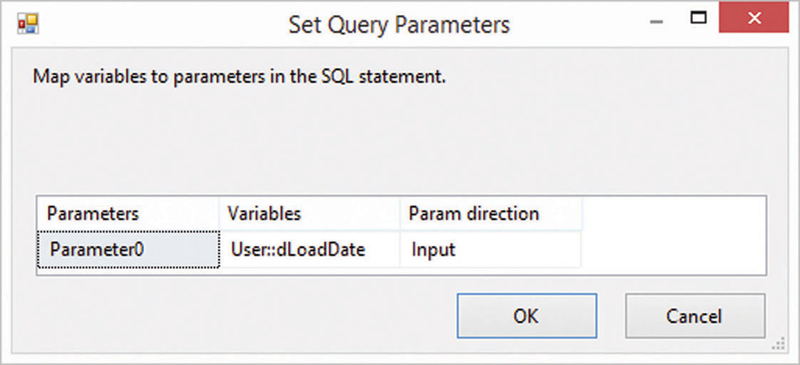
This statement selects all links for a given batch from the source table in the staging area. The batch is indicated by the load date. This approach follows the hub loading process and requires using the variable defined in section 12.1.1 (Figure 12.21).
Figure 12.21Set query parameter for load date timestamp.
Map the parameter in the SQL command text to a SSIS variable by selecting the variable in the second column. The param direction should be set to input as it is the default. Close the dialog. This completes the configuration of the source component. Drag a lookup component into the data flow and connect its input to the default output from the OLE DB source. Open the lookup transformation editor, which is shown in Figure 12.22.
Figure 12.22Set up the lookup transformation editor to find existing links.
Similar to the hub loading process, the process shown in this section is interested in links that don’t exist in the target table. That is why this lookup is performed against the target. To prevent a failure of the SSIS process, select redirect rows to no match output in the selection box. This will open another output that provides the unknown link structures that should be loaded into the target. Those that are already found in the target link table are ignored. This follows the link loading template outlined in section 12.1.2.
Switch to the connection page of this dialog by selecting the corresponding entry on the left side (Figure 12.23).
Figure 12.23Setting up the connection in the lookup transformation editor for link tables.
This page sets up the connection to the lookup table. Because the goal of the lookup is to find out which links don’t exist in the target table, select the DataVault database and the target table LinkFlightNumCarrier.
To complete the configuration of the lookup transformation, select the columns page on the left side of the dialog. The page shown in Figure 12.24 allows the configuration of the lookup columns and the columns that should be returned by the transformation.
Figure 12.24Configuring the columns of the link lookup.
Instead of using the hash key of the link (which is the primary key of the link table), the lookup should be performed on the hash keys of the referenced hubs. This improves the detection of hash key collisions. Because we’re only interested in finding out which links are not in the target table yet, no columns are returned from the lookup table.
Select OK to close the lookup transformation editor. Insert an OLE DB destination and connect the output from the lookup to the destination. Because there are multiple outputs due to the redirection of unknown links in Figure 12.22, a dialog (Figure 12.25) is shown to map the output to the input.
Figure 12.25Input output selection for link loading process.
The lookup no match output provides the link records from the source table in the staging area that have not been found in the target link table yet. Therefore, select this output and map it to the OLE DB destination input in order to load unknown link records to the target. The other output provides only link records that are already known to the target and will be ignored.
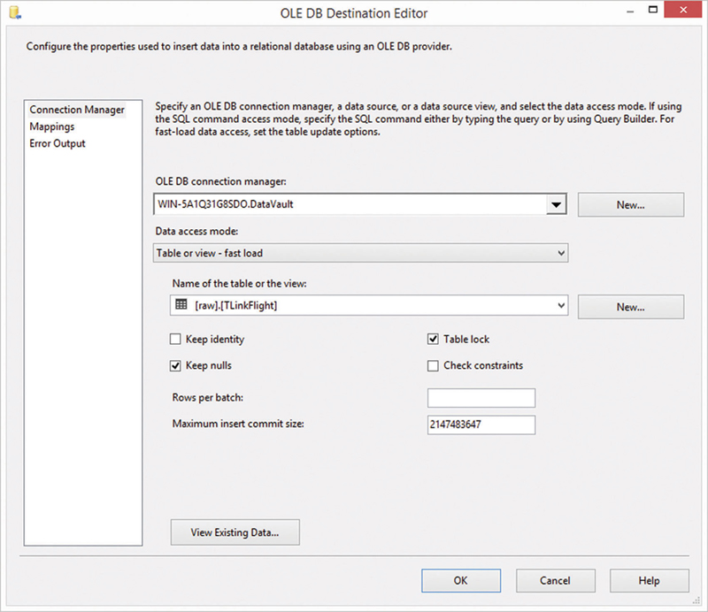
Close the dialog and open the OLE DB destination editor, shown in Figure 12.26.
Figure 12.26OLE DB destination editor for the link table destination.
Select the connection manager for the DataVault database and select the LinkFlightNumCarrier link table in the raw schema. Make sure that keep nulls and the table lock option are checked. Keep identity and check constraints should be unchecked for the same reasons as in the hub loading process. Consider changing the rows per batch and maximum insert commit size in order to adjust the SSIS load to your infrastructure.
Switch to the mappings page by selecting the entry in the list on the left of the dialog. The page shown in Figure 12.27 is presented.
Figure 12.27Mapping the columns in the OLE DB destination editor.
Make sure that each column from the destination is mapped to a corresponding column in the source. Close the dialog. The final data flow is presented in Figure 12.28.
Figure 12.28Data flow to load Data Vault 2.0 links.
This data flow might be extended by capturing errors in the error mart. Such an approach would follow the approach outlined in Chapter 10, Metadata Management.
12.1.3. No-History Links
The loading pattern for no-history links (also known as transactional links) is even simpler than the loading template for standard links (described in section 12.1.2). The only difference is that the lookup in the loading template becomes optional (Figure 12.29).
Figure 12.29Template for loading nonhistorized link tables.
Because no-history links are typically used for transactions or sensor data, one record needs to be loaded per transaction or event. It is not a distinct list of relationships. The lookup ensures that no duplicate transactions or events are loaded in the case of restarts.
This approach can be implemented in a fully recoverable approach, without the need to delete the partially loaded records in the target link table before restarting this process. While the process runs slower in the case of restarting the loading process (due to the lookup), it doesn’t need any special handling. The ETL process is just restarted and loads the remaining records into the target table.
12.1.3.1. T-SQL Example
From a structural perspective, the no-history link target to be loaded in this section is not different to any other link table in the Raw Data Vault. The only difference is the name, which starts with “TLink” instead of “Link”:
The no-history link consists of FlightHashKey as an identifying hash key (used in the primary key), a load date and record source and the hash keys of the referenced hubs: HubFlightNum, HubTailNum, HubAirport. The latter was referenced twice and two hash keys are stored: one for the origin airport and the other for the destination airport.
The source data provides no unique event or transaction number: the flight data itself is not a good candidate to be used as a transaction or event number in the non-historized link. But such a number is required to achieve the proper grain, which fits the grain of the actual flights. Using only the hub references is not enough, because the flight number is reused from one day to the other. The goal is to achieve two goals for the loading process of no-history links:
1.Same grain as transactions or events: each transaction or event should have one record in the no-history link table in order to easily source fact tables from this table.
2.Unique hash key for primary key: the hash key in a link table is based on the referenced business keys. In order to achieve the first goal, another identifying element is required because, in most cases, the hub references alone have another grain than the transactions themselves (think of reoccurring customers, buying the same product in the same store).
Because no such transaction number is available in the source data, the flight date is added. It is not unique by itself, but fits the purpose of achieving the required grain and producing a unique hash key for the link when the date is included in the hash key calculation. The underlying elements, that is the hash keys of the referenced hubs and the flight date, are included in the alternate key for uniqueness and to speed up (optional) lookups.
Because the flight date was already included when calculating the hash key in the staging area, it is possible to simply load the data from the staging area into the no-history link:
Also, the order in which the data is loaded into the link table doesn’t matter, that’s why there is no filter for a specific load date. All the data is simply loaded into the target table. To achieve a recoverable process, a lookup is required that checks whether the record to be loaded is already in the target table. The NOT EXISTS condition in the WHERE clause is taken from the statement to load standard link tables. Note that the flight date was included in this condition to make sure that duplicates are filtered out accordingly.
12.1.3.2. SSIS Example
To implement the T-SQL based loading process from the previous section in SSIS, a similar data flow is required to the previous SSIS example for loading Data Vault 2.0 links. Drop an OLE DB source transformation to a new data flow and open the editor (Figure 12.30).
Figure 12.30OLE DB source editor for no-history links.
The OLE DB source transformation loads the data from the source table in the staging area by using the following SQL command text:
Because the flight date in the source table is stored as an nvarchar, it is converted into the correct data type on the way out of the staging area and into the Raw Data Vault no-history link table. This is the latest point that it should be done. If possible, it should already be done in the staging area, but in some cases (refer to Chapter 11, Data Extraction), it has to be done on the way out. The load date is also included in this statement to process only one batch at a time. As usual, use the Parameters… button to map the parameter to a SSIS variable (Figure 12.31).
Figure 12.31Set query parameter for nonhistorized link.
Once the load date variable has been mapped to the parameter, close the dialog and the OLE DB source editor. Insert a lookup transformation into the data flow and connect it to the output of the OLE DB source. Open the lookup transformation editor, shown in Figure 12.32.
Figure 12.32Lookup transformation editor for no-history links.
Again, make sure that redirect rows to no match output has been selected in the combo box on the first page. After that, switch to the next page by selecting connection from the list on the left of the dialog. The page is used to set up the target transaction link as the lookup table (Figure 12.33).
Figure 12.33Setting up the connection in the lookup transformation editor for no-history links.
Make sure that TLinkFlight in the raw schema of the DataVault database is used for the connection and switch to the columns page of the dialog (Figure 12.34).
Figure 12.34Configuring lookup columns for the no-history link.
Similar to the standard link, the hash keys of the referenced hubs are used to perform the lookup. However, because the hash keys alone are not enough to correctly identify the link, the flight date is added into the equi-join of the lookup as well. No columns from the lookup table are returned because we’re only interested in finding out if the no-history link already exists in the target or not.
Close the dialog and add an OLE DB destination to the data flow. Connect the output path from the lookup transformation to the destination transformation. Because unknown links are redirected into another output, the dialog shown in Figure 12.35 appears.
Figure 12.35Input output selection for no-history links.
Select the lookup no match output because it contains all the records where no corresponding link record has been found in the target link table.
Close the dialog and open the OLE DB destination editor, as shown in Figure 12.36.
Figure 12.36OLE DB destination editor of the no-history link.
Select the target table, TLinkFlight in the raw schema of the DataVault database, and make sure that keep nulls and table lock are checked. The other options (keep identity and check constraints) should not be checked. Rows per batch and the maximum insert commit size should be adjusted to your data warehouse infrastructure. Check that the column mapping of the data flow to the destination table is correct by switching to the mappings page of the dialog (Figure 12.37).
Figure 12.37Mapping columns in the OLE DB destination editor of the no-history link.
Each destination column should have a corresponding input column. Select OK to confirm the changes to the dialog.
Figure 12.38 presents the final SSIS data flow for loading no-history links.
Figure 12.38Complete SSIS data flow for loading no-history links.
In addition to this link table, no-history links often have nonhistorized descriptive data stored in no-history satellites. Their loading process is covered in one of the coming sections on loading satellite entities.
12.1.4. Satellites
While the loading templates for hubs and links, even for special cases such as no-history links, are fairly simple, satellites are a little more complicated. However, the loading template for satellites follows the same design principles as discussed in the introduction to this chapter, thus becoming a fairly simple template as well.
The goal of the satellite loading process is to source the data from the staging area, find changes in the data and load these changes (and only these changes) into the target satellite. The default loading template for satellites is presented in Figure 12.39.
Figure 12.39Template for loading satellite tables.
The first step is to retrieve a distinct list of records from the staging table that might be changes. This step should omit true duplicates in the source because the satellite wouldn’t capture them anyway. By doing so, the data flow reduces the amount of data early in the process, following the design principles for the loading templates.
Note that we define true duplicates as actual duplicates that are added to the staged data due to technical issues and provide no value to the business. We assume that these records should not be loaded into the Raw Data Vault and are filtered out in the loading process. If duplicates should be loaded, consider using a multi-active satellite for this purpose (refer to Chapter 5, Intermediate Data Vault Modeling, for more details).
Once the data (which contains both the descriptive data as well as the hash key of the parent hub or link table) has been sourced from the staging area, the latest record from the target satellite table that matches the hash key is retrieved. This step is easy, because the latest record should have the latest load date of all the records for this hash key and a NULL or maximum load end date.
Both records, the record from the staging area and the latest satellite record obtained in the previous step, are compared column-wise. If all columns match, that means that no change has been detected, and the record is dropped from the feed because the satellite should not capture it. Remember that Data Vault satellites capture only deltas (new or changed records). If a record has not changed, it is not loaded into the satellite table.
If there is a change in at least one of the columns, the record is added to the target satellite table. Note that, in most cases, the change detection relies on all columns. However, there might be cases where some of the columns are ignored during column comparison. This would result in undetected changes. If all other columns were unmodified, no record would be added. Therefore, such a limited column comparison should be used only in specific and rare cases. Another thing to consider is if the column comparison should be case sensitive or case insensitive. Depending on the source data, both options make sense and are frequently used.
The major issue with the column comparison is that satellites sometimes contain a large number of columns that are required to be compared. This comparison can take time, especially if the number of records in the stage area that might contain changes to be captured is high as well. In order to speed up the performance of the loading template presented in Figure 12.39, hash diffs can be used. The hash diffs have been introduced as optional attributes to satellites in Chapter 4 and explained in great detail in the previous chapter.
Once the hash diff has been added to the satellite entity, it can be used to compare the input record with the target record with a comparison on one column only. When loading the Data Vault satellite, both required hash diffs from the source and the target are already calculated. The source data has already been hashed in the staging area, while the target satellites have the hash diffs included for each row by design.
Because of this preparatory work, the modified loading process doesn’t require any hashing and is merely a simplified version of the standard loading template for satellites (Figure 12.40).
Figure 12.40Template for loading satellite tables using hash diffs.
The difference between both loading patterns is only in the comparison step that either drops the record from the feed or loads it into the target table. This comparison is reduced to compare the hash diffs instead of all individual columns. It also removes the need to account for NULL values as this has been done in the hash diff calculation already by replacing the NULL values with empty strings in conjunction with delimiters. Other than the changed comparison, the template is the same as in Figure 12.39.
12.1.4.1. T-SQL Example
This section loads the descriptive data for the airports. However, there are two different sets of columns, each describing either the airport of origin or airport of destination. This data could be merged into one satellite, but aligning it might require additional business logic: what happens if data from both sets of columns contradict each other, e.g., using different descriptive data for the same airport and the same load date time? The load processes of the Raw Data Vault should not depend on any conditional business logic. Therefore, both sets of descriptive data are distributed to different satellites, each hanging off HubAirport. The first satellite captures the descriptive data for the originating airport and is created using the following DDL statement:
The satellite contains the parent hash key and the load date in its primary key. The load end date is NULLable and indicates if and when the record has been replaced by a newer version. The descriptive “payload” of the satellite is defined by the columns OriginCityName, OriginState, OriginStateName, OriginCityMarketID, OriginStateFips and OriginWac. Because the primary key contains a randomly distributed hash key, a nonclustered index should be used.
Note that this satellite does not use the hash diff value calculated in the staging area for demonstrative purposes. The next satellite, also presented in this section, uses the hash diff value.
It is easily possible to implement the template shown in Figure 12.39 in T-SQL only:
This statement selects the data, including the parent hash key, the load date, the record source and the descriptive data from the source table in the staging area. The select is a DISTINCT operation because the airport is used in multiple flights (most airports serve multiple flights per day). If the DISTINCT option is left out, duplicate entries would be sourced and the subsequent insert operation would violate the primary key constraint of the target satellite. The load end date is explicitly set to NULL for demonstration purposes. As an alternative, it could also be removed from the list of columns and set implicitly. Because only changed data should be sourced into the target satellite, each column from the source stage table needs to be compared with its corresponding column in the target satellite table including a check for NULL values in the descriptive columns. This check could also be implemented using the ANSI-SQL standard function COALESCE. This column comparison is implemented in the WHERE clause of the statement. It requires that the target satellite be joined into the statement in order to have the current target values available. For this reason, a LEFT OUTER JOIN is used to join the data into the source dataset. The join condition compares both hash keys of the parent and requires that the record should be active. The latter is checked by selecting only records from the target with a load end date of NULL. When comparing the records, only new and active records with a load end date of NULL are interesting.
The additional filter on the source load date ensures that only one batch is loaded. This is very important in the loading process of satellites because the delta detection depends on the fact that only one batch is evaluated at the same time. Changing this is possible but complicates the process. Also, it is important to run the batches in the staging area in the right order, to make sure that the final satellite has captured the changes as desired.
The second satellite, SatDestAirport, which captures the descriptive data for the flight’s destination airport, uses the hash diff value to improve the performance of the column comparison. Therefore, the hash diff column was added to a structure similar to the SatOriginAirport:
The technical metadata of the satellite, including the parent hash key AirportHashKey, the load and end date and the record source, are exactly the same as in the previous satellite table. In addition, the hash diff column was added and the names of the descriptive columns are slightly different, due to different names in the source table.
To load the data from the source table in the staging area into the target satellite table, the following statement is used:
The only difference from the previous INSERT statement, apart from the fact that it loads the table SatDestAirport instead of SatOriginAirport (thus sourcing different columns from the staging table), is that the column compare was simplified: only one column is compared instead of all descriptive columns. If the hash diff in the target is different from the one in the stage area, or if there is no record in the target satellite that fits to the hash key (which leads to a hash diff of NULL), the record is loaded into the target.
Both INSERT statements rely on an OUTER JOIN in order to join the data into one result set. This is required in order to compare the incoming data with the existing data or produce NULL values if there is no satellite entry with the same parent hash key as the incoming record. If another join type is used, the column compare would not compare a wrong record or data would be lost on the way from the staging table to the Raw Data Vault. If the performance of the loading process is too slow due to the OUTER JOIN, the best approach is to divide both datasets (the new and the changed records from the staging area) and process them separately. This is covered in section 12.1.6.
The descriptive data in both satellites can be combined later in the Business Vault, for example using PIT tables or computed satellites. These approaches are covered in Chapter 14, Loading the Dimensional Information Mart.
12.1.4.2. SSIS Example
It is also possible to implement the loading template for satellites using SSIS. This approach also requires the load date variable in the SSIS package to ensure that only one batch is loaded into the Raw Data Vault during a single SSIS execution.
The first step is to set up the source components in the SSIS data flow. Unlike the SSIS processes for hubs and links, the SSIS data flow presented in this example uses two different source components from different layers of the data warehouse:
1.The source staging table: this table provides the new and changed records along with unchanged records.
2.The target satellite table: this table provides the current version of the data in the target.
The data from both sources will be merged in the data flow and compared during column comparison. Essentially, this approach implements a JOIN operation instead of a lookup (sub-query in T-SQL) for performance reasons. The first source component, an OLE DB Source, is set up using a SQL command, as Figure 12.41 shows.
Figure 12.41Set up the source component for the staging area data source.
The following SQL statement is used as SQL command text:
There are two lines noteworthy: first, the ORDER BY clause is required for the merge operation of both data sources because it improves performance if the key that is used for merging the data streams already sorts both data flows. In this case, this will be the hash key. The second interesting line is the use of the WHERE clause to load only one batch from the staging area, based on the variable defined earlier. The parameter is referenced using a quotation mark in the SQL statement. In order to associate it with the variable, use the Parameters… button. The dialog shown in Figure 12.42 is presented.
Figure 12.42Set query parameters dialog.
Select the variable previously created and associate it with the first parameter. Select the OK button to complete the operation. Close the OLE DB Source Editor to save the SQL statement in the source component. However, the component is not completely set up yet. While the incoming data is ordered by the hash key to optimize merging the data flows, this setting has to be indicated to the output columns of the source component in addition.
Open the advanced editor from the context menu of the source component (Figure 12.43).
Figure 12.43Advanced editor of source component.
Select the OLE DB Source Output node in the tree view from the left. Set the IsSorted property of the output to true. The last setting is to indicate the actual column that was used for sorting. Select the column from the Output Columns folder in the tree view, as shown in Figure 12.44.
Figure 12.44Setting the SortKeyPosition in the advanced editor.
Set the SortKeyPosition property to the column number of the hash key in the source query. Because the hash key is the first column in the SQL statement used in Figure 12.41, the position value 1 is set.
This completes the setup of the staging table source. The next dialog shows the setup of the source component that sources the data from the target satellite, which is required to compare the incoming values with the existing values (Figure 12.45).
Figure 12.45Source Editor for target data.
The following SQL statement is used as the SQL command text:
The statement loads all records from the target satellite, which are currently active (having a load date of NULL). The data is also ordered to enable merging the data flows in the next step. Because the data is ordered, this has to be indicated to the SSIS engine using the same approach by setting the IsSorted property of the output and the SortKeyPosition of the hash key output column as described in Figure 12.43 and Figure 12.44.
Once the data from both sources is available in the data flow, the next step is to merge both data streams in order to be able to compare the values from both the staging area and the target satellite. Drag a Merge Join Transformation to the data flow canvas and open the editor (Figure 12.46).
Figure 12.46Merge join transformation editor.
There are two tasks to complete in this dialog: first, the columns that are used for the merge operation have to be connected. In this case, this is the hash key from each data stream because the streams are merged on this value. Drag the OriginHashkey column over the AirportHashKey in order to connect both columns. Also, make sure that the join type is set to left outer join. The second task is to select the columns that should be included in the merged data stream. This should include all columns from the staging area and the descriptive data from the target satellite because all of this data is required for either the column compare or the loading of the target satellite table. Because the descriptive columns are named the same in both the source and the target, rename one or both sides as in Figure 12.46.
Close the dialog and drag a conditional split transformation to the canvas of the data flow. This component is used to filter the records from the staging area source that don’t represent a change from the data that is already in the target satellite (Figure 12.47).
There should be two outputs configured in this dialog: one output for records that are new or changed and should be loaded into the target satellite and another output for the records that do not represent a change and should be ignored. The first is configured by adding another output to the list of outputs in the center of the dialog and setting the following condition:
This condition implements a columnar-based, case-sensitive compare operation that takes potential NULL values into account. In order to implement a case-insensitive version of this operation, the expression should be extended by UPPER functions on all columns from both the staging area and the target satellite. It is also important to take special care for columns with a float data type. If any of the fields in the payload are flow, then converting them to a string zero without a forced numeric (fixed decimal point) may actually fail the comparison for equality.
The default output is left as is and is responsible for dealing with the records that are already known to the target satellite. These records will be ignored.
Close the dialog and drag an OLE DB destination to the canvas. Connect the conditional split transformation to the destination component by dragging the data flow output of the conditional split transformation to the destination. The dialog in Figure 12.48 will be shown to let you select the desired output that should be written into the destination.
Figure 12.48Input output selection dialog.
Select the changed records output from the conditional split transformation and the OLE DB destination input from the OLE DB destination component. Select the OK button to close the dialog. Open the OLE DB destination editor to set up the target (Figure 12.49).
Figure 12.49OLE DB destination editor.
On the first tab, select the target satellite table. Because NULL values should be written into the target, it is important to check the keep null option. To ensure highest performance, table lock should be turned on. Parallel loading of the same satellite table should not be required because the recommendation is to load only data from one source system into a satellite (separate data by source system). The other options should be adjusted; especially the rows per batch and the maximum insert commit size option. Check constraints should not be necessary as they often implement soft business rules, which should be implemented later.
Select mappings from the left to edit the column mappings from the columns in the data stream to the destination table columns (Figure 12.50).
Figure 12.50Mapping the columns from the data stream to the destination.
Because the columns in the data flow and in the destination table use the same name, the mapping editor should have mapped most columns already. Make sure that each destination column except the load end date has a source column. The load end date is left NULL for now because end-dating is separated from this process and is covered in section 12.1.5. In most cases, the hash key needs to be mapped, because the name often differs in the source and the target table.
This completes the setup of the loading process for satellites. The complete data flow is presented in Figure 12.51.
Figure 12.51Satellite loading process based on column compare.
The final loading process presented in the figure can be optimized by comparing the source data with the target data based on the hash diff value instead of each individual column value. In order to do so, the hash diff values have to be included in the data flow and used in the conditional split transformation instead of the individual column values. Therefore, a couple of modifications are required to the data flow presented before. In the following example, the previous data flow has been copied and adopted for another target satellite SatDestAirport.
Open the OLE DB source editor for the source table in the staging area (Figure 12.52).
Figure 12.52OLE DB source editor for destination airport staging data.
In this dialog, copy and paste the following SQL statement into the SQL command text editor:
Make sure that the parameter is still bound to the load date variable previously created. Notice that the metadata of the output is out of sync when closing the dialog. Double-click the path in the data flow and select delete unmapped input columns to fix the issue.
Open the editor for the second source on the target satellite table (Figure 12.53).
Figure 12.53OLE DB source editor of the target satellite table.
Because the payload of the target satellite is not required for the delta checking, remove all descriptive columns from the SQL command text and add the hash diff column:
No other columns except the parent hash key and the hash diff values are required from the target. However, make sure that only active records are returned by limiting the result to records with a load end date of NULL.
After closing the dialog, fixing the metadata of the path in the data flow might be required for this source as well. Also make sure that both sources have IsSorted set to true for their output and the SortKeyPosition of the respective hash key column is set to 1.
The next task is to fix the merge join by using the merge join transformation editor, shown in Figure 12.54.
Figure 12.54Merge join transformation editor for hash diff column compare.
Make sure that the hash key from the staging area is mapped to the hash key in the target satellite table. In Figure 12.54, the DestHashKey is mapped to the AirportHashKey. In addition, select all columns from the staging area, because they contain the descriptive data that should be loaded into the target satellite. In order to check if any columns have changed, add the hash diff column from the target satellite to the data flow.
Close the dialog and open the editor of the conditional split transformation (Figure 12.55).
Figure 12.55Conditional split transformation editor for delta checking based on hash diff.
Replace the condition in the dialog shown in Figure 12.55 by the following expression:
This expression only uses the hash diffs from the source and the target to perform the delta checking. It takes possible NULL values in the target hash diff into consideration to ensure that new records are loaded as well (they don’t have a corresponding record in the target, thus their target hash diff is NULL).
Finally, the OLE DB destination has to be set up. Figure 12.56 shows the first page that sets up the table.
Figure 12.56OLE DB destination editor for SatDestAirport.
Change the name of the target to SatDestAirport. Make sure that keep nulls are enabled and switch to the mappings pane (Figure 12.57).
Figure 12.57OLE DB destination editor for mapping the source columns to the target.
Make sure that all descriptive columns are mapped to the target and that the hash diff value from the source table in the staging area is mapped to the hash diff column of the target satellite. This is important to ensure that the hash diff is available when running this process another time.
Figure 12.58Complete data flow for loading satellites using hash diffs.
In addition to the presented setup, a production-ready loading process would write erroneous data from the source into the error mart if it fails to load the data. In order to add the error mart to the data flows presented in this section, send error outputs to OLE DB destinations for the error mart as described in Chapter 10, Metadata Management.
12.1.5. End-Dating Satellites
The standard loading process of satellites is not complete yet. After the loading process for a satellite has been completed, there are multiple satellite entries active: two or more records have a load end date of NULL or 9999-12-31. This is invalid because there should be only one record active in a consistent Data Vault satellite (except for multi-active satellites). Therefore, an end-dating process is required after having loaded the data of one batch (one load date) from the staging table into the target satellite. The overall process is presented in Figure 12.59.
Figure 12.59Template for setting the load end-date in satellite rows.
The first step in this process is to retrieve the data from the satellite table. Once the records have been retrieved, the records are sorted per group and per load date (descending) in the second step.
Within each group, the first record needs to be calculated (step 3) because this record should remain active. Therefore, the process sets the load end date to NULL for this record (or makes sure that this record keeps its NULL or future load end date). After that, the load end-dates of the remaining records are calculated for each group. This process is described next. Once all load end-dates are calculated, the target satellite is updated with the new load end-dates and the process completes.
Note that the sort operation in the second step of this process forces the use of the tempdb database in Microsoft SQL Server if the process is implemented in SQL Server. If implemented in SSIS, the sort operation will release the lock on the source component’s connection of the satellite table.
The subprocess to calculate the load end-dates is shown in Figure 12.60.
Figure 12.60Calculate load end-date for remaining records subprocess.
In the first step, the incoming record set is reduced to those groups of data per parent hash key which have more than one active record per group. Active records are defined by records with a load end date of NULL or 9999-12-31 (the future date). All other records are not of interest for this process, because if there are not at least two active records per parent hash key, the single record has to remain open and, therefore, remains untouched.
After these records have been removed, each group is ordered by load date. This is achieved by ordering the whole data flow by hash key (to group all records belonging to one parent hash key together) and load date (descending). Ordering the load dates in a descending order is important because the process has to calculate “carry over” values for each record. This process is shown in Figure 12.61.
Figure 12.61Calculate load end-date walkthrough.
The first table on the left includes four parent hash keys. Only the data that belongs to the hash keys 2abcff… and 4444dd… are processed by this template because the other two hash keys don’t have more than two active records in the satellite. For example, the data for the parent hash key 1bef79… consists of one active record and one record already end-dated in the past. Once the data has been filtered out, the data is sorted by hash key and load end-date in the second step. The result is shown in the upper-right table.
Then, the “carry-over” value is calculated for each record within the group, except the first one (which should remain active). Each record except the first in the group should have a load end-date set to the load date of the next record in the group (ordered on a time-scale). Because of that, the load date of the newer record is copied over to the next older record, as shown in the lower-right table of Figure 12.61. Once all load end-dates have been set, the data is sent as updates to the target satellite.
The following T-SQL statement can be used to perform the end-dating process:
This statement end-dates the satellite SatPreferredDish. It assumes open satellite entries (records which are not end-dated yet) to be are indicated by a NULL LoadEndDate. The sub-query in the statement retrieves the LoadDate of the next entry for each PassengerHashKey. By doing so, it implements the process as outlined in Figure 12.61.
The previous statement should be executed for each parent hash key individually, in order to ensure that it scales to higher amounts of data. While the statement is not a fast approach, the statement scales linearly on the number of parent hash keys. If the load end-dates of all hash keys are updated at once, in a single transaction, the resource requirements could become too high and the database server may start to swap data out of memory to disk in order to deal with the amounts of data. Depending on the database management system used, other approaches than the one presented in the previous statement are more feasible as well.
The process of end-dating the satellite data has been separated from the loading process in order to deal with each problem separately. This simplifies the loading process and ensures that the performance remains high. Another important issue is that the statement deals with all the whole group of data per parent hash key at once, in order to make sure that previously loaded data becomes end-dated as well. This is important because a previous loading process might have been aborted and may left the satellite data in an inconsistent state. Therefore, this separation becomes part of the restartability characteristics of the Data Vault 2.0 loading patterns.
12.1.6. Separate New from Changed Rows
The performance of the templates shown in the previous section relied on the separation of duties to some extent. For example, several operations have already been conducted in the staging area, such as hashing. Other operations are performed once the data have been loaded, such as setting the load end-date but also performing any recalculations.
The performance of the above templates can be improved further by more separation. This relies on the fact that the column comparisons are only required for parent hash keys that are already known to the satellite, i.e., potential updates to the same hash key. If the source system contains a record that describes a business key or business key relationship that is already known to the data warehouse, the column comparison is used to find out if the source system has changed between the loads.
But if the source system described a business key that is unknown to the satellite, the column comparison is not required: there will be no record available in the target that could be used in the update detection process. The new record has to be loaded into the target satellite in any case.
The previous templates always perform the column comparison. If SQL is used to implement the template, the compare might require an outer join because changed rows are detected using direct index match. But even if ETL is used, the column comparison is not required and reduces performance of the overall load. Therefore, it is possible to improve the performance of the satellite loads by separating new and changed records. This is especially useful if the number of new records in the source system outweighs the number of changed records. The programming logic that is required to detect changes should not be applied to new records because it reduces the performance of the loading pattern.
The first resulting template, which loads changed rows from the staging table only, remains mostly unchanged to the default satellite loading template in section 12.1.4 (Figure 12.62).
Figure 12.62Template for loading only changed records into satellite tables.
The only difference is in the first step because it only loads changed records from the staging tables. But implementing this step requires the identification of records that have potentially changed directly in the staging area. However, this is easy to do if the staging area is on the same infrastructure as the rest of the data warehouse. In this case, it is possible to do the source query on the staging area and perform a look-ahead into the target to identify which hash keys are already known to the data warehouse:
This statement shows that the staging area is not only used to reduce the workload on the source systems, but it can also be used to perform intermediate tasks that improve the performance of the data warehouse loading processes. And it shows the additional value of having calculated the hash keys in the staging area: it does not only improve the reusability of the hash computations, but can also be used to improve the loading processes even further (as described in this section).
In order to load the new records only, the loading template in Figure 12.62 can be greatly simplified because no change detection is required by the loading process anymore (Figure 12.63).
Figure 12.63Template for loading only new records into satellite tables.
Not only is the column compare removed, but also the retrieval of the latest record from the target satellite table. New records are just loaded into the target. This template also requires that the source query on the staging area provides only new records with hash keys unknown to the target satellite:
Both processes for new and changed records can run in parallel, because they operate on different sets of input data which are loaded into nonoverlapping primary keys of the target table (again, because the processed hash keys of each ETL process are different).
12.1.7. No-History Satellites
The approach described in the previous section can also be used to load nonhistorized satellites. The reason is that the no-history satellite does not track changes in the source system. Instead, there are only new records that need to be loaded into the target table. Because of that, the same template as presented in Figure 12.63 can be used for loading satellites with no history.
The following DDL statement creates a no-history satellite in the Raw Data Vault:
There is no load end date in the satellite structure because changes are not tracked. For the same reason, the load date has been degraded to technical field without any importance for the model. The primary application is to be used during debugging: it exists in order to understand when data was loaded into the target. However, there is a secondary application to it: when incrementally loading subsequent information marts, it is helpful to load only new records into the information mart layer. This is why the load date was included in the primary key constraint: by doing so, the field is used for indexing, which improves the load performance of the information mart.
Before the data can be loaded to the information mart, which is described in Chapter 14, the data has to be loaded from the staging area into the no-history satellite. The following statement can be used for this purpose:
This statement implements a simple copy process. Restartability is guaranteed by adding a LEFT OUTER JOIN that checks if the hash key of the parent no-history link is already in the target satellite. If this is the case, the record from the staging area is ignored, otherwise loaded. The load date is not required for this join, because there should only be one record per parent hash key in the target satellite.
12.1.8. Soft-Deleting Data in Hubs and Links
The processes presented in sections 12.1.1 and 12.1.2 load business keys or relationships between business keys into the data warehouse that have been inserted into the operational source system since the last batch. However, business keys are not only inserted into the data warehouse; they are also changed or deleted. Changing business keys is more of a business problem and requires special care up to the extent of asking the question whether the business key that is loaded into the hub is actually the right business key. Review the requirements for business keys in Chapter 4.
However, deleting keys is a common and valid operation and happens frequently. A product is removed from the catalog and not offered anymore, users lose access and their user account is removed from the operational system, etc. The same applies for relationships: employees quit and hire on with a new organization, products are moved into another category, and so on. In all these cases, the business demands that these changes be loaded into the data warehouse to be available for analysis. But the data warehouse doesn’t only reflect the current state of the data, but also the complete, nonvolatile history of the business keys, their relationships and all the descriptive data. For this reason, historic data usually cannot be deleted from the data warehouse.
Hubs and links play a vital role in the Data Vault 2.0 model to integrate the data of the data warehouse. If business keys are deleted from hubs or business key relationships are deleted from links, this integration breaks because descriptive data is stored in dependent satellites and references these business keys or relationships. Therefore, deleting records from hubs or links is not an option if the model is to remain intact.
The same applies to end-dating hubs and links. This approach would require a load end date in hub and link tables and could be used to end the employment of an employee with a specific company, for example. However, this approach introduces another problem (among others): what if the employee realizes that the new company was a bad choice and returns to the old organization? The HR people in the organization don’t care that hiring back the employee would break the Data Vault model due to duplicate keys in link tables.
The solution is to use effectivity satellites, introduced in Chapter 5, Intermediate Data Vault Modeling, to model such effectivity dates. The hub only provides information as to which business keys ever existed in the source systems and the link table provides the information about all relationships that ever existed. The corresponding effectivity satellite on the table provides the information about the effectivity that is the start and the end date of the business key existence or relationship validity.
Actually deleting data from the data warehouse is only performed when legal or privacy requirements have to be met, for example in a data destruction strategy.
12.1.8.1. T-SQL Example
The following DDL creates an effectivity satellite which is used to track the validity of an airline ID:
Because the satellite is dependent on the HubAirLineID, it includes the hash key from its parent hub and the load date of the record in the primary key. In addition, the table definition includes a load end date and the record source as technical fields. By doing so, it follows the definition of a standard Data Vault 2.0 satellite and treats the dates in the payload (ValidFrom and ValidTo) as ordinary descriptive fields, which can be changed by the source system at any time. This is called bi-temporal modeling [1].
The other two fields in the payload of the satellite, year start and year end, are the actual raw data fields from the source table. They have been used to calculate the ValidFrom and ValidTo fields in the loading statement of the effectivity satellite:
This statement aligns the data type of the integer-based year data in the source system to the required timestamp by applying the DATEFROMPARTS function on both year start and year end columns. Because this is a data type alignment only without recalculating the value, it counts as a hard rule and can be applied when loading the Raw Data Vault. However, in order to be able to trace errors, the original values are stored along with the aligned values, as well. Other recalculations should be avoided to include in the loading procedures of the Raw Data Vault and moved into the Business Vault or the loading processes of the Information Marts. If the source data changes, the satellite captures this change just as it does any other descriptive data.
Note that the above example relies on a table that has been artificially created and is based on the carrier history entity in the example MDS entity on the companion Web site. The MDS table contains multiple entries per carrier, which was simplified for demonstration purposes. The resulting table was placed in a custom schema.
12.1.9. Dealing with Missing Data
The problem with deleted business keys and relationships is that it is not always possible to detect actual deletes properly: under some circumstances, the source feed might not provide a business key that is actually in the source system. There are various reasons why a business key or other data is missing from the source:
•Source system not in scope: the source system simply isn’t being loaded to the data warehouse, for example when the source system did not deliver its exported source files to the data warehouse (due to a different schedule, for example).
•Technical error: in other cases the data exists in the source system, but is not exported, for technical reasons. The export could fail because there is no disk space left on the target disk for the export.
•Source filter: a source filter could have prevented the export of the data into the source file, even though the data is in the source system. When using delta loads, for example, only new data is exported into the file. Data that hasn’t changed at all is not being exported in such settings.
•ETL loading error: sometimes, data is not loaded into the staging area, even if the data is in the source files. This could be due to implementation errors in the ETL loading routines.
For these reasons, it is not guaranteed that a business key has been deleted from the source system just because it is not loaded into the stage area. However, we’d like to know which records have been actually deleted in order to mark them as such (so called “soft deletes”) in the data warehouse. Typically, this happens in effectivity satellites on hubs and links, as described in the previous section. In order to do so, we need to distinguish between data that has been left out of the source file for accidental reasons or by user action: that is, the record has been actually deleted from the source system.
In the best case, the source system provides an audit trail that tells the data warehouse what has happened to the source data between loads. This is the case when change data capture (CDC) has been activated in the source system and the CDC data is provided to the data warehouse as an audit trail. In such a case, the approach as outlined in section 12.1.8 can be used to load effectivity satellites from these sources.
However, in many cases, such an audit trail is not provided by the source system. Instead, a deleted record just disappears from the source data. It is not possible to distinguish between data that has been not provided by the source system and truly deleted data.
In order to solve this issue, the naïve approach is to retrieve all keys from the hub table and check if the hub keys are provided by the staging area (Figure 12.64).
Figure 12.64Full table scan required to detect deletes in the source system.
This assumes that the staging area provides a full load and not a delta load of the incoming data. If this is the case, the business key still exists in the source system and it is clear that it hasn’t been deleted. On the other hand, if the staging area doesn’t provide the key, it could be assumed that the key doesn’t exist in the source system anymore and therefore marked as deleted in the accompanying effectivity satellite.
The problem with this approach is that it requires many lookups, especially if the hub table contains a lot of business keys. For each key, the lookup into the source table has to be executed. In order to detect a deleted business key in hubs or deleted relationship in links, the process has to find the data that meets the following criteria:
1. The business key from the hub (or the relationship from the link) is not available in the source
2. The business key is not already soft-deleted in the target hub or link.
However, because of the full-scan on the target table, this process becomes unsustainable when the data grows. Instead of checking to see whether each hub key is still in the source table, the process should avoid the full-scan on the target table.
There is no solution to distinguish the missing and deleted business keys with 100% security. The best approach is to make an educated guess. The last seen date helps to make such a guess. This column is added to hubs (and links) where needed and used to build an inverted index tree. It is used only when CDC or an audit trail is not available from the source system (Figure 12.65).
Figure 12.65Introducing the last seen date in the loading process.
The last seen date is used to track when the business key stopped appearing on the feed to the data warehouse. By using this system-driven attribute, it is possible to minimize the data set that is required to scan. This approach works only on hubs and links. It is not intended to be used with satellite tables.
12.1.9.1. Data Aging
The last seen date helps to manage or reduce the table scan to a maintainable and viable set by introducing data aging (Figure 12.66).
Figure 12.66Data aging.
There are four data sources in Figure 12.66: flights, passengers, carriers, and airports. No source provides an audit trail and might have missing data. To simplify the problem, each source provides only one business key in this example. In the first week, the flight system, the carriers and the airports system provide “their” business key to the data warehouse. In the second week, flights and airports keep providing the key, but the carrier key is gone. Instead, the passenger key is provided. In the third week, only the carrier key is provided, and all others are missing. In week four, only the airport key is delivered to the data warehouse.
The data warehouse needs to find out which of the keys have been deleted and disappeared from further loads and which business keys are only missing from some loads. The carrier and airport keys are such examples, but also the passenger key that will appear in week five again. The flight key, on the other hand, seems to be deleted, because it doesn’t appear anymore. However, what if it appears in week eight?
The answer to this question cannot be given from the data warehouse team. Instead, the business has to answer this question. For each key, there might be different requirements. For example, the carrier key might be considered as deleted if it doesn’t appear for three weeks. This is due to the fact that the source system is relatively unreliable delivering the data to the data warehouse. On the other hand, the flights system is very reliable and whenever a key has not been delivered in a load, it can be considered as being deleted from the source. It is also important if the source data is provided in full loads or delta loads. However, the same logic can be applied to delta loads: if a delta does not provide any data for a business key for several weeks, it can be assumed that the business key has been deleted (Figure 12.67).
Figure 12.67Mark business keys deleted.
In this figure, the business stated that flight numbers, which did not appear for three weeks, should be marked as deleted in the data warehouse in week 5. Such rules are only applied if the business decides to do so. Each key and each source system requires its own definition for data aging. The definition for each one should be provided by the business user and put into writing in the service level agreement between the data warehouse team and the business user.
If the business wants to avoid this discussion or cannot make a statement, the only alternative is to provide an audit trail to the data warehouse in order to detect deletes.
Using a load end represents a pragmatic approach to detect deltas on large data sets. However, it is a form of soft rule and therefore this approach violates the general recommendation that soft business rules should not be considered when loading the Raw Data Vault. If this should be avoided, status-tracking satellites could be used. They have been described in Chapter 5 and increase the performance by changing the update into an insert statement.
12.1.9.2. T-SQL Example
The last seen date is added to the hub structure as shown in the following DDL statement:
The last seen date has been added to the system-generated attributes of the hub table. Other than that, the table follows the DDL for hubs, presented in section 12.1.1. In some cases, it might be recommended to create an index on the last seen date (first element of the index) and the hash key (second element of the index) to increase the performance of the table. This depends on the volume of data and if any partitioning schemes are used.
The following statement inserts new keys into the target hub:
The last seen date for new keys, which are loaded to the hub, is set to the current load date. The WHERE clause is more complex than the statement for loading hubs presented in section 12.1.1, because of the composite business key.
After executing the previous statement, the following statement is executed in order to update the last seen date for those records that are already in the hub and are provided in the staging table:
This statement updates all records that have a last seen date that is older than the current load date (the load date currently loaded into the data warehouse). This is to reduce the number of updates on the target table.
Updating the last seen date is a separate process that doesn’t affect the process that inserts new business keys into the target hub (which follows the standard process outlined in section 12.1.1).
12.2. Loading Reference Tables
The purpose of reference tables is not only to simplify the Raw Data Vault 2.0 model but also the processes that deal with loading the data or using the data later on. The next sections describe multiple approaches to load reference data from the staging area into reference tables in the Raw Data Vault.
12.2.1. No-History Reference Tables
If reference data should be loaded without taking care of the history, the loading process can be drastically simplified by using SQL views to create virtual reference tables. A similar approach was described in Chapter 11, Data Extraction, when staging master data from Microsoft Master Data Services (MDS) or any other master data management solution that is under control of the data warehouse team and primarily used for analytical master data. This approach can be used under the following conditions:
1.History not required: again, this solution is applicable for cases of nonhistorized reference tables only.
2.Full load in staging area: the source table in the staging area provides a full load and not a delta load.
3.Same infrastructure: the staging area is located on the same infrastructure as the data warehouse. If a different database server is used to house the staging area, the performance of the virtual reference tables could be impacted.
4.Full control over staging area: the staging area is under full control of the data warehouse team and the team decides about structural changes. The last thing that should happen in production is an uncontrolled update to the staging area that breaks a virtual reference table.
5.Reference data in staging area is virtualized as well: this condition rules out most applications but is important because the staging area should not be used as the central storage location. If reference data in the data warehouse layer is virtually depending on data in the staging area, the Data Vault 2.0 architecture has been violated.
6.All required data is available: in some cases, the source system loses old records (e.g., old countries). If this is OK, because old records are not required in the reference table, then this condition is negligible. However, because the data warehouse provides historic data, all codes referenced in satellites have to be dissolved by the reference table in the data warehouse layer.
7.No data transformation required: the data in the staging area is already in a format that requires no processing of soft business rules in order to prevent the execution of conditional logic when loading the Raw Data Vault.
If all these conditions are met, a virtual SQL view can be created in order to virtually provide the reference data to the users of the Raw Data Vault. This approach is typically used when providing reference data from an analytical MDM solution that is under control and managed by the data warehouse team. Such data is also staged virtually and centrally stored in the MDM application. The following DDL creates an example view that implements a nonhistorized reference table in the Raw Data Vault:
The view selects data from the table in the staging area, which is also a virtually provided staging view (refer to Chapter 11 for details). All columns are provided explicitly to avoid taking over unrequired columns but also to prevent taking over unforeseen changes to the underlying structure into the data warehouse. The view doesn’t implement any soft business rules, but might implement hard business rules, such as data type alignment. It does however, brings the reference data from the staging area into the desired structure of a reference table, as discussed in Chapter 6, Advanced Data Vault Modeling.
This approach is most applicable for loading analytical master data from a master data management application such as Microsoft Master Data Services. Virtual reference tables are especially used in the agile Data Vault 2.0 methodology to provide the reference data as quickly as possible. If the business user agrees with the implemented functionality and materialization is required, the reference data can be materialized in a subsequent sprint, stretching the actual implementation of new functionality over multiple sprints.
12.2.1.1. T-SQL Example
In many other cases, especially if the data is already staged in the staging area, it should be materialized into the data warehouse layer to ensure that data is not spread over multiple layers. This decoupling from the staging area prevents any undesired side-effects if other parties change the underlying structure of the staging area. In such cases, the reference table is created in the data warehouse layer, for example by a statement such as the following:
The structure of the reference table follows the definition for nonhistorized reference tables outlined in Chapter 6. The primary key of the reference table consists of the Code column. Because this column holds a natural key instead of a hash key, the primary key uses a clustered index. There are multiple options for loading the reference table during the loading process of the Raw Data Vault. The most commonly used adds new and unknown reference codes from the staging area into the target reference table and updates records in the target that have changed in the source table. This way, no codes that could be used in any one of the satellites is lost. While it is not recommended to use the MERGE statement in loading the data warehouse, it is possible to load the reference table this way:
Because the code column identifies the reference table, it becomes the search condition of the MERGE statement. If the code from the staging table is found in the target, the record in the reference table is updated. If it is unknown, it is inserted. If codes are deleted from the source system, they are ignored in order to preserve all codes in the reference table. Deletes are implemented by adding a WHEN NOT MATCHED BY SOURCE clause:
The MERGE statement is generally not recommended to use in the loading processes of the data warehouse because of performance reasons and other issues with the MERGE statement on SQL Server [2]. Instead, the operations should be separated into individual statements to maintain performance. On the other hand, reference tables often have a relatively small size and performance doesn’t become an issue. Therefore, using the MERGE statement might be simpler in some cases. If the reference table is large or performance becomes an issue, the statement should be separated.
12.2.2. History-Based Reference Tables
History-based reference tables consist of two tables in fact (refer to Chapter 6, Advanced Data Vault Modeling, for more details about their definitions). The first table has the same structure as the no-history reference table and provides a list of codes and optionally some nonhistorized attributes of the codes in the list. The loading process is the same as described in the previous section.
12.2.2.1. T-SQL Example
The second table is a satellite that hangs off the reference table. The following statement creates a satellite on a reference table:
Instead of a hash key, this satellite uses the code to reference its parent table. This is because there is no hash key in the parent reference table due to the goal of reference tables to increase readability of the data. Because the hash key is not used, a clustered index is used for the primary key to improve performance during reads. This satellite uses a hash diff column to improve the column comparison when inserting new records.
Many of the satellite columns are already in the parent reference table. However, this example shows how to track the changes to the source system data in addition to the simple reference table without history, which is provided for the business users. In other cases, only the attributes, which are not used in the parent reference table, are added to the historizing satellite. The best approach is left to the data warehousing team.
In order to load the satellite table on the reference table, the following statement can be used:
This statement uses the same loading approach as standard Data Vault satellites, described in section 12.1.4. The left outer join is based on the satellite’s parent key, consisting of the reference code and the load date. The column compare in this statement is based on the hash diff to improve loading performance. The statement has to be executed for each load date in the staging area, replacing the hard-coded load date in the shown SQL statement by a variable.
This satellite also requires being end-dated afterwards, similar to the process described in section 12.1.5.
12.2.3. Code and Descriptions
A code and descriptions reference table provides a convenient method to deal with a large number of reference code groups. Typically, source systems provide various groups with only a couple of codes (refer to Chapter 6). The number of code groups that a source system provides can go to several hundreds with large systems. To avoid creating many reference tables with only a small number of codes, a common practice is to use only one reference table to capture code and descriptions. This table is a generalized table that provides only standard attributes, such as descriptions, sort orders, etc. The standard attributes are defined by the data warehouse team and provided for each group. If additional, nonstandard attributes are required for a code group, an individual reference table is required (see sections 12.2.1 and 12.2.2).
If the code and descriptions table should provide no history, it is possible to provide the table as a virtual SQL view, as standard, nonhistory reference tables. The DDL for such a virtual code and descriptions table is presented here:
In this example, the view creates a UNION ALL over multiple staging tables to create a code and descriptions table. In other cases, the source system provides the table including all available groups. The problem with the union is that adding many staging tables increases the complexity of the view. The record source is not required but might be helpful to trace the source of reference data in the resulting view. Again, the record source column is used by the data warehouse team for debugging purposes.
Note that the reference table should not consolidate reference codes from multiple sources. This would require business logic, which is applied after loading the raw data. Instead, it should provide descriptive information for codes used in the raw data that can be used to create business rules that transform the incoming raw data into useful information. Therefore, it is possible that similar groups exist in this table. If the codes in the group are not changed across multiple source systems, for example due to modifications to the group, multiple groups are used to keep all possible reference codes from the source systems. Therefore, an integration doesn’t take place at this point.
12.2.3.1. T-SQL Example
The approach to virtually providing code and description tables has the same requirements as outlined in section 12.2.1. If any of these conditions are not met, or if the complexity of the view is becoming too high, the table could be materialized using the following DDL statement:
As all other reference tables, the code and descriptions table relies on a clustered primary key because of the natural key in the group and code columns. It is possible to load the code and descriptions table using a MERGE statement again, but it becomes much more complex, due to the multiple source tables in the staging area:
This MERGE statement does not delete any codes in the target code and description table. The UNION ALL is still included in the SELECT clause in order to avoid dealing with parallel running of INSERT statements on the same table, for example by adding locks on the target table in the loading processes.
12.2.4. Code and Descriptions with History
The last reference table example in this chapter is focused on historized code and description tables. The implementation follows the same approach as standard reference tables and involves a satellite on the code and description table for keeping historized attributes.
12.2.4.1. T-SQL Example
The following DDL is used to create such a satellite on the code and descriptions table:
The DDL closely follows the DDL in section 12.2.2 but includes the group column in the primary key of the satellite, in addition to the code and load date. The satellite is loaded similarly using the following INSERT statement:
Again, this statement uses the precalculated hash diff attribute to improve the performance of the column comparisons. It should be run for every load date in the staging area as it is required by all loading statements presented in this chapter.
This satellite requires being end-dated as described in section 12.1.5.
12.3. Truncating the Staging Area
Once the data has been loaded into the Raw Data Vault, the staging area should be cleaned up. This is because the storage consumption of the staging area should be kept to a minimum to reduce maintenance overhead and in order to improve the performance of subsequent loads of the data warehouse. If the staging area contains only data that needs to be loaded into the data warehouse, no additional processes are required to manage which batches have been loaded into the data warehouse.
There are two options to truncate the staging area. Depending on the frequency of the incoming batches, it is feasible to use a TRUNCATE TABLE statement or it requires deleting only data with specific load dates only:
•Truncate table: the TRUNCATE TABLE statement can be used if it is guaranteed that all data from the staging table has been loaded into the Raw Data Vault and no new data has arrived between the load of the Raw Data Vault and the TRUNCATE TABLE statement. This is often the case when data is delivered only on a daily schedule but not more often.
•Delete specific records: if the staging area receives multiple batches over the day and the data warehouse team cannot guarantee that all data has been loaded into the Raw Data Vault, the TRUNCATE TABLE statement might accidentally delete data that is already in the staging area but not in the Raw Data Vault yet. Consider a delivery schedule of 15 minutes: the staging process loads the data from a source system in intervals of 15 minutes, for example by loading it directly off a relational database. In most cases, the data is loaded into the Raw Data Vault within this 15-minute cycle. But the data warehouse team cannot guarantee that this is the case in all loads. For example, during peak hours when other data sources are loaded as well, the loading process into the Raw Data Vault might take more time. If a TRUNCATE TABLE statement is used each time the loading process of the Raw Data Vault completes, data loss might occur in such cases. Therefore, only the records with the load date that has been loaded into the Raw Data Vault should be deleted.
•Delete specific partitions: because the DELETE statement is much slower than the TRUNCATE TABLE statement, data warehouse teams often rely on table partitioning to delete old records from the staging area. The tables in the staging area are partitioned on the load date. Whenever a batch has been completed, the partition with the corresponding load date is deleted as a whole.
These three options are typical examples of how to delete the data that has been processed by the Raw Data Vault loading processes from the staging area. By doing so, the staging area is kept smaller and more manageable.