This chapter starts with a brief review of the staging area purpose. It then explains the use of hash functions in data warehousing in detail and how they are applied to data, including a discussion of their risks. The purpose and use of load dates and record sources are also explained. The authors demonstrate how to build the stage area (the stage layer) of the data warehouse system and discuss the use of data types and common attributes. Data for the data warehouse is sourced from operational systems, either by loading the data directly from operational databases or from flat files. The chapter shows both options and provides some best practices for dealing with both cases. It also demonstrates how to source denormalized data and master data from MDS.
Keywords
data extraction
staging area
hash functions
data risks
stage layer
data types
operational systems
master data
Once the physical environment has been set up (refer to Chapter 8, Physical Data Warehouse Design), the development of the data warehouse begins. This includes master data (as described in Chapter 9, Master Data Management) and the management of metadata (see Chapter 10, Metadata Management). However, the majority of data (regarding the volume and the variety) is periodically loaded from source systems. In addition, more and more data is sourced in real time (not covered by this book) or written directly into the data warehouse (similar to the sp_ssis_addlogentry stored procedure in Chapter 10, section 10.3.1).
This chapter covers the extraction from source systems both on premise (such as flat files which provide data extracted from operational systems) and in the Cloud (from Google Drive). Extracting master data from MDS is also covered, both materialized (using SSIS) and virtualized.
Throughout this book, we use example data from the Bureau of Transportation Statistics [1] (BTS) at the U.S. Department of Transportation [2] (DoT). The dataset contains scheduled flights that have been operated by U.S. air carriers. The flights include their actual departure and arrival times. Only those U.S. carriers are covered that account for at least 1% of domestic scheduled passenger revenues [3]. Figure 11.1 shows an overview of the BTS model.
Figure 11.1BTS overview model (logical design).
Note that the raw data has been converted into a more usable format for the purpose of this book. For example, the monthly database dumps have been split into daily dumps for ease of use. Also, due to technical issues, some lines have been dropped in some years (for example in 2001 and 2002, among others). You should not conduct research using these files as not all data has been converted – the data sets used in this book are incomplete. If you need files that include all airline data, you should obtain them directly from the BTS Web site [3].
It should also be noted that there are more business keys in the source data that are ignored when building the examples in the book. It is also important to recognize that some of the selected and implemented business keys are far from being optimal; for example, the airport code and the carrier code are not stable because they are reused for new business entities in some cases.
11.1. Purpose of Staging Area
When extracting data from source systems, the workload on the operational system increases to some extent. The actual load that is added to the source infrastructure depends on a number of factors, for example how much data is prepared before the extraction or if raw data is exported directly. The required workload is also influenced by the use of bulk exports (i.e., directly exporting the results of a SQL query) or the use of some application programming interface (API). In the worst case (from a performance standpoint), all data from the database has to go through an object-relational mapping (ORM) before it is exported into a flat file. In other, similar cases, the relational database is not directly accessible but only some representational state transfer (REST) or Web Service API. Loading the data from such APIs will be a pain on its own, but loading processes for data warehouse systems often involves additional operations, for example lookups to find out the business key for a referenced object or the name of a passenger. If these lookups are directly performed against an operational system, the data warehouse might have an additional burden placed on it. Consider the daily load of 40,000 passenger flight information records for a data warehouse of a midsized airline [4]. Because the business needs detailed information about the aircraft used, a lookup into the aircraft management system with 100 operational aircraft is required. If no lookup caching is enabled, 40,000 lookup operations are required to retrieve the data for the 100 aircraft. Even with lookup caching, more than 100 lookup operations are required to serve all lookups in all data flows.
The primary purpose of the staging area is to reduce the workload on the operational systems by loading all required data into a separate database first. This ingestion of data should be performed as quickly as possible in any format provided. For this reason, the Data Vault 2.0 System of Business Intelligence includes the use of NoSQL platforms, such as Hadoop, as staging areas. Once the raw data has been loaded into the NoSQL platform, it is then sourced and structured once business value and business requirements are established. Due to space limitations, this book will focus on a relational staging area.
The advantage of this staging area is that the data is under technical control of the data warehouse team and can be indexed, sorted, joined, etc. All operations available in relational database systems are available for the staged data. To ensure best usage of the data in the staging area, the data types follow the intended data types from the source system (don’t use only varchar data types in the staging area). But another purpose of the staging area is to make data extraction from the operational system easy. We will see in section 11.8 how we violate the recommendation to avoid using only varchars in the staging area in order to retrieve the source data with ease. The data is transformed into the actual data types when loading it into the Data Vault model (refer to Chapter 12, Loading the Data Vault for details).
It is also possible to look up data in a staging area even though, in data warehouse systems built with Data Vault 2.0, this is not often required. Business rules are implemented after the Raw Data Vault and perform their lookups into the Raw Data Vault only. The reason for this is that the staging area provides only a limited history of previous loads. The staging area is transient. It should keep only a limited number of loads in order to deal with erroneous ETL processes downstream (to load the Raw Data Vault). The goal is to prevent data loss if the data cannot be loaded into the data warehouse layer for technical or organizational reasons. For example, not all errors can be fixed within a business day. It is not the goal of the staging area to keep a history of loads. This goal is accomplished by the enterprise data warehouse layer. If the staging area keeps the history for all loads, it requires additional management (consider storage, backup, etc.). As a result, you end up with the management of two data warehouses.
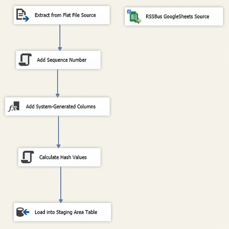
Loading the staging area follows a standard pattern because all incoming data items, such as flat files or relational tables, are sourced independently. To achieve this independence, there is no referential integrity implemented through foreign keys. Each staging table is a direct copy of the incoming data with only some system-generated attributes added. Figure 11.2 shows the template for loading a staging table.
Figure 11.2Template for staging area loading.
The first step is to truncate the staging tables, if only one load should be kept. If the staging area should follow best practices and keep a limited history, the truncation has to take place once the data has been loaded into the Raw Data Vault. For performance reason, it might be advisable to disable indexes on the staging area, if there are any implemented. The next step is to perform a bulk readon the source data from the source file or source database connection. As already mentioned, in order to achieve acceptable performance, the goal should be to read the data in chunks, not single records. If possible, complex APIs, such as the ones introduced by object-relational mapping (ORM), should be avoided. Instead, direct access to the relational tables or their raw data exported to flat files should be preferred. In Microsoft SQL Server, this can be achieved by executing the following T-SQL statement on the staging table [5]:
Another purpose of the staging area is to compute and add system-generated attributes to the incoming data. By doing this, reuse of the attributes is possible. Figure 11.3 shows the subprocess in more detail. In some cases, true duplicates exist in the source data. If they are kept and loaded into the Raw Data Vault, they would only create additional workload, but no additional changes to hubs and links. Depending on the implementation of the satellite loading processes, they could cause additional problems during change detection. This is why true duplicates should be removed from the staging area. Finally, the data is inserted into the staging table and indexes are rebuilt again. The Microsoft SQL Statement is very similar to the previous one [5]:
Figure 11.3Compute system values subprocess.
The following attributes are added in the Compute System Values subprocess, which is presented in Figure 11.3.
•Load date: the date and time when the batch arrived in the data warehouse (in the staging area). A batch includes all data that arrived as a set. In most cases, this includes all data in all flat files or relational tables from one source system.
•Record source: a readable string that identifies the source system and the module or source table where the data comes from. This is used for debugging purposes only and should help your team to trace errors.
•Sequence number: all records in a staging table are sequenced using a unique and ascending number. The purpose of this number is to recognize the order of the records in the source system and identify true duplicates, which are loaded to the staging area but not to downstream layers of the data warehouse. Note that the sequence number is not used for identification purposes of the record.
•Hash keys: every business key in the Raw Data Vault is hashed for identification purposes. This includes composite keys and key combinations used in Data Vault links. Chapter 4, Data Vault 2.0 Modeling, discusses how hash keys are used in hubs and links for identification purposes.
•Hash diffs: these keys are used to identify changes in descriptive attributes of satellite rows. This is also discussed in Chapter 4.
Because hash value computation consumes CPU power, there is an advantage of reusing the computed value. While the hash function that is used in this process is standardized (examples include MD5 and SHA-1), the input of the hash function has to follow organization-wide, defined standards. These standards have to be set by a governing body in the organization and should be based on the best practices as outlined in the next section.
11.2. Hashing in the Data Warehouse
Traditional data warehouse models often use sequence numbers to identify the records in other tables in the data warehouse and reference them in dependent tables. These numbers are generated in the data warehouse instead of being sourced from operational systems in order to use an independent sequence number that is controlled by the data warehouse.
There are multiple drawbacks with sequence numbers [6]:
•Dependencies in the loading processes: in order to load a destination, every dependency has to be loaded first. For example, loading a table that stores the customer addresses requires the loading of the customer table first, in order to look up the sequence number which identifies a particular customer.
•Waiting on caches for parent lookups: assuming sequence numbers instead of hashes would be applied. In this situation, Link and Satellite loads must “wait” for parent table lookup caches (particularly in ETL engines) to load with the cross-maps of business keys to sequence numbers. Hubs and links often contain large sets of rows that need to be cached before the ETL processing can begin. This causes a bottleneck in the loading processes. This can be alleviated or removed by switching the model to Data Vault 2.0 Hash Keys – eliminating the need for lookup caching altogether.
•Dependencies on serial algorithms: sequence numbers are often used as surrogate keys but they are what they are: sequences that are serial numbers. In order to generate such a sequence number, a sequence generator is often used, which presents a bottleneck because it needs to be synchronized in order to prevent two sequence numbers with the same value. In Big Data environments, the required synchronization can become a problem because data is coming at high speed and/or volume.
•Complete restore limitations: when restoring a parent table (e.g. the customer table from the previous example), the sequence numbers need to be the same as before the restore. Otherwise, the customer references in dependent tables become invalid (in the best case) or wrong (in the worst case).
•Required synchronization of multiple environments: if sequence numbers have to be unique across nodes or heterogeneous environments, synchronization of the sequence number generation is required. This synchronization can become a bottleneck in Big Data environments.
•Data distribution and partitioning in MPP environments: in MPP environments, the sequence number should not be used for data distribution or partitioning because queries can cause hot spots when getting data out of the MPP environment [7].
•Scalability issues: sequence numbers are easy to use but are limited when it comes to scalability. When using sequence numbers in large data warehouses with multiple terabytes or even petabytes of data, the sequence generation can become a bottleneck when loading large amounts of data. Sequences have an upper limit (usually), and in large data sets, or with repeated “restarts” due to error processing, the sequence generators can “run-out” of sequence numbers, and must then be cycled back to one. This is called roll-over, and isn’t a preferred situation – nor is it advisable to have this situation in a Big Data system to begin with. The other side of this situation is performance. With Big Data, many times the loading processes need to be run in parallel. Sequence generators, when “partitioned” so they can run in parallel, assign groups of sequences – and can hit the upper limits of the sequence number faster. Why? Each group of sequences (one per partitioned process) requires a block of sequences, and often leaves holes in the sequencing as it loads, thus eating up sequences much quicker than expected.
•Difference of NoSQL engines: in many cases, NoSQL engines use hash keys instead of sequence numbers because of the limitations regarding MPP data distribution and scalability, described in the previous bullet points.
Due to these drawbacks and limitations, hash keys are used as primary keys in the Data Vault 2.0 model, thus replacing sequence numbers as surrogate keys. Hash functions ensure that (exactly) the same input (on a bit level) produces the same hash value. The following sections discuss how to use this characteristic of hash functions for generating nonsequential surrogate keys that can be used in data warehousing.
Chapter 4 has outlined some benefits of using hash keys in the Data Vault 2.0 model: because hash keys are calculated independently in loading processes, there are no lookups into other Data Vault 2.0 entities required in order to get the surrogate key of a business key. In general, a lookup into another table requires I/O performance in order to retrieve the sequence number for a given business key. On the other hand, computing a hash key only requires CPU performance, which is often favored over I/O performance because of better parallelization and better resource consumption in general.
The alternative to hash keys is to use business keys as identifying elements in the data warehouse. However, using hash keys provides the advantage that the primary keys (and the referencing columns) can always use a fixed length data type, which has performance advantages in Microsoft SQL Server. This is due to the fixed-length column value that can be stored directly in the data page, requiring no lookups in additional database pages (text/image page) when performing table joins. Similar advantages are seen in other relational database management systems. While business keys in hubs might be shorter than hash keys, hash keys tend to be shorter in link tables (where multiple business keys are combined), a factor often overlooked when discussing the storage requirements of hash keys versus business keys.
But it’s not only the identification of business keys that can take advantage of introducing hash calculations in the data warehouse. Another advantage is the use of hash diff values, which can help to speed up column compares on descriptive attributes when loading satellites. This is of special interest for loading large amounts of raw data into satellites and is described in more detail in section 11.2.5.
While the benefits outweigh the drawbacks, the goal of the data warehouse is to reduce the number of hash key calculations in order to reduce CPU computations. Therefore, most hash values (hash keys and hash diffs) are calculated when loading the data from source systems into the stage area. This is not possible in every case, but is a desired strategy that should be achieved in 80% or more of the cases. Figure 11.4 shows potential locations in the loading process where hash values can be calculated if it is not possible to calculate and store the hash keys and hash diff values in the staging area.
Figure 11.4Stage load hash computation.
Calculating the hash values upstream to the data warehouse increases the reusability of the values in downstream processes towards the business user and prevents recomputation of the same hash key or hash diff value. On the other hand, the reusability of hash diff values is limited because they are only used in one satellite.
11.2.1. Hash Functions Revisited
There are multiple options available when applying hash functions in data warehousing. When selecting the hash function it is important to understand that hashing in the data warehouse doesn’t have any intention of encrypting or securing the business key. The only goal is to replace sequential surrogate keys by a hash key alternative [8]. Hash functions have a desired set of characteristics, including [8]:
•Deterministic: for a given block of input data, the hash function will always generate the same hash value whenever called.
•Irreversible: a hash function is an irreversible, one-way function. It is not possible to derive the source data from the hash value.
•Avalanche effect: if the input data is changed only slightly, the hash value should change drastically. Also known as a cascading effect.
•Collision-free: any two different blocks of input data should always produce different hash values. The unlikely event of two input blocks generating the same hash value is called a collision. These hash collisions is discussed in more detail in section 11.2.3.
The most common and recommended options for the purpose of hashing business keys include MD5 and SHA-1:
•MD5 message-digest algorithm (MD5): The MD5 algorithm was introduced in 1992 as a replacement of MD4. It takes a message of arbitrary length as an input and produces a 128-bit (16-byte) hash value, called a message digest or “signature” of the input. In cryptography, it was commonly used to digitally sign the input, such as an email message or file download to prevent later modifications [9].
•Secure hash algorithm (SHA): In 1995, SHA-1 was published as an industry standard for secure hash algorithms and should replace MD5 due to security concerns. SHA-1 is a U.S. Federal Information Processing Standard [10].
Table 11.1 shows some key statistics about the generated hashes of both algorithms and, with SHA-256, an implementation of the secure hash algorithm with a larger message digest size:
Table 11.1
Key Statistics for Selected Hash Algorithms
MD5
SHA-1
SHA-256
Max. Input Length
Unlimited
264-1 bits
264-1 bits
Output Length (binary)
128 bits (16 bytes)
160 bits (20 bytes)
256 bits (32 bytes)
Output Length (hex)
32 characters/bytes
40 characters/bytes
64 characters/bytes
The different output lengths are due to the fact that a character in hexadecimal representation can represent only 4 bits. For that reason, the space is doubled when using hexadecimal characters to represent the hash value. Section 11.2.2 discusses the advantages of the hexadecimal hash representation. Section 11.2.3 discusses the advantages of all three hash functions in more detail.
Note that both algorithms are used in cryptography, but they are not encryption algorithms. The hash result is typically encrypted with a private key, as used in public-key cryptosystems, for example RSA [11]. By doing so, a signature is created that is associated with the public key of the sender, which can be validated.
Unencrypted MD5 and SHA-1 hashes are often used to validate whether a download has not been compromised or accidentally modified due to transmission errors after downloading the file from the Web site of origin. For that reason, hashes are often seen next to downloads on Web sites, as shown in Figure 11.5.
Figure 11.5LibreOffice download with hash values for verification purposes.
In this case, there are multiple hash values provided using hexadecimal representation, including MD5, SHA-1 and SHA-256. By using hexadecimal characters, it is possible to include the hash value as a “readable” text directly into the Web site. Otherwise, the hash keys would have to be provided as additional binary file downloads. It is possible to validate the integrity of the downloaded file with a tool such as File Checksum Integrity Verifier (FCIV) from Microsoft [12]. The tool takes the downloaded file as input and reports the MD5 hash for the downloaded file:
If there is no difference between the bits of the file on the server and the bits of the downloaded file on the client, the output of the File Checksum Integrity Verifier should be the same as stated on the Web site in Figure 11.5.
11.2.2. Applying Hash Functions to Data
The approach described in the previous section uses an important characteristic of hash functions: the same input (on a bit level) produces the same, fixed-length hash value. In addition, the hash function produces a “random-like” value for each input. If only one bit changes in the input, the resulting hash value is not even close to the hash value without the changed bit. As described in the previous section, this characteristic is called the avalanche effect [13]. Consider the following examples:
Table 11.2 shows three example inputs and their respective MD5 and SHA-1 hash keys (note that MD5 outputs and SHA-1 outputs cannot be compared due to the different algorithms). Notice the inputs: the first two values are “Data Vault 2.0” and “DataVault 2.0”: a space between the first two words was removed. While this change seems to be minimal, it is actually not. The character length is different (from 14 characters down to 13) and therefore, the bit representation after the fourth character is completely different, as all following bits shift by eight characters to the left (Table 11.3).
Given their positions, all bold bits have changed, because they have been removed or shifted to the left. Therefore, we would expect this drastic change in the input to be reflected in their hash keys (which is the case in Table 11.2). And the same is true for an actual small change on the bit level (Table 11.4).
Here, only the first character case changes from an upper-case D to a lower-case d. Bitwise, the difference is just one bit that changes in the input, as indicated bold in Table 11.4: the bit on position 3 has changed from 0 to 1. However, even in this case of minor change, the hash values between example 2 and 3 in Table 11.2 are completely different, yet not randomly generated. The hash looks random, but it follows an algorithm that has the goal of ensuring that small changes have a high impact on the output – a desired characteristic in cryptography.
This characteristic is also desired when distributing the data in MPP environments such as Microsoft Analytics Platform System (formerly Microsoft SQL Server Parallel Data Warehouse). The distribution relies on a distribution column (other vendors call this a primary index). The data in this distribution column should be evenly distributed because all rows in a table are distributed according to this data in the column. If the data is skewed, the records will not be evenly distributed across the nodes, which will cause hot spots when answering queries [14]. Because the calculated hash value is “random-like,” it is a good candidate for a distribution column. Even similar data is distributed evenly on the nodes, thus ensuring that the maximum possible number of nodes answers queries.
Hash values can be calculated in a number of locations, for example directly in the database (using T-SQL functions), in SSIS, or in a third-party application. However, while the implementation of the hash algorithm should be the same (in the case of SHA-1, this can be ensured through a validation program by the NIST [15]), the resulting hash value depends heavily on the input to the function. Even the same sentence can produce different hash values if the input on the bit level is not exactly the same. Raw data types (integers, floats, etc.) make things worse, as the binary representation might differ from system to system. In order to calculate a re-usable hash value, that is a hash value that is the same for the same data input, all raw data types are converted into a string before hashing. That reduces the complexity of the approach to hash the data. The following requirements have to be met by the input string:
1.Character set: the character set defines how bits of a string or varchar are interpreted into readable characters. Or in other terms: how bits represent characters. Because commonly available hash functions work with bits instead of characters, the character set plays an important role to ensure that the same characters end up with the same bit representation. This includes Unicode vs. non-Unicode choices.
2.Leading and trailing spaces: in many cases, any leading and trailing spaces don’t play an important role for the business user of a data warehouse. For example, business keys usually don’t include leading or trailing spaces and descriptive data is often trimmed from them as well before presented to the user. Because they don’t change the meaning of the input and only the binary representation, they should not be included in the input to the hash function.
3.Embedded or unseen control characters: the same applies for any embedded or unseen control characters. Examples for this might be bell codes (BC) [16], carriage return (CR), new line (LF) or backspace sign, which often have no difference to the semantics of the text. Many of these control characters are inserted into text files or databases due to interoperability issues between operational systems.
4.Data type, length, precision and scale: the use of different data types, their length, and precision and scale settings produce different binary representations. For example, values stored in a decimal(5,2) or in a decimal(6,2) might be represented as the same characters, but are stored as different binary values. Therefore, one of the recommendations is to convert all data types to strings before hashing them.
5.Date format: when converting dates to strings, the question is how to represent dates in a common manner. It is recommended to cast all dates and timestamps into a standardized ISO8601 format [17].
6.Decimal separator: another problem when converting data types to strings concerns different regional settings. Depending on the current locale, different decimal and thousands separators are used. For example, the number 1,000.99 (in US format) is represented as 1.000,99 in Germany and 1’000.99 in Switzerland.
7.Case sensitivity: as already shown from the previous examples, the character case changes the binary representation of the string. Therefore, the character case has to be taken into consideration when hashing data. Depending on your data, case sensitivity needs to be turned on or off for your input data. For example, in most cases, business keys are case insensitive. Customer DE00042 is the same as de00042. There are exceptions to this rule, for example when business keys are actually case sensitive. The same applies to descriptive data that is often case sensitive, as well. We will discuss such examples in sections 11.2.4 and 11.2.5, respectively. Note that case sensitivity applies to the output as well. Some hash functions (or the accompanying conversion from binary values to a hexadecimal representation) produce a lower-case hex string, while others produce an upper-case hexadecimal string. The best practice is to convert all outputs from hash functions to upper-case.
8.NULL values: depending on the system where the hash value is calculated, the binary representation of a NULL value might be different, especially when converting NULL values to varchars or strings. Note that hash values are not always generated in a database but in other software environments such as the .NET framework, a Java Virtual Machine or in a Unix Shell. The recommended approach when dealing with NULL values is to always replace them by empty strings and use delimiters when concatenating multiple fields (for example, when calculating the hash key of a composite business key or the hash diff value of descriptive data).
9.Lack of delimiters for concatenated fields: because the recommendation is to replace NULL values by an empty string, there might be examples when different data becomes the same input after converting to strings and concatenating the individual elements of the input. Therefore the use of delimiters is required. This is described in more detail in section 11.2.4.
10.Order of concatenated fields: when concatenating fields, the order of the fields plays a vital role. If it is changed, the hash values become different.
11.Endianness: the architecture of software and hardware plays another significant role in how bytes are stored in memory. This can become an issue when not all hashes are generated on the same system, for example because some data is being hashed on other systems than the primary data warehouse system. For example, the .NET Framework is using little endian [18] (storing the least-significant byte (LSB) at the lowest memory address), while the Java Virtual Machine is using big endian [19] (storing the most significant byte (MSB) at the lowest memory address) as does Hadoop [20]. Microsoft SQL Server uses big endian in most cases [21]. On the hardware side, Intel® in its 80 × 86 architecture uses little endian [22].
12.Everything else: whenever the bit representation of the input string is changed, the hash value changes.
In order to deal with these issues and requirements, a first thought is to create a central function, such as a reusable user-defined function or SSIS script component that calculates the hash value by preparing the input and calling the appropriate hash function. However, this approach is often not enough, because today data is loaded into the data warehouse with various tools, for example an ETL tool such as SSIS, directly in the database (for example the stored procedure created in Chapter 10, Metadata Management) or in tools external to the data warehouse team. Other data is stored in NoSQL environments such as Hadoop and never touches the data warehouse until it is joined when building the information marts. However, if both parties use different approaches for dealing with these requirements, the join will fail, because the hash keys in hubs and links will be completely different from each other, preventing the joining of data across systems. For that reason, the first task when starting the data warehouse initiative is to create a standards document for hash value generation. The document should not only define which hashing function should be used to calculate the hash values, but also how the input is generated to ensure the same output for the same data. Table 11.5 reviews the standards that need to be established by this document and gives best practices for each.
Table 11.5
Best Practices for Hashing Standards Document
Standard
Best Practice
Hashing Function
MD5
Character set
UTF-8
Leading and trailing spaces
Strip
Control characters
Remove or change to blank (space)
Data type, length, precision and scale
Standardize to regional settings of organization’s headquarters
Date format
Standardize to regional settings of organization’s headquarters
Decimal separator
Standardize to regional settings of organization’s headquarters
Case sensitivity
Business keys: all upper-case; descriptive data: it depends
NULL values
Remove by changing to empty string or other default value
Delimiters for concatenated fields
Semicolon or comma
Endianness
Little Endian (due to SQL Server and the Java Virtual Machine which is used for Hadoop)
Note that the recommendation for Endianess and SQL Server is to use Little Endian because the HashBytes function appears to use Little Endian. Refer to section 11.6.3 for a discussion related to SQL Server and SSIS.
Addressing these requirements in the design phase and throughout the whole data warehouse lifecycle is the first step in dealing with technological risks regarding the use of hashes in data warehousing. However, there are additional risks, which are covered in the next section, that need to be mitigated.
11.2.3. Risks of Using Hash Functions
When using hash keys and hash diff values in the data warehouse, there are some additional issues that need to be considered in the design phase of the project. Ignoring these risks will sooner or later hit back on the data warehouse team.
11.2.3.1. Hash Collisions
Section 11.2.1 introduced collision freedom as a desired characteristic of hash functions. When hashing business keys while loading a hub, we want to prevent the hash function producing the same hash for two different business keys. Such a collision would represent a problem for a data warehouse built with Data Vault 2.0 modeling, because other entities, such as links or satellites, reference the business key using its hash value. If two business keys are using the same hash key, the reference would not be unique.
Because hash functions compress data from a theoretically unlimited input to a fixed-length hash value, it is not possible to prevent a hash collision, which is the same hash value for two arbitrary long inputs. And in fact, there are random inputs with the same hash key for any given meaningful input. For example, the 128-bit inputs (expressed in hexadecimal notation) shown in Table 11.6 produce the same MD5 hash value.
The common MD5 hash value is 008EE33A9D58B51CFEB425B0959121C9. This type of hash collision is called a general hash collision. It is not possible to prevent this problem if compression takes place. If all input is random, which means binary blocks of random input, there are various levels of risks, depending on the selected hash function. Figure 11.6 shows a comparison of risks (the odds of a hash collision) for CRC-32, MD5 and SHA-1.
Figure 11.6Probabilities of hash collisions [24].Figure adapted by author from “Hash Collision Probabilities,” by Jeff Preshing. Copyright Jeff Preshing. Reprinted with permission.
CRC-32 is not a recommended option for a hash function in data warehousing. However, it is included in Figure 11.6 to exemplify why this is the case: the risk of collisions is just too high. If a single hub or a single link contains only 77163 hashed records (a small-sized hub), the risk of a hash collision is 1 in 2 (50%). Using MD5, at least 5.06 billion (5.06 × 10⁹) records need to be included in the hub to get such a risk for collisions. Compare this to SHA-1: in order to reach a risk of 50%, the number of 1.42 × 1024 records have to be added into the same hub first. Note that if a collision happens in another Data Vault entity (two different inputs, the same hash value, but different hubs), the collision is not a problem at all because no data is referenced erroneously. Does it mean that there is no risk of hash collisions when only a small number of records to be hashed is involved? No. The risk is just negligible: if a hub contains only ∼200 business keys, hashed with MD5, the risk that a meteor would hit your data center is higher than that of a collision. The problem is that there is still a minor risk involved.
It is possible to reduce the risk even further by using the SHA-1 hash function. However, SHA-1 might not be available in all tools used in the data warehousing infrastructure. In these cases, the hashing function might be coded manually if that is possible.
However, for data warehousing purposes, the inputs for potential collisions are not random nor binary as in Table 11.6. Instead, they are meaningful: business keys follow a (limited) string format; even descriptive data in satellites has only a limited input to be meaningful. Therefore, the chance for a collision between two meaningful inputs is even lower as presented in Figure 11.6.
In reality, while the risk of a hash collision tends to be very low for MD5 and SHA-1, there is no way to guarantee that there will be no collisions in the operational lifetime of the data warehouse. But it is possible to check for the direct opposite: when designing the data warehouse, it is possible to check if there is already a collision in the initial load. By hashing all business keys of a source file, we can find out if there are already collisions using a given hash function (such as MD5). If that is the case, we can move to a hash function (such as SHA-1) with a larger hash value output (bit-wise) before making the choice of hash function permanently. But having no hash collisions in the initial load has no meaning for the future. The first collision could still occur on the first operational day, by chance.
While it is not possible to prevent collisions, it is possible to detect them at least. When loading hub tables, we can ensure that there is no other business key in the hub having the same hash key. The same applies to link tables where we check for existing business key combinations with the same hash key. It will slow down the loading patterns a little, but ensure that no data becomes corrupted in the data warehouse. There are also techniques to detect a hash diff collision, but the chances for such collision are very low, much lower than on hash keys in hubs and links. Both techniques are described in full detail in Chapter 12, Loading the Data Vault.
11.2.3.2. Storage Requirements
Another consideration includes the required additional storage to keep the hash keys and hash diffs. Using SHA-1 instead of MD5 increases the storage requirements from 32 bytes (MD5 in hexadecimal representation) to 40 bytes (SHA-1). Compare this to a big-integer sequence number that only requires 8 bytes.
Generally, the additional storage requirements are not a real problem in the enterprise data warehouse layer (modeled in Data Vault 2.0 notation). In our experience, the advantages (such as the loading performance) outweigh this disadvantage of consuming more storage.
However, most data warehouse teams prefer (big) integer surrogate keys in information marts, for two reasons: first, business users have direct access to the information mart and might be confused by hash keys in dimension and fact tables. In addition, the storage requirements for using hash keys in fact tables are a concern for many teams. Because fact tables usually refer to multiple dimension tables and contain many rows, the additional storage requirement of a hash key becomes an issue. Consider the example of a fact table that refers to 10 dimension tables. Each fact requires 320 bytes for referencing the 10 dimensions if MD5 is used. If the fact table contains 10 million rows, around 3 GB are required to store only the references. Using SHA-1 requires 3.8 GB for storing the references to the dimension tables. Compare this to 762 MB when using 8-byte integers. If you decide to avoid MD5 in favor of a SHA algorithm, it is recommended to use SHA-1 over SHA-256 (or higher) because of storage requirements. SHA-1 already provides superior resistance against collisions, which makes SHA-256 in most if not all cases irrelevant.
For that reason, information marts are typically modeled using sequence number instead of hash keys (refer to Chapter 7, Dimensional Modeling, for a detailed description).
When storing hashes, avoid using the varchar datatype. Columns that use a varchar datatype might be stored in text pages instead of the main data page under some circumstances. Microsoft SQL Server moves columns with variable length out of the data page if the row size grows over 8,060 bytes [26]. Because hash keys are used for joining, the join performance will greatly benefit from having the hash key in the data page. If the hash key is stored in the text page, it has to be de-referenced first. Columns using a fixed-length datatype are guaranteed to be included in the data page.
On some occasions, data warehouse teams try to save storage by using binary(16) for MD5 hashes or binary(20) for SHA-1 hashes. Doing so limits the interoperability with other systems, such as Hadoop or BizTalk. Therefore, this is not a recommended practice. If you decide to do it anyway, avoid using the varbinary datatype for the same reasons as avoiding the varchar datatype. More interoperability issues are discussed in the next section.
11.2.3.3. Tool and Platform Compatibility
One of the reasons why hash keys have been introduced is that they improve the interoperability between different platforms, such as the relational database and NoSQL environments. By using hash keys in hubs and links, it is possible to integrate data on various platforms, structured in the relational database and unstructured data in NoSQL environments such as Hadoop. For that reason, the recommended data type to store hash keys is varchar because it is easy to read and write by external applications. If other datatypes are used, an on-the-fly conversion might be required which slows down the read/write process and makes it more complex.
Compatibility with other tools and platforms is also the reason to recommend MD5 for hash keys. Many systems, such as ETL tools, are capable of calculating MD5 hash keys. While SHA-1 is the newer algorithm and the recommended hashing function for encryption purposes nowadays, not all tools typically used in the business intelligence domain support it. On the other hand, most ETL tools and database systems support the MD5 hashing function out of the box. For the same reason, it is not recommended to use MD6 (the direct successor of MD5), SHA-256 or any other hashing algorithm that doesn’t have widespread support compared to MD5 or SHA-1.
Before making a decision regarding the choice of hash function, the available tools and their hashing capabilities should be carefully reviewed to avoid surprises in later phases of the project.
11.2.3.4. Maintenance
In the rare case that a collision has occurred, the resolution includes increasing the bit-size of the hash value (hash key or hash diff) by changing the hash function. For example, if MD5 was used when a collision occurred, the recommendation is to move to SHA-1. This upgrade requires increasing the length of the hash key column (for example from 32 characters to 40) and to recalculate the hash values based on the business keys in the hub or link or the descriptive data in the satellites. Consider the recalculation of a hub’s hash keys. Because other links and satellites reference these hash keys in order to reference the hub (for example to describe the business key in a satellite), at a minimum, all hash keys in dependent entities have to be recalculated, as well. Theoretically, all other hash keys could be left at the smaller size.
But leaving some hash keys in the smaller hash size would increase the maintenance costs because more management is required. It also hinders any automation efforts or requires more complex metadata to accomplish this task. Therefore, the recommendation is to use only one hash function for calculating all the hashes in the data warehouse.
For the same reason, it should be avoided to use different hash algorithms in the relational data warehouse and unstructured NoSQL environments, such as Hadoop (Figure 11.7).
Figure 11.7 shows that both environments independently calculate hashes for the data stored in both worlds because the data is sourced independently. Both systems identify business keys and their relationships for the purpose of hashing. In addition, whole documents in Hadoop can be linked to the data warehouse by a Data Vault 2.0 link that references the hash key of the Hadoop document. It is also possible to join across both systems when building the information marts.
In order to make this approach work, make sure that all systems use the same hash function and the same approach to apply it to the input data (refer to section 11.2.2 for details).
11.2.3.5. Performance
From a theoretical standpoint, it requires more CPU power to calculate one hash value than to generate one sequence value. The previous chapters have already discussed the reason why hash values are favored over sequence values (with regards to performance):
•Easy to distribute hash key calculation: the hash key calculation depends only on the availability of the hash function (which might be a tool problem) and the business key that needs to be hashed. For that reason, the hashing can be distributed very easily, for example to other environments or to multiple cluster nodes.
•Hash key calculation is CPU not I/O intensive: calculating the hash key is a CPU intensive operation (consider the calculation of a large number of hash keys) but doesn’t require much I/O (the only I/O workload required is when storing the hash keys in the stage area for reusability). Because CPU workload can be easily and cheaply distributed over multiple CPUs, it is generally favored over I/O workload.
•Loading of dependent tables doesn’t require lookups: the biggest performance gain comes from the fact that calculating the hash key requires only the business key, as described in the first bullet point. This advantage makes the lookup to retrieve the business key’s sequence number from a hub obsolete. Because lookups cost a high amount of I/O, this is a popular advantage with high performance benefits.
•Reduce the need for column comparing: another intensive operation in data warehousing is to detect a change in descriptive data for versioning. In Data Vault, this happens when loading new rows into satellites because only deltas are stored in satellites. In order to detect if the new row should be stored in the satellite (which requires that at least one column be changed in the source system), every column between the source system (in the staging table) and the satellite has to be compared for a change. It also requires dealing with possible NULL values. Hash diff values can reduce the necessary comparisons to only one comparison: the hash diff value itself. Section 11.2.5 will show how to take advantage of the hash diff value.
In summary, hash keys provide a huge performance gain in most cases, especially when dealing with large amounts of data. For these reasons (and the additional ones regarding the integration with other environments), sequence numbers have been replaced by hash keys in Data Vault 2.0.
The previous sections have shown some advantages of hash functions in data warehousing, but they are no silver bullets [26]. Depending on how they are used, new problems might be introduced that need to be dealt with. However, the advantages of hash keys outweigh their drawbacks.
11.2.4. Hashing Business Keys
The purpose of hash keys is to provide a surrogate key for business keys, composite business keys and business key combinations. Hash keys are defined in parent tables, which are hubs and links in Data Vault 2.0. They are used by all dependent Data Vault 2.0 structures, including links, satellites, bridges and PIT tables. Consider a hub example from Chapter 4 (Figure 11.8).
Figure 11.8Hub with hash key (physical design).
The hash key FlightHashKey is used for identification purposes of the business keys Carrier and FlightNum in the hub. All other attributes are metadata columns that are described later in this chapter. For link structures, the hash key that is used as an identifying element of the link is based on the business keys from the referenced hubs (Figure 11.9).
Figure 11.9Link with hash keys (physical design).
Note that there are a total of five hash keys in the LinkConnection link. Four of them are referencing other hubs. Only the ConnectionHashKey element is used as the primary key. This key is not calculated from the four hash values, but from the business keys they are actually based on. When loading the link structure, these business keys are usually available to the loading process.
Calculating a hash from other hash values is not recommended because it requires cascading hash operations. In order to calculate a hash based on other hashes, these hashes have to be calculated in the link loading process first. Because this operation might involve multiple layers of hashes, many unnecessary hash operations are introduced. Because they are CPU intensive operations, the primary goal of the loading patterns is to reduce them as much as possible.
In order to calculate hash key for hubs and links, it is required to concatenate all business key columns (think about composite business keys) and apply the guidelines from section 11.2.2 before the hash function is applied to the input. The following pseudo code shows the operation with n individual business keys in the composite key of the hub:
BKi represents the individual business key in the composite key and d the chosen delimiter. The order of the business keys should follow the definition of the physical table and should be part of the documentation. If the business key is not a composite business key, n equals to 1 and the above function is applied without delimiters. It assumes that all other standards, especially the endianness and character set, are taken care of. This also includes any control characters in the business keys and common conversion rules for various data types, for example floating values or dates and timestamps.
The approach is the same for hubs and links: in the case of links, each BKi represents a business key from the referenced hubs (see Figure 11.10). If hubs with composite business keys are used, all individual parts of the composite business key are included. For degenerated links, all degenerated fields have to be included as well. These weak hub references are part of the identifying hash key as any other hub reference.
Figure 11.10Satellite with multiple hub references (physical design).
While not intended on purpose, some of the individual business keys might be NULL. Because most database systems return NULL from string concatenations if one of the operators is a NULL value, NULL values have to be replaced by empty strings. Without the delimiter, the meaning of the business key combination would change in an erroneous way. Consider the example rows in Table 11.7.
Table 11.7
Importance of Delimiters
BK 1
BK 2
BK 3
BK 4
Hash Result (without Delimiters)
Hash Result (with Delimiters)
Row 1
ABC
(null)
DEF
GHI
6FEB8AC01A4400A7 28B482D0506C4BEB
D9D33F7E6E80D174 7C45465025E9E6AF
Row 2
ABC
DEF
(null)
GHI
6FEB8AC01A4400A7 28B482D0506C4BEB
FD4D58C47B5C343A 4A9E23922ABE4C46
After concatenating the four business keys without a delimiter, the string becomes in both cases “ABCDEFGHI”. Because the input to the hash function is the same, the resulting hash value is the same as well. But it is obvious that both rows are different and should produce different hash values. This is achieved by using a semicolon (or any other character sequence) as a delimiter. The first row is concatenated to “ABC;;DEF;GHI” and the second row to “ABC;DEF;;GHI”. After sending the data through the hashing function, the desired output is achieved by retrieving different hash values.
In the previous chapter, a statement similar to the following T-SQL statement was used to perform the operation:
This statement implements the previous pseudocode using Microsoft’s MD5 implementation in SQL Server 2014 and takes care of potential NULL values in addition. Note that each individual business key (the variables, such as @event, in the above statement) is checked for NULL values using the COALESCE function. The business keys are also removed from leading and trailing spaces on an individual basis. In this example, a semicolon is used to separate the business keys before they are being hashed using the HASHBYTES function. The result of this function is a varbinary value. This varbinary is converted to a char(32) value. The last UPPER function around the CONVERT function makes sure that the hexadecimal hash key is using only uppercase letters. If SHA-1 should be used instead, the result from the HASHBYTES function has to be converted to a char(40) instead.
Note that, in rare cases, business keys are case-sensitive. In this case, the upper case function has to be avoided in order to generate a valid hash key that is able to distinguish between the different cases. Keep in mind that the goal is to differentiate between the different semantics of each key, not to follow the rules at all cost.
It is also possible to implement this approach in ETL, for example by using a SSIS community component SSIS Multiple Hash[27] or using a Script Component (standard component in SSIS). The latter is demonstrated in section 11.6.3.
11.2.5. Hashing for Change Detection
Hash functions can also be used to detect changes in descriptive attributes. As described in Chapter 4, descriptive attributes are loaded from the source systems to Data Vault 2.0 satellites. Satellites are delta-driven and store incoming records only when at least one of the source columns has changed. In this case, the whole (new) record is loaded to a new record in the satellite. The loading process of satellites (and other entities) is discussed in the next chapter.
In order to detect a change that requires an insert into the target satellite, the columns of the source system have to be compared with the current record in the target satellite. If any of the column values differ, a change is detected and the record is loaded into the target. To perform the change detection, every column in the source must be compared with its equivalent column in the target. Especially when loading large amounts of data, this process can become too slow in some cases. For such cases, there is an alternative that involves hash values on the column values to be compared. Instead of comparing each individual column values, only two hash values (the hash diffs) are compared, which can improve the performance of the change detection process and therefore the satellite loading process.
The basic idea of the hash diff is the same as the hash key in the previous section: it uses the fact that, given a specific input, the hash function will always return the same hash value. Instead of comparing individual columns, only the hash diff on these columns is used (Table 11.8).
Table 11.8
Example Data Compared by Hash Diff (without a Change)
Attribute Name
Stage Table Value
Satellite Table Value
Title
Mrs.
Mrs.
First Name
Amy
Amy
Last Name
Miller
Miller
Hash Diff
CADAB1708BF002A85C49FF78DCFD9A65
CADAB1708BF002A85C49FF78DCFD9A65
Table 11.8 shows data in a stage table and the current record in the target satellite. Both records are hashed using a MD5 hash function, which results in a 32-character-long hash diff. Because the descriptive data is the same in the stage table as in the satellite table, both sides share the same hash diff value. After comparing the hash diff column (instead of the individual columns title, first name and last name) no change is detected and, as a result, no row is inserted into the satellite. If the data changes only a little, the hash diff value becomes different (Table 11.9).
Table 11.9
Example Data Compared by Hash Diff (with Change)
Attribute Name
Stage Table Value
Satellite Table Value
Title
Mrs.
Mrs.
First Name
Amy
Amy
Last Name
Freeman
Miller
Hash Diff
66C17DF4D91EE9F0CF39490BFCC20B60
CADAB1708BF002A85C49FF78DCFD9A65
As a result of the changed data, the hash diff is completely different. Because of this different value, it is easy to detect changes in the stage table without comparing the values itself. While both hash diffs have to be calculated, the hash from the satellite can be reused whenever data is loaded, because it is stored with the descriptive data in the satellite, as Figure 11.10 shows.
The satellite SatAirport contains a number of descriptive attributes. The HashDiff attribute stores the hash diff over the descriptive attributes and can be reused whenever a record in the stage table is present that describes the parent airport (identified by AirportHashKey).
The hash diff is calculated in a similar manner to the hash keys in the previous section. All descriptive attributes are concatenated using a delimiter before the hash diff is calculated. Before concatenating the attributes, leading and trailing spaces are removed and the data is formatted in a standardized format. Especially the data type, date formats, and decimal separators are of importance, because all descriptive data, including dates, decimal values and all other data types have to be converted to strings before the data is hashed. The following pseudocode is used within the first, yet incomplete, approach:
Datai indicates descriptive attributes, d a delimiter. The only difference between the pseudocode in this section and the previous section (to calculate hash keys on business keys) is that the upper case function has been removed: in many cases, change detection should trigger a new satellite entry if the case of a character is changing. However, this depends on the requirements given by the organization. In other cases, case-sensitive descriptive data is set on a per-satellite basis or even a per-attribute basis. How case-sensitivity is implemented depends on the definition of the source system and the data warehouse, as well.
The above pseudocode is not complete yet. In order to increase the uniqueness among different parent values, the business keys of the parent are added to the hash diff function. Consider the example shown in Table 11.10.
Table 11.10
Different Parents with the Same Descriptive Data
Passenger HashKey
LoadDate
LoadEndDate
Record Source
Title
First Name
Last Name
9d4ef8a…
2014-06-03
9999-12-31
DomesticFlight
Mrs.
Amy
Miller
12af89e…
2014-06-05
9999-12-31
DomesticFlight
Mrs.
Amy
Miller
In this case, there are two passengers Mrs. Amy Miller. They are distinguished by different hash keys, which result from different inputs, the business keys. If only the descriptive data is included in the hash diff calculation, both records would share the same hash diff value. This might not be very dangerous, but if the hash diffs were different, yet correct, we could use the hash diff to find a specific version of the descriptive data for one individual parent without using a combination of both the parent hash key and the hash diff. It is desired to have a hash diff that is unique over all satellite records, because then it would be sufficient to use only the hash diff to locate a particular version, which might improve the query performance for loading patterns in some circumstances.
We achieve this uniqueness of the hash key by adding the business keys of the parent to the hash diff calculation:
The business keys of the parent are just added in front of the descriptive data, delimited by the same delimiter and following the same guidelines as outlined in the previous section. Both groups, the business keys and the descriptive data, must follow a documented order. A good practice is to use the column order of the table definition. In many cases, the business keys are uppercased while descriptive data remains case sensitive. Keep this in mind when standardizing and developing the hash diff function. Note that it’s not the hash that is added to the front of the descriptive data but the business keys themselves. This follows the recommendation to avoid hashing hashes (hash-a-hash) in order to avoid cascaded calculations (refer to the previous section for more details).
The input to the hash function for the examples in Table 11.10 is presented in Table 11.11.
Table 11.11
Example Input to Hash Diff Function
Input to Hash Function
Hash Diff
7878;Mrs.;Amy;Miller
9DA0891434B92DF529B8CCCD86CC140B
2323;Mrs.;Amy;Miller
E890EE7980D5B13449704293A1BB4CCA
Because the input to the hash function is different (due to the included business key), the hash value for both inputs is different. When loading the satellites, it is ensured that this hash diff can be regained at any time because both the descriptive data as well as the business keys are available. Therefore, this is the recommended practice.
11.2.5.1. Maintaining the Hash Diffs
Using the hash diff can improve the performance of the satellite loading processes, especially on tables with many columns. However, it incurs a maintenance cost or effort in addition to the calculation in the stage area. The reason for this additional maintenance is that satellite tables might change. Consider the following example, presented in Table 11.12 to Table 11.14, which adds a column academic title to the example provided previously:
Table 11.12
Initial Satellite Structure
Passenger HashKey
LoadDate
LoadEndDate
Record Source
Title
First Name
Last Name
8473d2a…
1991-06-26
9999-12-31
DomesticFlight
Mrs.
Amy
Miller
9d8e72a…
2001-06-03
9999-12-31
DomesticFlight
Mr.
Peter
Heinz
Table 11.13
Satellite Structure After Adding a New Column
Passenger HashKey
LoadDate
LoadEndDate
Record Source
Title
Academic Title
First Name
Last Name
8473d2a…
1991-06-26
9999-12-31
DomesticFlight
Mrs.
(null)
Amy
Miller
9d8e72a…
2001-06-03
9999-12-31
DomesticFlight
Mr.
(null)
Peter
Heinz
Table 11.14
New Records are being Added to the New Satellite Structure
Passenger HashKey
LoadDate
LoadEndDate
Record Source
Title
Academic Title
First Name
Last Name
8473d2a…
1991-06-26
2003-03-03
DomesticFlight
Mrs.
(null)
Amy
Miller
9d8e72a…
2001-06-03
9999-12-31
DomesticFlight
Mr.
(null)
Peter
Heinz
8473d2a…
2014-06-20
9999-12-31
DomesticFlight
Mrs.
Dr.
Amy
Freeman
The first table shows the old satellite structure, with three descriptive attributes, namely title, first name and last name. Because the source system has changed, a new descriptive attribute is added in Table 11.13, called academic title. Because the source systems never delivered any data for this new column in the past, it is set to NULL, or any other value representing this fact.
Once the new column has been added to the source table, it can capture incoming data. In this case, a new record is being added to the table that overrides the first record (Amy Miller marries Mr. Freeman). In addition, the source system provides an academic title for Mrs. Freeman. It is unclear if she always held this title, but from a data warehousing perspective, it makes no difference. For audit reasons, the old records will not be updated because at the time when they have been loaded (indicated by the load date), the source system did not deliver an academic title for her (or any other record).
The issue arises when hash diffs are used in this satellite. Tables 11.15,11.16 and 11.17 show the hash diffs for the above examples (in the same order as previously).
Table 11.15
Hash Diffs for Initial Satellite Structure
Passenger HashKey
LoadDate
LoadEndDate
Hash Diff
8473d2a… {4455}
1991-06-26
9999-12-31
BDD9DD9208611F2A8CF3670053634FF0
9d8e72a… {6677}
2001-06-03
9999-12-31
B3B1724EF449DA9D9521FA95A88A82A3
Table 11.16
Hash Diffs for Satellite Structure After Adding a New Column
Passenger HashKey
LoadDate
LoadEndDate
Hash Diff
8473d2a… {4455}
1991-06-26
9999-12-31
4F860465EB585FABF3CBD28E7A29AEC0
9d8e72a… {6677}
2001-06-03
9999-12-31
FFCF6191C583F5B77273D4CABF3EB98F
Table 11.17
Hash Diffs After New Records Have Been Added to the New Satellite Structure
Passenger HashKey
LoadDate
LoadEndDate
Hash Diff
8473d2a… {4455}
1991-06-26
2003-03-03
4F860465EB585FABF3CBD28E7A29AEC0
9d8e72a… {6677}
2001-06-03
9999-12-31
FFCF6191C583F5B77273D4CABF3EB98F
8473d2a… {4455}
2014-06-20
9999-12-31
1C1E8C1799E39E567F746F720800B0E5
The numbers in the curly brackets indicate the corresponding business keys. The first table shows the MD5 values for the descriptive data. Note that the hash diffs are different to the ones provided in Table 11 because the example was slightly different: other business keys were used in that example.
The semantic meaning of the data behind the hash diffs in Table 11.15 and Table 11.16 did not change (compare this to Table 11.12 and Table 11.13). However, the hash diffs changed, indicating to the change detection that the rows have changed. The only difference between these tables is the introduction of a new column, academic title. But the new column has changed everything because it influenced the input to the hash diff function (Table 11.18).
Table 11.18
Modified Example Input to Hash Diff Function
Input to Hash Function
Hash Diff
4455;Mrs.;Amy;Miller
BDD9DD9208611F2A8CF3670053634FF0
4455;Mrs.;;Amy;Miller
4F860465EB585FABF3CBD28E7A29AEC0
The first row presents the input for Amy Miller before the structural change to the satellite, and the second row the input after the column has been added. Notice the added semicolon in the input on the left side, between the title and the first name. This semicolon is due to the fact that a NULL column was introduced and changed to an empty string. The advantage of the semicolon that it allows for NULL values now becomes a disadvantage.
However, we actually need the new hash diff value because, otherwise, we’re unable to detect any changes in the source system. If we leave the old hash diffs in the satellite table, all current source records (modified or unmodified) are interpreted as modified, due to the different hash diff value. Therefore, we need to update all hash diffs in the satellite table to prevent unnecessary (and unwanted) inserts into the satellite table.
It is possible to avoid this maintenance overhead of the hash diff by following a simple strategy. The first idea is to update only the current records in the satellite. They are indicated by having no load end date (or in the examples of this book, an end-date of 9999-12-31), because only those records are required for any regular comparison during satellite loading. All end-dated satellite entries have been replaced by newer records already and are not required to compare with. This approach reduces the number of records to be updated after structural changes but still incurs many updates, especially when there are many different parent entries.
But it is actually possible to further reduce the maintenance overhead to zero: by making sure that the hash diffs remain valid, even after structural changes. However, there are some conditions to make this happen:
1. Columns are only added, not deleted.
2. All new columns are added at the end of the table.
3. Columns that are NULL and at the end of the table are not added to the input of the hash function.
The first condition is required because of auditability reasons in any case. The goal of the data warehouse is to provide all data that was sourced at a given time. If columns are deleted, the auditability is not achieved anymore.
Meeting the second and the third condition is best explained by an example (Table 11.19, modified from Table 11.18):
Table 11.19
Improving the Hash Diff Calculation
Input to Hash Function
Hash Diff
4455;Mrs.;Amy;Miller
BDD9DD9208611F2A8CF3670053634FF0
4455;Mrs.;Amy;Miller;
D64074FE047165874481A7B299C4A766
4455;Mrs.;Amy;Miller
BDD9DD9208611F2A8CF3670053634FF0
The first line shows the input to the hash function before the structural change. The second line shows the input after the structural change, meeting the first two conditions, but not the third. Instead of adding the new column in the middle between the title and the first name, the academic title is added at the end of the table. Without meeting the last condition, a semicolon is added and the NULL value is added after the semicolon as an empty string. Because the input has changed by the addition of the semicolon character, the hash diff has changed, indicating a change.
If the third condition is met in addition, all empty columns at the end of the input are removed before the hash function is called. It means that all trailing semicolons are being removed. That way, the input becomes the same again and the hash diffs indicate no change because they have to be the same. This approach works with multiple NULL columns at the end.
How does it improve the satellite loading process? First, the old hash diffs are still valid. There is no semantic difference between the rows in Table 11.19. The only difference is a structural change that should not have an impact on the satellite loading process by triggering an insert operation into the satellite. This is achieved by this improved hash diff calculation.
However, if a new column is added to the satellite and the source system provides a value for the new column, a new hash diff is being calculated (Table 11.20).
Table 11.20
Changing the Semantic Meaning
Input to Hash Function
Hash Diff
4455;Mrs.;Amy;Miller
BDD9DD9208611F2A8CF3670053634FF0
4455;Mrs.;Amy;Miller;Dr.
0044E798C5586E931A604D1E0CD09FA1
Because the input to the hash function has changed between the two loads, the hash function will return two different hash diffs. This is in line with the requirements of the satellite loading process because the satellite should capture the change in Table 11.20.
The biggest advantage of the presented approach is that the hash diff values are always valid if the conditions listed earlier are met. On the other hand, the disadvantage is that the satellite columns might be in a different order than the source table, for example when new columns are added to the source table after it was initially sourced into the data warehouse. However, because this approach doesn’t affect the auditability at all, we recommend this approach in most cases.
11.3. Purpose of the Load Date
The load date identifies “the date and time at which the data is physically inserted directly into the database”[6]. In the case of the data warehouse, this might be the staging area, the Raw Data Vault or any other area where the data arrives. Once the data has arrived in the data warehouse, the load date is set and is part of the auditable metadata. Except for satellites, the load date is primarily a metadata attribute that helps when debugging the data warehouse. However, because it is part of the satellite’s primary key, it is in fact an essential part of the model that needs to be taken special care of.
If the database system that is used for the data warehouse supports it, the load date should represent the instant that the data is inserted to the database. The time of arrival should be accurately identified down to a millisecond level in order to support potential real-time ingestion of data. If the database system doesn’t support timestamps but only dates, the alternative is to add a sub-sequence number to the load date that represents pseudo millisecond counters. This is required for satellites in order to make the primary key (which consists of the parent hash key and the load date) unique. This uniqueness requires milliseconds because data might be delivered multiple times a day (in batches or in real time).
The data warehouse has to be in control of the load date. Again, this is especially important for the Data Vault satellites because the load date is included in the satellite’s primary key. If the load date breaks for any reason, the model will break and stop the loading process of the data warehouse. A load date typically breaks if two different batches are identified by the same load date. In this case, the satellite loading process would try to insert records (due to a detected change) with a duplicate key. For example, if a create date or export date from the source system that is not controlled by the data warehouse is used as a load date, the following issues are implicated:
•Mixed arrival latency: not all data arrives at the same batch window timeframe. There is often some form of ongoing mixed arrival schedule for source data. When the load date is generated during the insert into the data warehouse, this mixed arrival date time can be assigned gracefully. The inserts to the Raw Data Vault (in this case) occur at the time of arrival. In one case, the business needs to be updated every 5 seconds with live feed data; in another case, the EDW needs to show a time-lineage of arrival to an auditor for traceability reasons.
•Mixed time zones for source data: not all data is being created in the same time zone. Some source systems are located in the USA, some in India, and so on. If a create date were to be used as a load date, these time zones have to be aligned on the way into the data warehouse. Any conversion, no matter how simple, slows down the loading process of the data warehouse and increases the complexity. Increased complexity will not only increase the maintenance effort but also the chance that errors happen.
•Missing dates on sources: not all source systems provide a create date or another candidate to be used as a load date. Dealing with these exceptions requires conditions in the loading procedures, which should be avoided because it adds complexity again. Instead, apply the same logic to all sources to keep the loading procedures as simple as possible.
•Trustworthiness of dates on sources: not all source systems run correctly. In some cases, the time of the source system has an offset due to a wrong configuration or hardware failures (consider a defunct motherboard battery). In other cases, the date and time configuration of the source system is changed between loads (for example to fix an erroneous configuration or after replacing the motherboard battery). This actually makes things worse as it complicates the matters when times now overlap.
If the data warehouse team decides to use an external timestamp as the load date, the data warehouse loading process will fail in the following scenarios:
•Create date is modified by source system: the data warehouse team has no control over the create date from the external system. If the source system owner or the source system application decides to change the create date for any reason, it has to be handled by the data warehouse. However, how should this change be handled if the load date is part of the immutable primary key within satellites? Changing it is not possible for auditing reasons.
•Loading history with create date as load date: in other cases, the data warehouse team has to source historical data that might or might not have create dates. For example, if the source system has introduced the create date in a later version, historical data from earlier versions don’t provide the create date.
For all these reasons, the load date has to be created by the data warehouse and not sourced from an external system. This also ensures the auditability of the data warehouse system because it allows auditors to reconcile the raw data warehouse data to the source systems. The load date further helps to analyze errors by loading cycles or inspecting the arrival of data in the data warehouse. It is also possible to analyze the actual latency between time of creation and time of arrival in the data warehouse.
System-driven load dates (system-driven by the data warehouse) can be used to determine the most recent / most current data set available for release downstream to the business users. While it doesn’t provide complete temporal information, it provides the technical view on the most recent raw data or at any given point in time.
But what should be done with the dates and timestamps from the source system? Typically, the following timelines exist in source systems:
• Data creation dates
• Data modified dates
• Data extract dates
• Data applied dates such as
• Effective start and end dates
• Built dates
• Scheduled dates
• Executed dates
• Deleted dates
• Planned dates
• Financed dates
• Cancelled dates
None of these dates or any other date from the source system qualify as load dates. However, they provide value to the business. As such, they should be included in the data warehouse as descriptive data and loaded to Data Vault satellites.
11.4. Purpose of the Record Source
The record source has been added for debugging purposes only. It can and should be used by the data warehousing team to trace where the row data came from. In order to achieve this, the record source is a string attribute that provides a technical name of the source system, as detailed as it is required. In most cases, data warehouse teams decide to use some hierarchical structure to indicate not only the source system, but also the module or table name. If accessing a relational Microsoft SQL Server source, the record source should use the following format:
For example, the following record source would indicate a table from the CRM application, in the Cust schema:
Avoid using only the name of the source system because following this approach can be very helpful when tracing down errors. When analyzing the data warehouse due to a run-time error, either in development or production, it is helpful to have detailed information available.
The record source is added to all tables in the staging area, the Raw Data Vault, the Business Vault and probably the information marts. But what if data from multiple sources is combined or aggregated? In this case, the record source is not clear anymore. The recommended practice is to set the record source to the technical name of the business rule that generated the record. The technical name can be found in the metadata of the data warehouse (refer to Chapter 10, Metadata Management). If there is no business rule, the record source should be set to SYSTEM. Examples include the ghost record in satellites (see Chapter 6, Advanced Data Vault Modeling) or any other system-driven records.
Use of record sources that are dependent on a specific load should be avoided. For example, the file name is often not a good candidate for a record source, especially if it contains a date. The record source should group all data together that comes from the same origin of data. Having a date in the record source prevents this. The same applies for physical database or server names: what if the location of the data changes? The file name, the database name or the server name might be changed in the future, even if the source where the records came from remains the same.
11.5. Types of Data Sources
The data warehouse can source the raw data from a variety of data sources, including structured, semi-structured and unstructured sources. Data can also come from operational systems in batch loads or in real time, through the Enterprise Service Bus (ESB). Typical examples for source systems in data warehousing include [28]:
•Relational tables: operational systems often work with a relational database backend, such as Microsoft SQL Server, Oracle, MySQL, PostgreSQL, etc. This data can be directly accessed using OLE DB or ADO.NET sources in SSIS [29].
•Text files: if direct access of the relational database is not permitted, operational systems often export data into text files, such as comma-separated files (CSV) or files with fixed-length fields [29].
•XML documents: in other cases, operational systems also provide XML files that can be processed in SSIS [29].
•JSON documents: similar to XML documents, JSON documents provide semi-structured files that can be processed by SSIS using additional third-party components.
•Spreadsheets: a lot of business data is stored in spreadsheets, such as Microsoft Excel files, which can be directly sourced from SSIS [29] and Google Sheets, which can be sourced with third-party components.
•CRM systems: customer data is often stored in customer relationship management (CRM) systems, such as Microsoft Dynamics CRM, Salesforce CRM or SAP. Third-party data sources allow sourcing this data.
•ERP systems: organizations use ERP systems to store data from business activities, such as product planning, manufacturing, marketing and sales, inventory management or shipping and payment. Examples for ERP systems include Microsoft Dynamics ERP, Microsoft Dynamics GP, SAP ERP, and NetSuite. There are third-party data sources available for sourcing data from ERP systems.
•CMS systems: content management systems (CMS) provide the ability to create intranet applications for unstructured or semi-structured content. Third-party connectors allow connecting to CMS systems such as Microsoft SharePoint.
•Accounting software: this type of software is used to manage general ledger and perform other financial activities, such as payroll management. Examples include QuickBooks and Xero. Third-party components allow sourcing of data from these systems.
•Unstructured documents: include Word documents, PowerPoint presentations and other unstructured documents.
•Semi-structured documents: include emails, EDI messages, and OFX financial data formats which can be sourced with third-party components.
•Cloud databases: more and more data is stored in the cloud, for example in Microsoft Azure SQL Database, Amazon SimpleDB, or Amazon DynamoDB. Microsoft Azure SQL Database is supported by the OLE DB data source; other cloud databases are supported by third-party vendors.
•Web sources: the Internet provides a rich set of third-party data that can be added to the data warehouse in order to enrich the data from operational systems. The same applies to data from Intranet locations. Examples for file formats used typically in such settings include RSS feeds (for news syndication), OData and JSON (for standardized access to data sets) in addition to general XML documents. Some of these formats can be sourced by SSIS with built-in capabilities. Others require a third-party data driver.
•Social networks: social networks present another, yet more advanced, Web source. There are SSIS data sources to process data from social networks such as Twitter and Facebook.
•Mainframe copybooks: a lot of operational data is managed by mainframe systems and will be in the future. EBCDIC files are one of the standards and can be handled by SSIS with additional components.
•File systems: not all documents are stored in local file systems. Instead, some data resides on FTP servers, can be copied using secure copy (SCP) commands or is in the cloud, for example Amazon S3. Third-party components can assist in retrieving data from such remote stores.
•Remote terminals: In other cases, the data is on remote servers, but only accessible via remote terminals, such as telnet or secure shell (SSH). Again, third-party vendors extend SSIS if that is required.
•Network access: even TCP ports on the network might provide data that is sourced into the data warehouse.
In order to load the data using ETL tools, the access methods have to be supported by the tool itself. Not all tools support all data sources, but it is possible to extend them by custom components. Microsoft SSIS is such an example where the base functionality can be extended by custom components from third-party vendors. It is also possible to add generic data sources from the Web, especially by accessing REST or XML Web Services. Additional SSIS components can be found on CodePlex [30].
The remaining sections discuss how to source typical data sources, including the sample airline data that is used throughout the book.
11.6. Sourcing Flat Files
The first example loads flat files into the data warehouse. These flat files are typically exported from operational systems, which often use a relational database. Flat files include several of the previously listed formats, including comma-separated files (CSV), fixed-length files and Microsoft Excel Sheets.
When sourcing text-based files, such as CSV or fixed-length files, all data is formatted as strings. In order to convert the raw data during the export in the source system, which also uses other data types, such as integers, or decimal values, a format is applied to build the string text that is exported into the text file. By doing so, the source application defines, for example for decimal values, how many positions after the decimal point should be included and how many should be rounded off.
11.6.1. Control Flow
The companion Web site provides three CSV files from the BTS database, introduced in the opening of this chapter. In order to run the following example in SSIS, you have to extract the Zip file and place the CSV files into one folder. The final SSIS control flow will traverse through the folder and load all data from all CSV files in the folder into the staging area.
In order to traverse through the folder, drag a Foreach Loop Container on the canvas of the control flow. Double-click to edit it and set the following parameters as shown in Figure 11.11.
Figure 11.11Configuring the collection of the foreach loop container.
Change the Enumerator type to Foreach File Enumerator. Configure the file enumerator by setting the Folder to the location where the CSV files from the companion Web site are located. Change the Files wildcard to *.csv and Retrieve file name to Name and extension.
The last option defines how the file name of the traversed file should be stored in a variable. It is possible to store:
• the name and extension: only the file name and the file extension are stored in the variable.
• the fully qualified name: this includes the file location and the file name including the extension of the file.
• the name only: only the file name, without the file extension, is stored.
Select the option to store the fully qualified name because the full name is required by the data flow that will be created in the next step.
The variable that stores the file name of the currently traversed file is set on the next tab Variable Mappings (Figure 11.12).
Figure 11.12Map variable of foreach loop container.
To store the file name in a variable, either choose a pre-existing variable or create a new variable by focusing the cell in the Variable column of the grid and selecting <New Variable…>. The dialog as shown in Figure 11.13 will appear.
Figure 11.13Add variable to store file name from foreach loop container.
Set the container of the variable to package. For the purpose of this example, it would also be sufficient to set it to the foreach loop container itself to reduce the scope of the variable. Set the name of the variable to sFileName. We will later reference the variable using this variable name. The namespace should be set to User or a defined namespace of your choice that is used to store such variables. Set the value type to String, as it will store the file name and extension of the traversed file. The default value should be set to default or something similar. Make sure read only is not selected.
After selecting the OK button, the variable is added to the previous variable mapping dialog and shown in the table with index 0 (Figure 11.14).
Figure 11.14Added variable to the foreach loop container.
Confirm the foreach loop editor by selecting OK. The next task ensures a consistent load date over all records in each file. For this purpose, the current timestamp is set to a SSIS variable using a Microsoft Visual C# script: whenever the container loops over a file, it first sets the current timestamp into the variable User::dLoadDate and then starts the data flow, which is discussed next. The data flow will use the timestamp in the variable to set the load date in the staging area. Follow the earlier approach and create a new SSIS variable by selecting the Variables menu entry in the context menu of the control flow. Create a new variable with name dLoadDate and the settings as shown in Table 11.21.
Table 11.21
Variable dLoadDate Settings
Parameter
Value
Name
dLoadDate
Scope
Package
Data type
DateTime
Value
12/30/1899
Close the dialog and drag a Script Task into the container. Open the editor as shown in Figure 11.15.
Figure 11.15Script task editor to set the load date.
Add the variable User::dLoadDate to the ReadWriteVariables by using the dialog available after pressing the button with the … caption. Check the variable in the dialog and close it. Edit the script and enter the following code in the Main function:
This code writes the current timestamp of the system into the variable and reports a successful completion of the function to SSIS.
Add a Data Flow Task to the container and rename it to Stage BTS On Time On Time Performance. The final control flow is presented in Figure 11.16.
Figure 11.16Control flow to source flat files.
The foreach loop container will enumerate over all files in the configured folder. Sort order of the file names appears to be in alphabetic order, but this is undocumented by Microsoft. There are custom components that allow sorting by file name and date among other options [31].
The next step is to configure the data flow task in order to stage the data in the flat files into the target tables.
11.6.2. Flat File Connection Manager
In order to set up the data flow for staging CSV flat files, the first step is to set up the flat file connection manager. Open the Stage BTS On Time On Time Performance data flow in the previous SSIS control flow. Drag a Flat File Source to the data flow (Figure 11.17).
Figure 11.17Flat file source editor.
Create a new flat file connection by selecting the New… button. In the following Flat File Connection Manager Editor, select one of the flat files in the source folder (Figure 11.18).
Figure 11.18Setting up the flat file connection.
Make sure the locale is set to English (United States) and Unicode is not selected. The format should be set to Delimited, double quotes (“) should be used as text qualifier and header row delimiter is set to {CR}{LF} as usual under Microsoft Windows. The column names are provided in the first data row of the source file; therefore activate the corresponding check box.
The data from the source file can be previewed on the columns tab. Switch to the advanced tab to configure the data types and other characteristics of the columns (Figure 11.19).
Figure 11.19Configure columns of the flat file connection.
This configuration is required because the CSV file doesn’t provide any metadata or description of the data, except the column headers. All data is formatted as strings only. While it is possible to manually configure the columns, it is also possible to use a wizard that analyzes the source data. Select the Suggest Types… button to start the wizard in Figure 11.20 (Figure 11.20).
Figure 11.20Suggest column types configuration.
The wizard analyzevs the source data by looking at a sample size only. This sample size should be large enough to capture all types of different characteristics of the data. Turn on the first two options and identify Boolean columns by 1 and 0. This follows the recommendation to use the actual data types of the raw data. Columns such as delayed are Boolean fields, which are formatted as 0 and 1. Make sure that pad string columns is turned off. After selecting the OK button, review the definitions of the source columns in the previous dialog. Note that some of the columns might have been incorrectly classified as Boolean because the data contains only records from January, which is in quarter 1 and month 1. Change them to better data types, such as two-byte signed integer. Also, you should increase some of the output column width of the string columns to allow longer city names, for example. Change all string columns from strings to Unicode strings. More information about the source columns can be found in the readme.html file that accompanies the source files.
After completion of the flat file connection manager editor, select retain null values from the source as null values in the data flow in the flat file source editor. Close the editor by selecting the OK button.
So far, the filename in the Flat File Connection Manager was configured using a static file name. This allows easy configuration of the columns and previewing data. In order to successfully traverse over all files in the source folder, we need to change the file name programmatically. Select the Flat File Connection Manager in the Connection Managers pane at the bottom of Microsoft Visual Studio and set the DelayValidation property to True. Open the expressions editor by clicking the ellipse button. The dialog in Figure 11.21 is shown.
Figure 11.21Property expression editor for flat file connection manager.
Set the ConnectionString property by the following expression: @[User::sFileName]. This will set the file name to the file name stored in the SSIS variable obtained in the control flow.
11.6.3. Data Flow
After having configured the flat file connection, the next step is to add the system-generated attributes in the control flow and load the data into the destination.
The following system-generated attributes should be added to the stage table:
•Sequence number: a number that is used to maintain the order of the source file in the relational database table.
•Record source: the source of origin of the data.
•Load date: the date and time when the record was loaded into the data warehouse. This should be consistent for all records in one file but different to other files.
•Hash keys: surrogate keys for each business key and their relations, based on a hash function.
•Hash diffs: hash values used to speed up column comparisons when loading descriptive data.
The primary key of the staging table consists of the sequence number and the load date. The combination of both fields must be unique for this reason.
The first step is to add the sequence number to the data flow. Microsoft SSIS doesn’t provide a sequence generator. If the sequence should be created within SSIS, a Script Component is used. An alternative is to create an IDENTITY column in the Microsoft SQL Server table. The script component allows fully customized transformations, written in C# or Visual Basic.NET, to extend SSIS. Drag the component to the data flow canvas. The dialog in Figure 11.22 will be shown.
Figure 11.22Select script component type.
It is possible to use the script component in three different ways:
•Source: the script component acts as a source and sends records into the data flow. This is useful when loading data from data sources not directly supported by SSIS.
•Destination: the script component acts as a destination and supports writing records from the data flow into third-party locations such as custom APIs.
•Transformation: the script component transforms the input records from the data flow into different outputs and writes them back to the data flow.
Because the goal of this step is to attach a sequence number to the data flow, select transformation before pressing the OK button. Connect the data flow of the flat file source to the script component. Open the Script Transformation Editor and add a new column on the Inputs and Outputs tab (Figure 11.23).
Figure 11.23Script transformation editor to create a sequence output.
Select the folder Output Columns of the first output called Output 0. Select the Add Column button below the tree view. Name the output column Sequence and set the DataType property to four-byte signed integer [DT_I4]. Switch back to the Script tab and select the Edit Script… button on the bottom right of the dialog. Replace the Input0_ProcessInputRow function by the following code:
This code introduces a new seq field that is increased for each row and returned into the data flow. Close the script and the script transformation editor.
The next step is to add the record source and the load date. Adding them is fairly simple: a Derived Column component can be added to the data flow. This is due to the simplicity of the required calculations. Drag a Derived Column component on the data flow canvas and connect it to the previous script component. Add the derived columns as shown in Table 11.22.
Table 11.22
Derived Columns Required for Staging Process
Derived Column Name
Expression
Data Type
LoadDate
@[User::dLoadDate]
date
RecordSource
“BTS.OnTimeOnTimePerformance”
Unicode string
The first derived column creates a LoadDate column in the data flow. This column retrieves the load date from the variable, which was set in the control flow before the data flow was started. The RecordSource column is set statically to a detailed string that can be used for debugging purposes.
In addition, the same component can be used to prepare the hash calculations. For each hub and link in the target Data Vault model as shown in Figure 11.1, a hash key is required that is based on the business key or business key relationship in the model. There are five hubs and two links in the model. But the source file provides multiple columns that are mapped to the same target entity. For example, both origin and destination airports are mapped to the HubAirport. For that reason, multiple columns have to be hashed. Add the derived columns as shown in Table 11.23, which will represent the various inputs for the hash function.
Table 11.23
Additional Derived Columns Required for Hashing in the Staging Process
Note that some of the input columns are converted to Unicode strings by the expression (DT_WSTR,X) where X is the configured length of the output string. All elements in the business key (BK) or the satellite payload (PL) for descriptive data are checked for NULL values by using the REPLACENULL function. Note the combination of case-insensitive business keys and case-sensitive payload in the last two derived columns.
The delimiter is hard-coded into the derived column because it can only be changed later with much effort. Changing the delimiter from semicolon to another character requires full reloading of the data warehouse. Also, it might be required to improve the expressions to support additional data types (such as Boolean and float values) and to standardize on the date format to be used: it is recommended to use ISO-8601 for converting date timestamps into character strings.
The Div1FlightLinkBK to Div5FlightLinkBK columns include a constant value that helps to un-pivot the incoming data. If the flight was diverted multiple times, the diversion information is provided in up to five sets of columns. When loading the data into the Raw Data Vault, it is loaded into a single link table with up to five records per incoming row.
Figure 11.24Derived column transformation editor to setup the system-generated columns.
The new columns are shown in the grid on the bottom of the dialog. Select OK to close the dialog. The next step is to calculate the hash values for all business keys, their relationships and for descriptive attributes that should be added to the same satellites. Multiple options have been discussed in section 11.2. This section describes how to use a Script Component for hashing the inputs.
Drag another Script Component to the data flow canvas and connect it to the previous Derived Column transformation. Switch to the Input Columns tab and check all available input columns in the default input Input 0. Switch to the Inputs and Outputs tab. For each derived column that ends with HubBK, LinkBK or SatPL, add a corresponding HashKey or HashDiff column. For example, for FlightNumHubBK, add an output column FlightNumHashKey with a string (non-unicode) of length 32 and code page 1252. Because the hash value is based only on characters from 0 to 9 and A to F, a Western European code page, such as 1252 or even ASCII, is sufficient. The important step here is to define the one to be used and implement it consistently.
Following this naming convention is important for the following script to work, because it hashes all input columns ending with either HubBK, LinkBK or SatPL and writes them into an output column with exactly the same name, ending with HashKey or HashDiff instead. This approach requires no programming at all; all configuration is done graphically in the Script Transformation Editor (Figure 11.25).
Figure 11.25Output columns in the script transformation editor for applying the hash function.
Switch back to the Script tab and enter the following script using the Edit Script… button:
This script traverses through all input columns, checks if their names end with either HubBK, LinkBK or SatPL, replaces these suffixes with HashKey or HashDiff and applies the MD5 hash function before storing the hash value in the output column. In order to make this script compile successfully, a reference to the assembly System.Security is required.
Note that this script implements a simplified hash diff calculation. It has not implemented the improved strategy to support changing satellite structures as described in section 11.2.5 with zero maintenance. In order to do so, any delimiters at the end of the input strings for hash diffs (columns ending with “SatPL”) have to be removed from the input.
The last step is to set up the OLE DB destination to write the data flow into a staging table. Before doing so, create the target table in the staging area by executing the following script:
In this script, all strings are configured as nvarchar to allow other languages to be added later on. It is also in line with the flat file source in the data flow, because the input columns have been configured as Unicode strings. The table is created in a schema called bts. The schemas as used in this chapter follow the convention that each source system uses its own schema.
The final step is to set up the destination. Drag an OLE DB Destination component to the data flow canvas and connect it to the Script Component that calculates the hash values. In the OLE DB Destination Editor, create a new connection manager. Set up the new connection to the StageArea database as shown in Figure 11.26.
Figure 11.26Setup connection manager.
After selecting the OK button, make sure the connection is taken over to the OLE DB destination editor and select the OnTimeOnTimePerformance table in the bts namespace as the destination (Figure 11.27).
Figure 11.27Set up OLE DB destination.
Make sure to keep null values by activating the option. You might want to configure the other options, such as rows per batch. Switch to the Mappings tab and make sure that all columns from the data flow are mapped correctly to the destination (Figure 11.28).
Figure 11.28Map input columns to destination.
Scroll down and make sure that the HubBK, LinkBK and SatPL columns have not found a destination column. They are only used in the data flow but not written to the destination. Instead, the corresponding hash key or hash diff value is written.
Run the control flow by pressing the start button in the toolbar. After moving the data, open Microsoft SQL Server Management Studio and execute the following SQL statement to compare the hash calculation in TSQL with the one performed in SSIS:
The statement should return four columns. The first two columns should return the OriginHashKey and provide exactly the same result. The last two columns should produce the same OriginAirportHashDiff value.
Note that there are two options to convert the columnValue variable in line 32 of the script used in the script component to calculate the hash values. This option is set in line 5 when the System.Text.UnicodeEncoding class is initialized:
The first parameter in the constructor allows to set little endian (false) or big endian (true) for the conversion. When using big endian, the hash values produced in SSIS are different from those produced in T-SQL. Also make sure that the byte-order mark (the second parameter is set to false).
The control and data flows to source flat files into the staging area are now complete. Note that the Metrics Mart and Error Mart have been left out of the discussion by intention, due to space restrictions. In order to go productive, redirect errors into the Error Mart as shown in Chapter 10, Metadata Management, and capture base metrics in the same manner as discussed in Chapter 10 as well.
11.7. Sourcing Historical Data
The previous section described the loading of flat file data sources. However, one special case remains that needs some thought. Before the data warehouse is put into production and loads data on a regular schedule, historical data is often loaded. The historical data often comes from the source application itself, from the archive or from a legacy data warehouse. Sourcing historical data allows the business to analyze trends that have started before the data warehouse has been put in place. Therefore, loading historical data is a common task in data warehousing.
Section 11.3 has described how the load date is applied to incoming data in order to identify the batch that loaded the data. When using this approach without modifications for loading historical data, a problem is incorporated into the loading process. Because all historical data is loaded in one batch, or at least in multiple batches around the same time, there is a risk that historical data cannot be loaded into the Data Vault any longer. If the same load date is used for all historical data, it would actually become impossible to load the data. The reason behind this problem is that the load date is part of the Data Vault 2.0 model because it is included in the primary key of satellites. Consider the three historical source files in Figure 11.29.
Figure 11.29Historical source files generated on various dates.
All three files contain address data for the same passenger. The passenger has moved over time. Because this historical data is of interest for the business users, it needs to be loaded into the data warehouse before going into production. If the initial data load, based on the historical data, is performed on January 1, 2015, the load dates for all three documents would be set to this date. Consider the effects on the satellite SatPassengerAddress shown in Table 11.24.
Table 11.24
Erroneous SatPassengerAddress Satellite
Passenger HashKey
Load Date
Load End Date
Record
Source
Address
City
Zip
State
Country
8473d2a…
2015-01-01 08:34:12
2015-01-01 08:34:12.999
Domestic Flight
31 Main St.
Norman
30782
OK
USA
8473d2a…
2015-01-01
08:34:12
2015-01-01 08:34:12.999
Domestic Flight
9612 Lincoln Road
Santa Clara
70831
CA
USA
8473d2a…
2015-01-01 08:34:12
9999-12-31 24:59:59.999
Domestic Flight
2050 1st street
San Francisco
94114
CA
USA
The problem is that the load date in Table 11.24 has been set to the same date. In fact, loading this data into the satellite table will not work, because the primary key is made up of the passenger hash key column and the load date column (refer to Chapter 4). This combination has to be unique to meet the requirements of the primary key. These records would be in violation with these requirements because the combination is always the same for all three rows.
To resolve this issue, there are two options: either load the data in three different batches, or set an artificial load date. The first solution would work from a technical perspective, but from a design perspective, there should be no difference between historical data and actual data. The data warehouse should pretend that the historical data was loaded just as the actual data on the day it was generated (or at least near the date). In the case of the example shown in Table 11.24, all historical data seems to be loaded on January 1, 2015. This is true, but not the desired view of the business.
The second approach is to set the load date to an artificial date. This is the preferred solution when loading archived historical data. The load date is set to the date it would have received if the historical data had been loaded in the past. By doing so, it simulates that the data warehouse would have been in place and the loading procedures would have sourced the file in the past. This is the only exception to the rule that the load date should not be a source-system generated date, because we’re using the date of generation, in many cases the extract date. On the other hand, this is a one-off historical load and the load date is only derived from the historical date of generation, but under full control of the data warehouse. For example, the data warehouse team might decide to override a load date derived from the historic date of generation during the initial node when required. For all these reasons, the date of generation could be used as the load date (Table 11.25).
Table 11.25
Corrected Satellite Data for SatPassengerAddress
Passenger HashKey
Load Date
Load End Date
Record
Source
Address
City
Zip
State
Country
8473d2a…
1995-06-26 00:00:00.000
2000-05-20 23:59:59.999
Domestic Flight
31 Main St.
Norman
30782
OK
USA
8473d2a…
2000-05-20 00:00:00.000
2007-04-21 23:59:59.999
Domestic Flight
9612 Lincoln Road
Santa Clara
70831
CA
USA
8473d2a…
2007-04-21 00:00:00.000
9999-12-31 23:59:59.999
Domestic Flight
2050 1st street
San Francisco
94114
CA
USA
Note that the time part of the load date has been set to 00:00:00.000. There are two reasons for this decision: first, in many cases, the actual time when the historical data has been extracted from the source system is unknown because the file name or some log file provides only the date of extraction. The second reason is that the convention to set the time part of the load date for historical data helps to distinguish the historical data from the actual data which is still desired in some cases, for example for debugging purposes. Following this recommendation is a compromise between the ability to distinguish the data from each other and the desire to load the historical data as it would have been loaded in the past.
11.7.1. SSIS Example for Sourcing Historical Data
Because the load date is set in the staging area, it has to be overridden in its loading processes when historical data should be loaded. In section 11.6, the current date was set as the load date by writing the timestamp into a SSIS variable using a script task. This script task needs to be modified for loading historical data. The goal is to develop a SSIS package that is able to handle both types of data (historical data for the initial load and daily loads).
The first step is to allow read-only access to the current file name in the forloop container. Open the Script Task Editor and select the ellipsis button to modify the ReadOnlyVariables (Figure 11.30).
Figure 11.30Script task editor to add ReadOnlyVariables.
In the following dialog, add the Users::sFileName variable which holds the current file name of the container that traverses over all files in the source directory.
The second step is to modify the source code of the script task. Instead of setting the current date, the following source is used to extract the date of extraction from the filename:
The year, month and day are extracted from the source file name using a regular expression that captures dates from file names with YYYY_MM_DD formatted dates included in the file name. These expressions search for patterns within strings and are useful to extract information from semi-structured text such as the file names. If an error occurs, the error is reported to the Error Mart.
11.8. Sourcing the Sample Airline Data
The BTS data is provided as Google Sheets on Google Drive. The folder is accessible by the general public under the following link: http://goo.gl/TQ1R63. We will load the data from the Google Sheet files into the staging area of the local data warehouse.
Microsoft SSIS does not provide a component for easy access to files on Google Drive. However, it is possible to extend SSIS by Google Sheets components that can directly access live Google Sheets. In order to do so, download the following products from CData.com:
•CData ADO.NET Provider for Google Apps: The CData ADO.NET Provider for Google Apps gives developers the power to easily connect .NET applications to popular Google Services including Google Docs, Google Calendar, Google Talk, Search, and more. We will use the components to load all Google Sheets from the public folder on Google Drive [32]. The product can be found here: http://www.cdata.com/drivers/google/ado/
•CData SSIS Components for Google Spreadsheets: Powerful SSIS Source & Destination Components that allows you to easily connect SQL Server with live Google Spreadsheets through SSIS Workflows. We will use the Google Spreadsheets Data Flow Components to source the airline data from Google Sheets [33]. The product can be downloaded from http://www.cdata.com/drivers/gsheets/ssis/
The vendor provides an extended free trial for the purpose of this book. Use the given trial subscription codes when installing the software on your development machine (Table 11.26).
Table 11.26
License Keys for CData Components Required to Download the Sample Data
Product Name: CData SSIS Components for Google Spreadsheets 2015 [RLSAA]License: EVALUATION COPY
Product Key: XRLSA-ASPST-D4FFD-2841W-MRREM
Product Name: CData ADO.NET Provider for Google Apps 2015 [RGRAA]
License: EVALUATION COPY
Product Key: XRGRA-AS1SR-V4FFD-2851T-ZWAFZ
Note: If you decide to buy the components for your projects, you can use the coupon code DVAULT10 to receive a 10% discount on the software.
As an alternative, you can also download the files as zipped CSV files manually from Google Drive, store them unpacked in a local folder and load the files using the procedure described in the previous section.
The next sections describe how to traverse over Google Drive in order to find the location and name of the airline data spreadsheets. It then sources each spreadsheet into the staging area. Before doing so, access to the Google Drive account has to be granted using OAuth 2.0. Otherwise traversing files on Google Drive is not allowed due to security concerns.
11.8.1. Authenticating with Google Drive
Before the control flow is modified in the next section, Google Drive has to be set up in order to provide the data to SSIS. This requires two steps:
1. Import the folder under http://goo.gl/TQ1R63 into your personal Google Drive account.
2. Allow SSIS to connect to your Google Drive account by registering it as a Desktop application.
Provide a unique project name and project id. Select Create to create the project in your account. Wait until the project has been created. Once the project dashboard shows up, configure the consent screen by selecting the corresponding menu item under APIs & auth (Figure 11.32).
Figure 11.32Setup Consent screen.
The consent screen is presented to the end-user in order to grant access to the personal Google Drive account. No worries: this user will just be you and nobody else.
Enter some information that identifies the application to the user and select the Save button.
OAuth 2.0 authorization is required to access the entities on Google Drive that we need to access in order to traverse all the airline data spreadsheets. Without it, the SSIS job described in the next sections cannot find out which spreadsheets are available. Therefore, select the Create new Client ID button to advance to the next screen (Figure 11.33).
Figure 11.33Create client ID for desktop application.
Depending on the application type, different mechanisms are used to authenticate the application to the user. There are different settings for Web applications, service accounts and applications installed on local desktops or handheld devices. From a cloud provider point-of-view, SSIS is an installed desktop application. Therefore, select the Installed application option and Other as the application type. Create the client ID by pressing the default button on the screen. The client ID will be created and presented to you (Figure 11.34).
Figure 11.34Client ID for native application.
The first items, the client ID and the client secret, are required to allow your local SSIS control flow to access your Google Drive account. Write down both pieces of information or keep your Web browser open. Also, make sure to keep this information secret. When entering the information in the control or data flow, the consent screen will be opened in the default Web browser. When that happens, log into your Google account and confirm the application.
Lastly, make sure to enable the Drive API and the Drive SDK under APIs.
11.8.2. Control Flow
The first step is to find out the Google Spreadsheets that are available on the Google Drive account. The basic idea is to use the ADO.NET provider for Google Apps to search for all spreadsheets with a name similar to “On_Time_On_Time” by performing a SELECT operation against the provider.
Drag an Execute SQL Task to the control flow, outside of the existing Foreach Loop Container (Figure 11.35).
Figure 11.35Execute SQL task editor for the Google Drive connection.
Set the ConnectionType property to ADO.NET and create a new connection (Figure 11.36).
Figure 11.36Connection manager for the Google Drive connection.
Set the properties as shown in Table 11.27 for the connection.
Table 11.27
Property Values for the Google Drive Connection
Property
Value
Initiate OAuth
True
OAuth Settings Location
A folder on the local file system accessible by SSIS
OAuth Client Id
Your client ID created in the previous section
OAuth Client Secret
Your client secret created in the previous section
Pseudo Columns
*=*
Readonly
True
Timeout
0
The first four properties are related to the authentication process. Note that there is also another authentication method available, based on user and password credentials. However, Google requires OAuth 2.0 for the operations performed by this SSIS control flow.
The pseudo columns setting activates all pseudo columns in all tables. The pseudo columns are required in order to perform a search on Google Drive. This is discussed next. Set timeout to 0 in order to avoid SSIS errors due to timeouts when selecting a large number of Google Spreadsheets.
Once the connection has been set up completely, select the OK button and finish the configuration of the Execute SQL Task: set the ResultSet property to Full Result Set and enter the following query in the SQLStatement property:
The statement selects the title and the spreadsheet ID of those files from Google Drive that meet the following conditions:
1. The title starts with “On_Time_On_Time”: this makes sure that only files are selected that provide airline data.
2. The file is not trashed.
3. The file is a Google Spreadsheet.
4. The file is starred (optional).
The last condition reduces the number of spreadsheets returned by this query to a manageable number of documents: it only returns spreadsheets that have been starred. Remove this WHERE condition to retrieve all spreadsheets for the airline data. If you leave this option in, make sure you have actually starred some of the airline spreadsheets.
The conditions are provided to Google Drive by a pseudo column called Query. This pseudo column doesn’t exist in the source sheet but is used by the CData ADO.NET source for Google Apps to provide the query in a SQL friendly format. Additional search parameters can be found under the following URL: https://developers.google.com/drive/web/search-parameters.
Both the title and the feed link are required: the title is used to extract the load date as described in section 11.7. The feed link is used to access the data from the spreadsheet in the data flow.
Because the ADO.NET provider returns one row per spreadsheet, the result set has to be stored in an object variable. This can be configured on the Result Set tab of the Execute SQL Task Editor (Figure 11.37).
Figure 11.37Configure the result set.
Create a new variable in the User namespace. Set the value type to Object because it will be used to store the whole dataset returned by the ADO.NET provider. Associate it to the result with name 0 as shown in Figure 11.37.
Close the editor and connect the Execute SQL Task to the Foreach Loop Container in the control flow (Figure 11.38).
Figure 11.38Control flow to source the sample airline data.
The next step is to change the foreach loop container because it should no longer traverse over the local file system. Instead, it should traverse over the ADO.NET result set stored in the object variable. Open the editor of the container and switch to the Collection tab (Figure 11.39).
Figure 11.39Modifying the enumerator of the foreach loop container.
Change the enumerator to a Foreach ADO Enumerator. Set the ADO object source variable to the one that was configured in Figure 11.38. Make sure that the enumeration mode is set to Rows in the first table. Switch to the Variable Mappings tab in order to map from the columns in the result set to SSIS variables that can be used in the control and data flow (Figure 11.40).
Figure 11.40Variable mappings to map the columns in the result set to variables.
The first column contains the title of the spreadsheet. This is the clear name that is also shown when viewing the Google Drive folder online. Make sure it is mapped to the sFileName variable created in section 11.6. The second column in the result set contains the feed link, which is required by the data flow to access the spreadsheet data. Create a new variable in the User namespace called sFeedLink with a value type of String and set the default value to a valid feed link, such as https://spreadsheets.google.com/feeds/worksheets/1gsbCxxTmfSZnoZQxCN1hoSZfnXFNgu-79JMwn35iVNc/private/full.
Setting this default value is required to configure the data flow properly. The feed link can be copied from the following Web site to avoid typing it in:
You should also set the sFileName variable to the name of the sheet within the spreadsheet behind the feed link to avoid issues in the data flow later. Therefore, set the default value to “On_Time_On_Time_Performance_2006_2_27_DL”.
Setting up the variables completes the setup of the control flow. The next step is to configure the data flow by changing the source.
11.8.3. GoogleSheets Connection Manager
After installation of both software packages, you will notice two new components in the SSIS Toolbox when switching to the Data Flow tab, as shown in Figure 11.41.
Figure 11.41SSIS Toolbox with CData components.
You can move the components into the Other Source or Other Destination folder by opening their context menu and selecting the respective menu item.
Drag a CData GoogleSheets Source to the data flow created in the previous section. It will replace the Flat File Source that was used before. Open the editor by double clicking the source and create a new connection using the New… button. The dialog shown in Figure 11.42 will appear.
Figure 11.42Connection manager to set up the Google Sheets connection.
Enter the information shown in Table 11.28 to set up the connection to a sample Google Sheets document.
Table 11.28
Required Property Values to Set Up the Google Sheets Connection
Property
Value
Initiate OAuth
True
OAuth Settings Location
A folder on the local file system accessible by SSIS. Make sure to use another folder than the one configured in the previous section.
The spreadsheet value should be set to the feed link that will be obtained in the control flow. It uniquely identifies a spreadsheet. For now, it is set as a constant value and replaced in an expression later. It is also possible to provide the name of the spreadsheet. However, because the API is limited to a small number of spreadsheets that can be accessed by name (there is an API limit that allows only 500 spreadsheet names to return), providing the feed link is a more secure way. To avoid typing in the feed link, copy it from the following Web site:
The property Detect Data Types should be turned off by setting its value to 0. In most cases, this option is quite useful, because it automatically detects the data types of the columns in the spreadsheet by analyzing a number of records. The number of records it uses for this analysis can be provided here. The more records it analyzes, the more secure the data type detection becomes [34]. However, because not all the airline data uploaded to Google Drive has diversions (the columns towards the right), the data type detection might fail. In order to avoid any such problems, we have decided to completely turn off the feature and force the source component to set all data types to varchar(2000) instead. This will affect the staging table as well.
Close the dialog by selecting the OK button. The connection is taken over as the active connection manager in the previous dialog. Because each spreadsheet has multiple tabs, select the corresponding tab from the Table or View box (Figure 11.43).
Figure 11.43Setting up the connection in the CData GoogleSheets source editor.
Select the table On_Time_On_Time_Performance_2006_2_27_DL from the list. The Spreadsheets view is a virtual view that returns a list of available spreadsheets (but it is limited to the 500 records). You can preview the data in the spreadsheet using the Preview button (Figure 11.44).
Figure 11.44Previewing the data from the spreadsheet.
Also, make sure that switching to the columns tab in the editor retrieves the columns in the source. Close the source editor.
11.8.4. Data Flow
The next step is to replace the flat file connection in the data flow by the Google Sheets Source (Figures 11.45 and 11.46).
Figure 11.45Data flow utilizing the flat file source.
Figure 11.46Data flow utilizing the Google spreadsheet.
Delete the old data flow path and connect the Google spreadsheet source to next component in the data flow (Add Sequence Number). After both components are connected, error messages are shown on two of the components.
The first error is on the script component that calculates the hash values. This is because the input column definition has changed and requires a rebuild of the script. Open the editor, open the script and rebuild it. After closing the script editor and the dialog, the error should be gone.
The second issue is a warning that indicates a column truncation. This warning appears because the destination table in the staging area is modeled after actual data types from the source file. Because the Google Sheets Source only provides strings, another staging table is required. Use the following T-SQL script to create a new staging table*:
Notice the nvarchar(2000) data types used for most columns (except the system-generated columns and the Id column that identifies each row in the Google Spreadsheets document). The alternative to convert all columns to the data types used in section 11.6.2 is too complicated in the staging process. Also, it would hinder automation efforts. Remember that another purpose for the staging area is to allow easy retrieval of the data from the source system. The data will be converted into the actual data types when it is loaded into the next layer, which is the Enterprise Data Warehouse (EDW) layer, modeled as a Data Vault 2.0 model.
Once the table has been created, it can be set as the target in the OLE DB Destination Editor (Figure 11.47).
Figure 11.47Configure OLE DB destination editor to use the new staging table.
Select the new staging table [bts].[OnTimeOnTimePerformanceGD] from the list of tables in the staging area. All other options should remain the same. However, make sure that the columns from the data flow are still mapped to the target columns because the name of the columns has changed. It follows the convention of the Google API to change the column name to lower-case, except the first letter. For example, the column name DestAirportID becomes Destairportid. Therefore, a remap of the columns is required. Change to the Mappings tab and select the Map Items by Matching Names menu item (Figure 11.48).
Figure 11.48Remapping the columns after changing the data source.
Make sure that all columns have been mapped. After selecting the OK button, start the process to load some data into the target table in the staging area. Generate and compare some of the hash values as described in section 11.6.3 to validate the process. If the hash values (either the hash keys or the hash diffs) are different, a problem has occurred in the SSIS process.
Finally, the configuration of the data flow needs to be adjusted in order to make use of the variables from the control flow. In the control flow, select the CData GoogleSheets Connection Manager and open the property expressions editor from its properties (Figure 11.49).
Figure 11.49Property expression editor for GoogleSheets connection manager.
Set the expression of the Spreadsheet property to @[User::sFeedLink].
Close the expression editor and set DelayValidation to True.
Select the canvas of the data flow and open the expression editor in its properties (Figure 11.50).
Figure 11.50Property expression editor for data flow task.
Select the property [CData GoogleSheets Source].[TableOrView] to dynamically set the name of the table (which is the sheet name within Google Sheets). Set it to the variable sFileName by adding the expression @[User::sFileName]. Confirm the dialog.
Finally, set the property ValidateExternalMetadata of the CData GoogleSheets Source to False in order to prevent validation of the variable at design-time.
To make this SSIS control flow less resource consuming (especially storage in the staging area), you could introduce command line parameters to the SSIS package and stage individual files, load them into the Raw Data Vault and truncate the staging tables before loading the next Google Sheet from the cloud. Using this approach, only one batch is staged during this initial load at a given time. However, it requires that the Raw Data Vault be loaded just after staging an individual file. This is covered in the next chapter.
11.9. Sourcing Denormalized Data Sources
In some cases, source files are provided in a hierarchical or denormalized format. Examples for such files include XML files and COBOL copybooks. The flat file that was sourced in section 11.6 was also a denormalized flat file because it contained multiple diversions in the same row as the actual flight. This data was joined into the parent table.
The following code presents such a hierarchical XML file:
The XML file above contains two records in the following conceptual hierarchy:
XML files are not limited to three levels. The number of levels is unlimited. It is also possible to create an unbalanced XML file, which uses a different number of levels in each sub-tree.
In order to successfully load these formats into a relational staging area, they need to be normalized first. Otherwise, dealing with hierarchical tables becomes too complex when loading the data into the Enterprise Data Warehouse. Also, normalizing the data prepares the data for the Data Vault model, which requires that the data be normalized even further (Figure 11.51).
Figure 11.51Normalizing source system files.
The normalization supports the divide-and-conquer approach of the Data Vault 2.0 System of Business Intelligence: instead of tackling the whole source file in its hierarchical format at once, in a complex staging process, the individual levels are sourced using the same approach as ordinary files. The only difference is that the source file is accessed multiple times and loaded into multiple target tables in the staging area.
To capture the data from the XML file in the beginning of this section, the following E/R model can be used (Figure 11.52).
There are three targets required: a flights table that covers flight information, a passenger table that covers the second level and a name table. Not only has the parent sequence been added, but also the respective business keys (PassengerID or FlightID) and their hash keys. The latter are required when loading the Data Vault model; the business keys are optional merely for debugging purposes. The Passenger staging table also includes an optional hash diff attribute on the descriptive attributes.
Note that only three entities are required because each level follows the same structure. If the structure of each sub-tree were different, as it is in XHTML (a XML derivative for presenting rich formatted information from Web servers using Web browsers, similar to HTML), this approach might not be sufficient. If the input file doesn’t use a common structure for all sub-trees, consider an approach using unstructured databases for staging, for example Hadoop or another NoSQL database.
Because the number of diversions in the flat file used in section 11.6 is limited to five and all columns from the child table (the diversions) are pivoted into the parent table, the normalization process is optional. If the number of diversions were unlimited and the structure in a hierarchical format, the normalization would be strongly suggested.
11.10. Sourcing Master Data from MDS
Compared to data from flat files, relational data, such as master data from Microsoft Master Data Services (MDS), can be sourced much easier. The reason is that there is typically no need to source historical master data because the source only provides the current master data. In general, there is no difference from sourcing master data stored in Microsoft MDS to sourcing any other relational database for any kind of data.
However, if MDS houses analytical master data (refer to Chapter 9, Master Data Management), it is often located on the same infrastructure as the data warehouse. In this case, there is no need to actually load the data into the staging area because the primary reason of the staging area is to reduce the workload on the operational systems when loading the data warehouse. But if MDS is used to maintain only analytical master data, the additional workload on MDS is often negligible. Especially if the data warehouse team controls MDS, it is possible to make sure that data warehouse loads will not affect the business user.
For that reason, it is often possible to stage the master data using virtual views instead of materializing the data using ETL. But it is still required to attach the system-generated fields, including the sequence number, load date, record source and hashes. To virtually stage a master data entity, the following statement creates a stage area view in the mds schema on the BTS_Region_DWH subscription view of MDS (refer to Chapter 9 for instructions on creating the view in MDS):
The view first selects all columns from the source system. It then generates the sequence number, load date and record source. The sequence number is generated using the ROW_NUMBER function and is just a sequence on the sort order. Avoid using the sort order or any other numerical value (such as the ID) because they don’t have to be unique. However, uniqueness is a requirement for the sequence number. The ID might be unique, but using it means losing control over the generation process.
The hash keys are generated in a similar manner to that discussed before. Note that MDS provides two attributes that identify the member in the region entity: code and name. In many cases, the code column is an appropriate business key that should be hashed. But in other cases, it is just a sequence number without meaning to the business. In this case, the business key might be located in the name. Another business key in the entity identifies the record owner. This column is part of a domain attribute in MDS. Domain attributes are always represented in subscription views by three columns: the code, the name, and the ID of the referenced entity. In the case of the record owner, the name column provides the business key because the code column is a sequence number without meaning to the business. Therefore, the name is used as the input to the hash function.
If the data warehouse contains detailed user information, for example from the Active Directory of the organization, users might become business objects that should be modeled in the EDW. In this case, the two columns EnterUserName and LastChgUserName become business keys that need to be hashed. For the purpose of this chapter (and the remainder of this book), these attributes are considered as descriptive data.
The descriptive data is hashed to obtain the hash diff in the last step. The input to the hash function contains the case-insensitive business key of the proposed parent and the case-sensitive descriptive attributes. The columns, which are part of the referenced record owner entity, are not included in the descriptive data because they will not be included in the target satellite.
The query only implements a simplified hash diff calculation. In order to support the improved strategy to support changing satellite structures (additional columns at the end of the satellite table, as described in section 11.2.5), any trailing delimiters have to be removed from the concatenated hash diff input.
Note that, in many cases, the hash key is actually not required for master data sources; many master data tables are modeled as reference tables in the EDW. We have included the hash diff primarily for demonstration purposes.
Creating virtual views for master data provides a valid approach to quickly sourcing master data into the data warehouse. Using a virtual approach enables the data warehouse team to provide the master data within only one iteration in the Data Vault 2.0 methodology. If MDS or a similar master data management solution is located on the same hardware infrastructure as the data warehouse, the business users should not recognize any performance issues. However, it is also possible to source the master data using ETL processes, for example in SSIS. It follows a similar approach to that described in section 11.6 but with an OLE DB source instead of a flat file source.