
Chapter 13
Implementing Data Quality
Abstract
A key difference of the Data Vault model, as compared to other modeling techniques, is that it allows bad data into the Data Vault and applies business rules after loading the Data Vault. This chapter demonstrates how to deal with bad data in the Data Vault (for example, de-duplicating records with same-as links) and other examples. Another interesting topic is the application of Data Quality Services (DQS) to the Data Vault. DQS is a component of Microsoft SQL Server used for data cleansing. The authors discuss how to define domains in DQS, document them, and apply them to the data in the Data Vault.
Keywords
modeling techniques
bad data
data vault
data quality services
DQS
data cleansing
The goal of Data Vault 2.0 loads is to cover all data, regardless of its quality (“the good, the bad, and the ugly”). All data that is provided by the source systems should be loaded into the enterprise data warehouse, every time the source is in scope. In particular, these should be avoided:
• Load bad data into an error file: if data cannot be accepted into the Raw Data Vault for any reason, load it into the error mart.
• Filter data because of technical issues: duplicate primary keys (in the source system), violated NOT NULL constraints, missing indices or problems with joins should not prevent the raw data from being loaded into the Raw Data Vault. Adjust your loading procedures for these issues.
• Prohibit NULL values: instead of preventing NULL values in the Raw Data Vault, make sure to remove NOT NULL constraints from the Data Vault tables or set a default value.
With all the rules for acceptance of data relaxed, what if bad or ugly data is loaded into the data warehouse? At the very least, it should not be presented without further processing to the business user to be used in the decision-making process. This chapter covers the best practices for dealing with low data quality.
13.1. Business Expectations Regarding Data Quality
Business users expect that the data warehouse will present correct information of high quality. However, data quality is a subjective concept. Data that is correct for one business user might be wrong for another with different requirements or another understanding of the business view. There is no “golden copy” or “single version of the truth” in data warehousing [1]. Just consider the business user who wants to compare reports from the data warehouse with the reports from an operational system, including all the calculations, which might differ. In many cases, data warehouse projects divert from the calculations and aggregations in operational systems due to enterprise alignment or to overcome errors in the source system. This is not a desired solution, but is reality grounded in the fact that the data warehouse often fixes issues that should have been fixed in the source system or the business processes. In any case, the data warehouse should provide both “versions of the truth.” That’s why Data Vault 2.0 focuses on the “single version of the facts.”
The expectations regarding data quality should be distinguished by two categories [1]:
• Data quality expectations: these are expressed by rules, which measure the validity of the data values. This includes the identification of missing or unusable data, the description of data in conflict, the determination of duplicate records and the exploration of missing links between the data [1].
• Business expectations: these are measures related to the performance, productivity, and efficiency of processes. Typical questions raised by the business are focused on the throughput decreased due to errors, the percentage of time that is spent in order to rework failed processes, and the loss in value of transactions that failed because of wrong transactions [1].
In order to meet the business expectations regarding data quality, both expectations have to be brought in line. The conformance to business expectations and its corresponding business value should be set in relation to the conformance to data quality expectations. This can provide a framework for data quality improvements [1].
Another question is where these data quality improvements should take place. Typically, there are different types of errors in a data warehouse and there are recommended practices for fixing and creating an alignment between the expectations of the business and the data quality expectations:
• Data errors: the best approach is to fix data errors in the source application and the business process that generates the data. Otherwise, the root cause of the error has not been fixed and more errors will emerge and need to be fixed later in a more costly approach.
• Business rule errors: this is an error that actually needs to be fixed in the data warehouse because the business rules, which are implemented in the Business Vault or in the loading routines for the information marts, are erroneous.
• Perception errors: if the business has a wrong perception of the data produced by the business process, the requirements for the data warehouse should be changed in most cases.
Because the data is owned by the business and IT should only be responsible for delivering it back to the business in an aggregated fashion, the IT should reduce the amount of work dedicated to implementing business rules. Instead, this responsibility should be given to business users as much as possible. This concept, called managed self-service BI, has been introduced in Chapter 2, Scalable Data Warehouse Architecture. If this approach is followed, then IT only governs the process, and provides the raw data for the business user to implement their business rules. The responsibility to fix business rule errors moves to the business user, in effect.
13.2. The Costs of Low Data Quality
When data of low quality is loaded into the data warehouse, it incurs costs often overseen by business users. These costs can be put into several categories:
• Customer and partner satisfaction: in some cases, especially if external parties also use the data warehouse, low data quality can affect customer satisfaction [2]. For example, in some cases, the data warehouse is used to create quarterly invoices or financial statements to external partners. If the data on these statements is wrong, it can seriously damage the business relationship between customers or partners.[3]
• Regulatory impacts: in other cases, the data warehouse is used to generate statements required by government regulations or the law, industry bodies or internal units to meet self-imposed policies [1]. If these reports are wrong, and if you know it, you might end up in court. There are industries that have a large number of regulations to be met, for example the USA PATRIOT Act, Sarbanes-Oxley Act and the Basel II Accords in the financial industry [1].
• Financial costs: improving the data quality might cost substantial amounts of money. However, not improving the data quality and making wrong decisions will cost multiple times more [2] This includes increased operating costs, decreased revenues, reduction or delays in cash flow, increased penalties, fines or other charges [1].
• Organizational mistrust: if end-users know that a data warehouse provides erroneous reports, they try to avoid the system by using the operational system to pull the reports or build their own silo data warehouse instead of using the enterprise data warehouse system [2] Therefore, providing reports with high data quality is a requirement for any successful enterprise data warehouse strategy.
• Re-engineering: if the data warehouse provides reports with low data quality and the organization cannot fix the issues (either in the source system or the data warehouse itself), many organizations decide to fail the project and start from the beginning [2].
• Decision-making: delivering bad data, even temporarily, provides a serious problem for business managers in meeting their goals. Many of their decisions are based on the information provided by the data warehouse. If this information is wrong, they cannot make the right decisions and lose time in meeting the goals set by higher management. Even if the data warehouse provides corrected information some months later in the year, the time is gone for the managers to fix the decisions made in the past, which were based on wrong assumptions [2].
• Business strategy: in order to achieve organizational excellence, top management requires outstanding data [2].
The cost of low data quality outweighs the cost of assessments, inspection and fixing the issue by multiple times. Therefore, it is advisable to improve the data quality before information in reports is given to business users. The best place for such improvements lies in the business processes and the operational systems to achieve total quality. However, if this is not possible, the data warehouse can be used for fixing bad data as well.
13.3. The Value of Bad Data
In legacy data warehousing, bad data is fixed before it is loaded into the data warehouse. The biggest drawback of this approach is that the original data is not available for analysis anymore, at least not easily. This prevents any analysis for understanding the gap between business expectations, as outlined in the previous section, and the data quality of the source systems (Figure 13.1).

Figure 13.1 Gap analysis.
During the gap analysis presented in Figure 13.1, the business users explain to the data warehouse team what they believe happens in the business and what they think should happen in a perfect process. They also tell the data warehouse team how the data used in the business processes should be collected from the source systems.
But when the data warehouse team actually loads the data from the source systems, they often find these expectations to be broken because the source systems provide the truth about the data being collected and what is really happening from a data perspective. In addition, the source application provides insights into the process layer of the enterprise and often shows which processes are broken from a business perspective.
These are the two “versions of the truth.” Both sides are right: the business has an expectation about the business processes that should be in place and the source systems are right because they show what kind of data (and of what quality) is actually being tracked, because of the actual business processes in place. Between both versions is a gap that should be closed.
A good data warehouse solution should assist the business in this gap analysis. It should be possible to discover where the requirements for the current business views or beliefs don’t match what is being collected or being run. If the data warehouse team wants to help the business see the gaps, it is required to show them the bad data and help the business to see problems in their applications in order to correct them. Therefore, the gap analysis involves multiple layers, which are presented in Figure 13.2.

Figure 13.2 Layers of gap analysis.
The business requirements represent the business expectations, while the raw data represents the source system data. The information layer provides altered, matched and integrated information in the enterprise data warehouse and in the information marts.
Sourcing raw data, including bad and ugly data, provides some values to the data warehouse:
• If problems are found (now or in the future) it is possible to handle them when the raw data is available.
• If the data is translated or interpreted before loaded into the data warehouse, a lot of gaps are sourced. These gaps are represented by the “fixed” data.
• Self-service BI isn’t possible without IT involvement which is required to take back some of the interpretations of the raw data.
• It is possible to push more business rules into front-end tools for managed self-service BI usage because all the raw data is still available.
• IT is not responsible for interpreting the raw data, except the programming that is required.
Having the bad data in the data warehouse helps to reconcile integrated and altered data with the source systems and with business requirements. This is the reason why bad data, and ugly-looking data, is kept in the data warehouse and not modified, transformed or fixed in any sense on the way into the data warehouse.
13.4. Data Quality in the Architecture
Data quality routines correct errors, complete raw data or transform it to provide more business value. This is exactly the purpose of soft business rules. Therefore, data quality routines are considered as soft business rules in the reference architecture of Data Vault 2.0 (Figure 13.3).

Figure 13.3 Data quality in the Data Vault 2.0 architecture.
Just like soft business rules, data quality routines change frequently: for example, if the data quality improvement is based on fixed translation rules, kept in a knowledge database, these rules evolve over time. And if a data mining approach is used to correct errors, inject missing data, or match entities, there are no fixed rules. Instead, the data-mining algorithm can adapt to new data and is often trained on a regular basis.
Because soft business rules are implemented in the Business Vault or in the loading processes of the Information Marts, any data quality routines should be implemented in these places as well. By implementing data quality as soft business rules, the incoming raw data is not modified in any way and remains in the enterprise data warehouse for further analysis. If the data quality rules change, or new knowledge regarding the data is obtained, it is possible to adjust the data quality routines without reloading any previous raw data. The same is true if the business expectations change and with them, the understanding of high quality data.
The concept of multiple Information Marts is also helpful if there are multiple views of high quality data. In some cases, information consumers want to use information processed with enterprise-agreed data corrections. Other information consumers have their own understanding of data quality and the required corrections to the incoming data. And another type of user wants to use the raw data because they are interested in analyzing erroneous data from the operational system. In all these cases, individual information marts can be used to satisfy each type of information consumer and their individual requirements. It is also possible for information consumers in a self-service BI approach to mix and match the data quality routines as they see fit for their given task. This requires that data quality routines be implemented in the Business Vault if possible, so the cleansed results can be reused for multiple information marts. This is why the examples in this chapter are all based on the Business Vault. However, it is also valid to directly load the data (virtualized or materialized) into the target Information Mart.
13.5. Correcting Errors in the Data Warehouse
The correction of errors in the data warehouse represents only a suboptimal choice. The best choice is to fix data errors in the information processes of the business and in the operational systems. The goal is to eliminate not the errors, but the need to fix them. This can be achieved by improving the information processes and by designing quality into these processes to prevent any defects that require fixing [3].
While this represents the best choice, fixing the data in the source systems is often rejected as out-of-scope. Instead, erroneous data is loaded into the data warehouse and the business expects the errors to be fixed on the way downstream towards the end-user. This requires costly data correction activity, which cannot be complete. In many cases, not all existing errors are detected by data quality software and new errors are introduced. The resulting data set, which is propagated to the end-user, contains valid data from the source, along with fixed data, undetected errors and newly introduced errors [3].
Because of these limitations, the approach described in this chapter ensures that the raw data is kept in the data warehouse. By doing so, it is possible to fix additional issues that are found later in the process or to take back any erroneous modifications of the raw data made earlier. Typically, the following errors can be fixed in the business intelligence system [3]:
• Transform, enhance, and calculate derived data: the calculation of derived data is often necessary when the raw data is not in the form required by the business user. The transformation increases the value of the information and is considered to be an enhancement of the data [3].
• Standardization of data: standardized data is required by the business user to communicate effectively with peers. It also involves standardizing the data formats [3].
• Correct and complete data: in some cases, the data from the operational system is incorrect or incomplete and cannot be fixed at the root of the failure. In this suboptimal case, the data warehouse is responsible for fixing the issue on the way towards the business user [3].
• Match and consolidate data: matching and consolidating data is often required when dealing with multiple data sources that produce the same type of data and duplicate data is involved. Examples include customer or passenger records, product records and other cases of operational master data [3].
• Data quality tagging: another common practice is to provide information about the data quality to downstream users [4].
Note that these “corrections” are not directly applied on the raw data, i.e., in form of updates. Instead, these modifications are implemented after retrieving the raw data from the Raw Data Vault and loading the data into the Business Vault or information mart layers where the cleansed data is materialized or provided in a virtual form.
The next sections describe the best practices for each case and provide an example using T-SQL or SSIS (whatever fits best). However, understand that the best case is to fix these issues in the operational system or in the business process that generates the data. Fixing these issues in the data warehouse represents only a suboptimal choice. Too often, this is what happens in reality. Data quality tagging is shown in section 13.8.3.
13.6. Transform, Enhance and Calculate Derived Data
• Dummy values: the source might compensate for missing values by the use of default values.
• Reused keys: business keys or surrogate keys are reused in the source system, which might lead to identification issues.
• Multipurpose fields: fields in the source database are overloaded and used for multiple purposes. It requires extra business logic to ensure the integrity of the data or use it.
• Multipurpose tables: similarly, relational tables can be used to store different business entities, for example, both people and corporations. These tables contain many empty columns because many columns are only used by one type of entity and not the others. Examples include the first and last name of an individual person versus the organizational name.
• Noncompliance with business rules: often, the source data is not in conformance with set business rules due to a lack of validation. The values stored in the source database might not represent allowed domain values.
• Conflicting data from multiple sources: a common problem when loading data from multiple source systems is that the raw data might be in conflict. For example, the delivery address of a customer or the spelling of the customer’s first name (“Dan” versus “Daniel”) might be different.
• Redundant data: some operational databases contain redundant data, primarily because of data modeling issues. This often leads to inconsistencies in the data, similar to the conflicts from multiple source systems (which are redundant data, as well).
• Smart columns: some source system columns contain “smart” data, that is data with structural meaning. This is often found in business keys (review smart keys in Chapter 4, Data Vault 2.0 Modeling) but can be found in descriptive data as well. XML and JSON encoded columns are other examples of such smart columns, because they also provide structural meaning.
Business users often take advantage of transforming this data into more valuable data. Combining conflicting data might provide actionable insights to business users [1]. For example, when screening passengers for security reasons, context information is helpful: where did the passenger board the plane, where is the passenger heading to, what is the purpose of the trip, etc. It is also helpful to integrate information from other data sources, such as intelligence and police records about the passenger, to identify potential security threats. The value of the raw data increases greatly when such information is added in an enhancement process [1].
Because of this, organizations often purchase additional data from external information suppliers [6]. There are various types of data that can be added to enhance the data [7]:
• Geographic information: external information suppliers can help with address standardization and provide geo-tagging, including geographic coordinates, regional coding, municipality, neighborhood mapping and other kinds of geographic data.
• Demographic information: a large amount of demographic data can be bought, even on a personal or individual enterprise level, including age, martial status, gender, income, ethnic coding or the annual revenue, number of employees, etc.
• Psychographic information: these enhancements are used to categorize populations regarding their product and brand preferences and their organizational memberships (for example, political parties). It also includes information about leisure activities, vacation preferences and shopping time preferences.
There is also business value in precalculating or aggregating data for frequently asked queries [6].
13.6.1. T-SQL Example
Computed satellites provide a good option for transforming, enhancing or calculating derived values. The following DDL creates a virtual computed satellite, which calculates derived columns based on the Distance column:

Because the data was modified, a new record source is used. This approach follows the one in Chapter 14, Loading the Dimensional Information Mark, and helps to identify which soft business rule was implemented in order to produce the data in the satellite.
In addition to the raw data, which is provided for convenience to the power user, the Distance column is renamed and used to calculate the distance in nautical miles (DistanceNM), kilometers (DistanceKM) and the ground speed (column Speed).
13.7. Standardization of Data
During standardization raw data is transformed into a standard format with the goal to provide the data in a shareable, enterprise-wide set of entity types and attributes. The formats and data values are standardized to further enhance the potential business communication and facilitate the data cleansing process because a consistent format helps to consolidate data from multiple sources and identify duplicate records [6]. Examples for data standardization include [1,6]:
• Stripping extraneous punctuation or white spaces: some character strings have additional punctuations or white spaces that need to be removed, for example by character trimming.
• Rearranging data: in some cases, individual tokens, such as first name and last name, are rearranged into a standard format.
• Reordering data: in other cases, there is an implicit order of the elements in a data element, for example in postal addresses. Reordering brings the data into a standardized order.
• Domain value redundancy: data from different sources (or even within the same source) might use different unit of measures. In some cases, airline miles might be provided in aeronautic miles, in other cases, ground kilometers.
• Format inconsistencies: phone numbers, tax identification numbers, zip codes, and other data elements might be formatted in different ways. Having no enterprise-wide format hinders efficient data analysis or prevents the automated detection of duplicates.
• Mapping data: often, there are mapping rules to standardize reference codes used in an operational system to enterprise-wide reference codes or to transform other abbreviations into more meaningful information.
The latter can often be implemented with the help of analytical master data, which are loaded into reference tables in Data Vault 2.0.
13.7.1. T-SQL Example
Because the analytical master data has been provided as reference tables to the enterprise data warehouse, it is easy to perform lookups into the analytical master data, even if the Business Vault is virtualized. The following DDL statement is based on the computed satellite created in the previous section and joins a reference table to resolve a system-wide code to an abbreviation requested by the business user:

The source attribute DistanceGroup is a code limited to the source system. It is not used organization-wide. Therefore, the business requests that the code should be resolved into an abbreviation known and used by the business. The mapping is provided in the analytical master data, which is loaded into the Data Vault 2.0 model as reference tables. The resolution of the system codes into known codes can be done by simply joining the reference table RefDistanceGroup to the computed satellite and adding the abbreviation as a new attribute, DistanceGroupText.
Because the computed satellite has modified the data, a new record source is provided.
Another use-case is to align the formatting of the raw data to a common format, for example when dealing with currencies, dates and times, or postal addresses.
13.8. Correct and Complete Data
The goal of this process is to improve the quality of the data by correcting missing values, known errors and suspect data [6]. This requires that the data errors are known to the data warehouse team or can be found easily using predefined constraints. The first often replaces attribute values of specific records, while the latter is often defined by relatively open business rules involving domain knowledge [30]. Examples include [2]:
• Single data fields: this business rule ensures that all data values are following a predefined format, and are within a specific range or domain value.
• Multiple data fields: this business rule ensures the integrity between multiple data fields, for example by ensuring that passenger IDs and passenger’s country (who issued the ID) match.
• Probability: flags unlikely combinations of data values, for example the gender of a passenger and the name.
There are multiple options for the correction of such data errors [7]:
• Automated correction: this approach is based on rule-based standardizations, normalizations and corrections. Computed satellites often employ such rules and provide the cleansed data to the next layer in the loading process. Therefore, it is possible to implement this approach in a fully virtualized manner without materializing the cleansed data in the Business Vault.
• Manual directed correction: this approach is using automated correction, but the results require manual review (and intervention) before the cleansed data is provided to the next layer in the loading process. To simplify the review process, a confidence level is often introduced and stored along the corrected data. This approach requires materialization of the cleansed data in the Business Vault and should include a confidence value and the result of the manual inspection process. The data steward might also overwrite the cleansed data in a manual correction process. In this case, an external tool is required in addition.
• Manual correction: in this case, data stewards inspect the raw data manually and perform their corrections. This approach is often combined with external tools and might involve MDM applications such as Microsoft Master Data Services when dealing with master data.
In some cases, it is not possible to correct all data errors in the raw data. It has to be determined by the business user how to handle such uncorrectable or suspect data. There are multiple options [6]:
• Reject the data: if the data is not being used in aggregations or calculations, it might be reasonable to exclude the data from the information mart.
• Accept the data without a change: in this case, the data is loaded into the information mart without further notice to the business user.
• Accept the data with tagging: instead of just loading the data into the information mart, the error is documented by a tag or comment that is presented to the business user.
• Estimate the correct or approximate values: in some cases, it is possible to approximate missing values. This can be used to avoid excluding the data but entails some risks if the estimates are significantly overstating or understating the actual value. The advantage is that this approach helps to keep all occurrences of the data, which is helpful when counting the data.
It is helpful to attach a tag to the resulting data that identifies the applied option. This is especially true for the last case, to indicate to the business user that they are not dealing with actual values but estimates [6].
13.8.1. T-SQL Example
In order to reject data without further notice, the virtual satellite can be extended by a WHERE clause:


Some of the source data is erroneous and the business decided to exclude these records completely from further analysis. The WHERE clause filters these faulty records, which are actual flights that haven’t been cancelled but which have no airtime. Because the data itself is not modified, the record source from the base satellite TSatCleansedFlight is used. However, this approach removes the ability to identify the soft business rule that is responsible for filtering the data.
13.8.2. DQS Example
Correcting raw data can also be performed using data quality management software, such as Microsoft Data Quality Services (DQS), which is included in Microsoft SQL Server. DQS consists of three important components:
• Server component: this component is responsible for the execution of cleansing operations and the management of knowledge bases, which keep information about domains and how to identify errors.
• Client application: the client application is used by the administrator to set up knowledge bases and by data stewards to define the domain. Data stewards also use it to manually cleanse the data.
• SSIS transformation: in order to automatically cleanse the data, a SSIS transformation is available that can be used in SSIS data flows.
Before creating a SSIS data flow that uses DQS for automatic data cleansing, a knowledge base has to be created and domain knowledge implemented.
The following example uses an artificial dataset on passenger records required for security screening [8]. This dataset requires cleansing operations because some of the passenger names and other attributes are misspelled and the dataset contains duplicate records.
Open the DQS client application, connect to the DQS server and create a new knowledge base. The dialog in Figure 13.4 is shown.

Figure 13.4 Create new knowledge base in DQS client.
Provide a name for the new knowledge base and an optional description. There are three possible activities available [9]:
• Domain management: this activity is used to create, modify and verify the domains used within the knowledge base. It is possible to change rules and reference values that define the domain. It is possible to verify raw data against the domains in the knowledge base in SSIS.
• Knowledge discovery: the definition of domain knowledge can be assisted using this activity where domain knowledge is discovered from source data.
• Matching policy: this activity is used to prepare the knowledge base for de-duplication of records. However, this activity is not yet supported by SSIS and only manual-directed correction is supported.
Select domain management and click the next button to continue. The knowledge base is shown and domains can be managed in the dialog, shown in Figure 13.5.

Figure 13.5 Domain management in the DQS client.
The dialog presents all available domains in the list on the left side. The right side is used to present the definitions, rules, and other properties of the selected domain. Because the knowledge base is empty, create a new domain by selecting the button on the top left of the left side (Figure 13.6).

Figure 13.6 Create domain in DQS client.
Domains in DQS are defined by the following attributes:
• Domain name: the name of the domain.
• Description: an optional description of the domain.
• Data type: the data type of the domain.
• Use leading values: indicates that a leading value should be used instead of synonyms that have the same meaning.
• Normalize string: indicates if punctuation should be removed from the input string when performing data quality operations.
• Format output to: indicates the data format that should be used when domain values are returned.
• Language: the language of the domain’s values. This is an important attribute for string domains, required by data quality algorithms.
• Enable speller: indicates if the language speller should be applied to the incoming raw data.
• Disable syntax error algorithms: this option is used in knowledge discovery activities to check for syntax errors.
Some of these options are only available when the data type has been set to string.
Close the dialog and switch to the domain rules tab (Figure 13.7).

Figure 13.7 Defining domain rules for a domain in the DQS client.
Create a new domain rule that will be used to ensure the maximum string length of a name part. Give it a meaningful name and build the rule as shown in Figure 13.7. This completes the setup of the first domain. Use the dialog to set up the remaining domains in the knowledge database (Table 13.1).
Table 13.1
Domains to Set Up in the Knowledge Database
| Domain Name | Data Type | Options | Format | Rule |
| Person Name | String | Capitalize | Length is less than or equal to <50> | |
| Person DOB | Integer | None | none | |
| Person Sex | String | Use Leading Values | Upper Case | None |
| Person Name Suffix | String | Use Leading Values Normalize String |
None | none |

Note that the other domains do not use domain rules (even though Person DOB contains some interesting errors in the test dataset). Person sex and person name suffix define domain values instead (Figure 13.8 and Figure 13.9).

Figure 13.8 Domain values of the person sex domain.

Figure 13.9 Domain values of the person name suffix domain.
Only the characters “F” and “M” are valid domain values for the domain person sex. All other values in raw data will be considered invalid. NULL values are corrected to empty strings.
The domain person name suffix contains a defined set of valid domain values, including “II”, “III”, “IV” and “Jr.”. However, the raw data contains other values as well, for example “JR” which is corrected to “Jr.”. In addition, after initial analysis, some errors in the data have been found, for example the suffix “IL” which is corrected to “II”.
Whenever a correction is performed by DQS, a warning is provided to the user. It is possible to return this warning to SSIS as well for further processing.
The domain person name is used in multiple instances, for example as person first name, person last name and person middle name. Instead of creating multiple, independent domains with redundant definitions, it is possible to derive new domains from existing domains by creating a linked domain (Figure 13.10).

Figure 13.10 Creating a linked domain in DQS.
Create all three linked domains and derive them from the person name domain. Commit the changes to the knowledge base by selecting the finish button on the bottom right of the DQS client. The domains are published to the knowledge base and are available to data stewards or SSIS processes.
13.8.3. SSIS Example
The next step is to use the DQS knowledge base in SSIS to retrieve descriptive data from a raw satellite, cleanse the data and write it into a new materialized satellite in the Business Vault. The source data is stored in the raw satellite SatPassenger. Figure 13.11 shows some descriptive data from the satellite.

Figure 13.11 Sample data from SatPassenger.
The following DDL statement is used to create the target satellite:

Despite the existence of a sequence attribute, the previous satellite is a standard (computed) satellite and not a multi-active satellite. The sequence number is not included in the primary key definition. It is used for reference purposes only, in order to retrieve the raw data for a cleansed record.
Create a new data flow and add an OLE DB source to it. Open the editor to configure the source connection and columns (Figure 13.12).

Figure 13.12 OLE DB source editor to retrieve raw data from source satellite.
Select the source database DataVault and choose SQL command as data access mode. Set the SQL command text to the following query:

This query retrieves the data to be cleansed from the raw satellite. Because DQS doesn’t support timestamps from the database, the load date and load end date from the source are converted into strings. The statement also tries to convert the date of birth (DOB) into a date column (which is supported by DQS). The problem is that the DOB column contains invalid values which are either out of range or do not specify a valid date (such as the 20011414 or 20010231). Because the data flow modifies the data, the record source is set to the identifier of the soft business rule definition in the meta mart (formatted as Unicode string).
On the next page, make sure that all columns are selected and close the dialog.
Another problem of the source data is that it contains duplicate data describing the same person (which is identified by last name, first name, middle name, date of birth in the parent hub). This is why the source satellite in the Raw Data Vault is a multi-active satellite to be able to store multiple different sets of descriptive records for the same (composite) business key.
However, in this example, the business has decided to store only one passenger description in the target business satellite. Because it doesn’t really matter which one is chosen, it is possible to use a sorter to remove duplicates in a simple approach. Therefore, drag a sort transformation to the data flow and connect it to the OLE DB source transformation from the last step. Open the editor and configure it in the dialog as shown in Figure 13.13.

Figure 13.13 Sort transformation editor to remove duplicate passenger descriptions.
The loading process in this section follows a simple approach: each record from the source is loaded into the target satellite if it is not a duplicate of the same description within the same batch. That means multiple versions of the same record should be loaded into the target to show how the (cleansed) description changes over time.
The cleansed data is close to the original data in terms of granularity: strings are correctly capitalized, and the domain values are validated. Therefore, changes in the source satellite will likely lead to a required change in the target satellite and not many records are skipped because the cleansing results in an unchanged line in the target. If this were not the case, a more sophisticated change tracking should be applied on the cleansed data.
Because the approach used in this example is simplified, the data is sorted by the two columns PassengerHashKey and LoadDate only. When new entries are loaded in later batches, they are just taken over; however, duplicate records for the same passenger in the same batch are removed.
In order to ensure the restartability of the process, the data flow has to check if there is already a record with the same hash key and load date in the target satellite. This is done using a lookup component, especially because no descriptive data should be compared (because the data flow avoids true delta checking on the target). Add a lookup transformation to the data flow, connect it to the existing transformations and open the lookup transformation editor (Figure 13.14).

Figure 13.14 Lookup transformation editor to check if the key combination is already in the cleansed target satellite.
The setup is similar to other loading procedures, as rows without matching entries are redirected to a “no match output.” The only difference is that the cache has been turned off: using the cache in this example makes no sense because the combination of hash key and load date is unique in the underlying data stream from the source (due to the de-duplication in the sort transformation from the last step) and, therefore, the lookup would not profit from an enabled cache. The lookup condition will be configured on the third page of this dialog (the columns page).
Select the next page to set up the connection (Figure 13.15).

Figure 13.15 Set up the connection of the lookup transformation.
Because the SQL command text used in the source has converted the load date to a string data type (due to DQS), the same has to be done in the lookup. Otherwise, the columns cannot be used in the lookup condition because of different data types. Connect to the DataVault database and use the following statement to retrieve the data for the lookup:

Because no descriptive data is required from the lookup table, only the hash key and the converted load date are retrieved from the target satellite in the Business Vault. The lookup condition based on these two columns is configured on the next page, shown in Figure 13.16.

Figure 13.16 Configure lookup condition.
Connect the corresponding hash keys and load dates from both the source table and the lookup table and close the dialog by clicking the OK button.
Add a DQS Cleansing transformation to the data flow and connect it to the output of the lookup. There are two outputs from the lookup transformation: one for records already in the target satellite and therefore found in the lookup table and one output with records not found in the target and therefore unknown. We are only interested in the unknown records. Therefore, connect the lookup no match output to the DQS cleansing input, as shown in Figure 13.17.

Figure 13.17 Connecting the lookup output to the DQS cleansing input.
After closing the dialog, the connection between components is configured. Open the configuration editor for the DQS cleansing transformation (Figure 13.18).
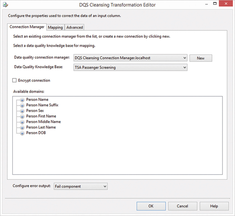
Figure 13.18 DQS cleansing transformation editor.
Create a new connection to the DQS server by using the new button. Once the connection is established, select the knowledge base configured in the previous section. The dialog will show domains found in the knowledge base.
Switch to the mapping tab to map the columns in the data flow to the domains in the knowledge base (Figure 13.19).
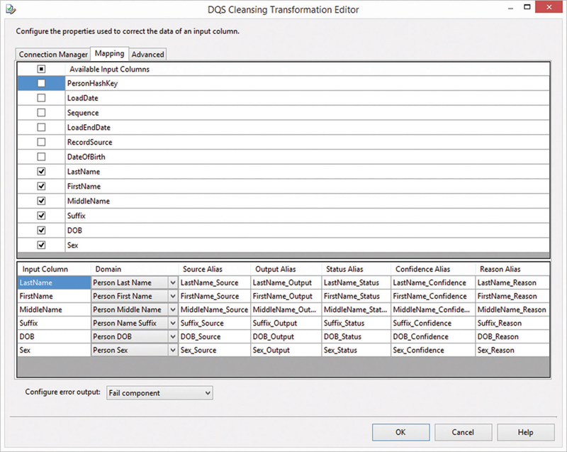
Figure 13.19 Mapping columns from the data flow to DQS domains.
Select the columns from the data flow that should be cleansed in the grid on the upper half of the dialog. In order to cleanse a column, a corresponding DQS domain is required. If there are other columns in the data flow without a corresponding domain in the knowledge base, they have to be added in DQS first (as in the previous section).
Map each selected input column to a DQS domain. Leave all other options (source alias, output alias, status alias, confidence alias and reason alias), as they are. These columns will provide useful information about the data cleansing operations to the business user. However, in order to actually include these informative columns in the output of the DQS cleansing transformation, switch to the advanced tab (Figure 13.20).

Figure 13.20 Advanced tab of DQS cleansing transformation editor.
Check all options to add all informative columns. The first option is used to standardize the output, which means that their standardized counterparts might replace domain values.
Close the dialog and add an OLE DB destination component to the data flow. Connect it to the DQS cleansing transformation. Open the editor of the OLE DB destination transformation to configure it (Figure 13.21).

Figure 13.21 OLE DB destination editor for target satellite in Business Vault.
Select the DataVault database and the target satellite in the Business Vault. Configure the column mapping between the data flow and the target table on the next page, shown in Figure 13.22.

Figure 13.22 Column mapping in the OLE DB destination editor.
The source columns from the DQS cleansing transformation are ignored because the same data is found in the raw satellite. The sequence from the source is added as a descriptive attribute to the target satellite (which is not a multi-active satellite) to retrieve the corresponding record from the source. The output columns are mapped to the cleansed attributes. All other attributes (status, confidence, and reason) are added and mapped to the target as well.
The final data flow is presented in Figure 13.23.

Figure 13.23 Data cleansing in SSIS.
Because the lookup is executed before the DQS cleansing takes place, the data is reduced to the records that are unknown to the target satellite and actually require data cleansing: all known records have been cleansed in the past.
Note that the ETL process to build a business satellite often doesn’t follow a prescribed template, as is the case when loading the Raw Data Vault as shown in Chapter 12, Loading the Data Vault. Instead, most business vault entities are loaded using individual processes, which is hard to automate.
To complete the process, it is required to end-date the target satellite. This approach, however, follows the standard end-dating process for satellites in the Raw Data Vault, outlined in Chapter 12.
To further improve the solution, the informative attributes from the DQS cleansing transformation could be loaded into a separate satellite instead of the same target. This would improve the usability and performance of the cleansed satellite.
The resulting satellite can be used as any other satellite in the Raw or Business Data Vault for loading the information marts.
13.9. Match and Consolidate Data
A typical task in data warehousing is to resolve identities that [36]:
• Represent the same entity: here, duplicate business keys or relationships from the same or different source systems mean the same business entity. The typical goal is to merge the business entities into one and consolidate the data from both records or remove duplicate data in favor of a master record.
• Represent the wrong entity: there are cases where the business user thinks that a record is not in the system because of a slight variation in the descriptive data, which leads to an unfound (yet existing) record [10].
• Represent the same household: in other cases, there are different business entities (identified as such) that belong together. For example, they live in the same household or work in the same organization. The goal is to aggregate the data to the higher order entity.
For all cases, there are entities in the Data Vault 2.0 model that support each of them. The resolution of duplicate identifiers for the same business entities can be solved with a same-as-link (SAL) that was introduced in Chapter 5. Errors in descriptive data can be fixed using computed satellites, similar to the approaches discussed in section 13.8. The last case can be solved with a hierarchical link.
This approach can be supported by a variety of techniques and tools, for example [3]:
• Data matching techniques: it is possible to identify potential duplicates using matching techniques, such as phonetic, match code, cross-reference, partial text match, pattern matching, and fuzzy logic algorithms [6].
• Data mining software: instead of relying on rules, data mining tools rely on artificial intelligence algorithms that find close matches.
• Data correction software: such software implements data cleansing and other algorithms to test for potential duplicate matches and merge the records.
The next section presents how to de-duplicate data using a fuzzy data matching algorithm included in SSIS.
13.9.1. SSIS Example
Fuzzy logic represents a fairly easy approach for data de-duplication and is supported by SSIS. The example in section 13.8.3 has demonstrated how to cleanse descriptive attributes in satellites. The satellite also contained duplicate data, describing similar persons. However, in order to cleanse the data, the hub has to be cleansed first.
The recommended approach for data de-duplication in Data Vault 2.0 is to take advantage of a same-as link, introduced in Chapter 5. By doing so, the raw data is left untouched and the concept provides the most flexibility.
The HubPerson is defined using the following DDL:

The business key of this hub is a composite key consisting of the attributes LastName, FirstName, MiddleName, and date of birth DOB, apparently because there was no passenger ID or person ID available in the source data. This is a weak way of identifying a person, with many possible false positive matches. The better approach is to use a business key for this identification purpose. However, the sample data doesn’t provide such a business key and, in reality, there are some cases where no business key for persons is available.
Create the following same-as link so it can be used as the data flow’s destination:

The same-as link is defined by two hash keys, which point to the same referenced hub, HubPerson. One of the hash keys references the master record; the other hash key references the duplicate record that should be replaced by the master in subsequent queries.
Create a new data flow and drag an OLE DB source component to it. Open the editor (Figure 13.24).

Figure 13.24 OLE DB source editor for HubPerson.
Because only data is used as descriptive input for the following fuzzy group process, no other descriptive data needs to be joined to the source. Therefore, the HubPerson in the Raw Data Vault is selected. If additional descriptive data should be considered in the de-duplication process, for example data from dependent satellites, the data should be joined in a source SQL command.
Make sure that all columns from the hub are included in the OLE DB source and close the dialog. Add a fuzzy grouping transformation to the canvas of the data flow and connect it to the source.
Because the fuzzy grouping algorithm is resource-intensive, it requires a database for storing temporary SQL Server tables. Create a new connection and specify the tempdb database (Figure 13.25).

Figure 13.25 Configuring tempdb for fuzzy grouping.
The advantage of the tempdb database is that every user has access to the database and created objects are dropped on disconnect [11]. In most cases, it is also configured for such applications. As an alternative, it is also possible to use another database for storing these temporary objects. You should consult your data warehouse administrator for more information.
Make sure the created tempdb connection manager is selected on the first page of the fuzzy grouping transformation editor (Figure 13.26).

Figure 13.26 Configuring the connection manager of the fuzzy grouping transformation.
Select the columns tab to set up the descriptive columns that should be used in the de-duplication process (Figure 13.27).

Figure 13.27 Setting up descriptive columns for de-duplication.
Select all descriptive columns and set the match type. For string columns, this should be fuzzy. In some cases, it makes sense to enforce the exactness of other attributes, as this is the case for the DOB column. This domain knowledge is usually provided by the business user.
Make sure that all other columns that are not used in the fuzzy grouping algorithm are activated for pass-through and switch to the advanced tab, shown in Figure 13.28.

Figure 13.28 Configuring advanced options in the fuzzy grouping transformation editor.
The similarity threshold influences which persons are considered as duplicates. The lower the threshold is, the more false-positive matches the algorithm will produce. On the other hand, keeping the value too high increases the number of false-negative matches:
• False-positive match: the fuzzy-grouping algorithm wrongly (false) thinks that two persons are the same (positive).
• False-negative match: the fuzzy-grouping algorithm wrongly (false) thinks that two persons are not the same (negative).
• True-positive match: the algorithms correctly (true) identified two persons as duplicates (positive).
• True-negative match: the algorithm correctly (true) classified both persons as different (negative).
While the default value of 0.80 is a good setting for most cases, the same-as link is capable of providing a better solution when setting this threshold to a lower value because it gives the user of the same-as link (the information mart or a power user) more choices. Therefore, set the threshold to a very low value of 0.05. This will produce a lot of false-negative matches, but section 13.10 will demonstrate that it doesn’t matter (not from a storage or usage perspective) but allows the user to use a user-defined threshold instead of relying on this constant value. It is only recommended to set the threshold to a higher value when dealing with large volumes of business keys in the source hub (regardless of any descriptive data).
The result that will be produced by the fuzzy grouping transformation is shown in Figure 13.29.

Figure 13.29 Output of fuzzy grouping transformation.
The transformation adds the columns defined in Figure 13.28 which are used as follows:
• _key_in: a surrogate key that identifies the original record. In the same-as link terminology, this is the duplicate key. The surrogate key was introduced by SSIS and is not coming from the source.
• _key_out: the surrogate key of the record that the record should be mapped to. This is the master key. If the record should not be mapped to another record, both surrogate keys are the same.
• _score: the similarity score of both records (the duplicate and the master record). If both are the same (and no mapping takes place), the similarity score is 1.0 (100% equal).
The problem with this output, which cannot be influenced much, is that the hash keys of the master and duplicate records are required for loading the target same-as link. The hash key that is in the data flow identifies the duplicate record. In order to add the hash key of the master, the easiest and probably the fastest way is to create a copy of the data and merge it back by joining over the surrogate keys.
Close the fuzzy grouping transformation editor, add a multicast transformation to the data flow and add two sort transformations, each fed from a path from the multicast transformation. The first sort transformation is configured to sort its own copy of the data flow by the surrogate key of the master record (Figure 13.30).

Figure 13.30 Configuration of the sort transformation of the master data flow.
Select the column _key_out for sorting and pass through all other columns. Close the dialog and open the configuration dialog for the second sort transformation, which sorts its copy of the data flow by the surrogate key of the duplicate record (Figure 13.31).

Figure 13.31 Configuration of the sort transformation of the duplicate data flow.
Select the surrogate key of the duplicate, which is _key_in. Enable pass-through for all other columns. Close the dialog and add a merge join transformation. Connect it to the outputs of both sort transformations and open the transformation editor (Figure 13.32).
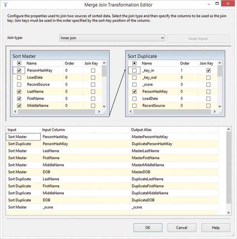
Figure 13.32 Merge join transformation editor for joining the master record to the duplicate record.
Connect _key_in from the duplicate data stream to _key_out from the master data stream with each other. This becomes the join condition. Select both hash keys and name them MasterPersonHashKey and DuplicatePersonHashKey. They will be written to the target link and reference the hub. Make sure to select all elements of the composite business key (LastName, FirstName, MiddleName, and DOB) from each stream. They are required in order to calculate the hash key for the same-as link. In addition, select the _score attribute from the duplicate data stream. It will be written to the target link as well.
Set the join type to inner join: there should be a matching master record in the second data flow.
Close the editor and connect the output of the merge join transformation to a new derived column transformation. It is used to calculate the hash key of the same-as link using the approach presented in Chapter 11, Data Extraction (see Figure 13.33).

Figure 13.33 Derived column transformation editor.
Add a load date to the stream and retrieve the load date of the current batch from the SSIS variable dLoadDate. Set the record source to an identifier for the soft rule. Calculate the input to be used for the link hash key (SALPersonHashKey) calculation using the following expression:

Make sure the name of the input column ends with “LinkBK” so that the hash function can catch up the business key automatically. Drag a script component to the canvas and connect it to the existing data flow. Its purpose is to calculate the hash key based on the input created in the last step. It follows the same approach as in Chapter 11.
Open the script transformation editor and switch to the input columns page (Figure 13.34).

Figure 13.34 Configuring the input columns in the script transformation editor.
Select the input column created in the previous step. Switch to the inputs and outputs tab and create a new output (Figure 13.35).

Figure 13.35 Configuring input and output columns in the script transformation editor.
Add a new output column to the existing output. Use the exact same name as the selected input column but ending with “HashKey” (refer to Chapter 11 for details). Use a string data type with a length of 32 characters and code page 1252 (or whatever code page is appropriate in your data warehouse environment). However, note that the hash key uses only characters from 0 to 9 and A to F. Switch to the script tab and add the script from Chapter 11.
Build the script and close both the script editor and the script transformation editor. Drag an OLE DB destination component to the data flow and connect it to the output of the script component. Open the editor to configure the target (Figure 13.36).

Figure 13.36 Configuring the same-as link target in the OLE DB destination editor.
Select the target link SALPerson in the Business Vault. Check keep nulls and table lock. Switch to the mappings tab to configure the mapping between the data flow and the target table (Figure 13.37).

Figure 13.37 Configuring column mapping for the same-as link in the OLE DB destination editor.
Make sure that each target column is sourced from the data flow. Close the dialog.
The final data flow is presented in Figure 13.38.

Figure 13.38 Data flow for de-duplication and loading same-as links.
There are two options to run this data flow in practice:
1. Incremental load: this approach requires updating entries when the scores or the mapping (from duplicate to master) change.
2. Truncate target before full load: in order to avoid the update, the target is truncated and reloaded with every run.
In most cases, the second option is much easier to use while still feasible from a performance standpoint. Only if the hub contains many records is incremental loading required.
13.10. Creating Dimensions from Same-As Links
The same-as link created in the previous section can be used as the foundation for a de-duplicated dimension:


Instead of sourcing the virtual view from the actual hub and its satellites, the same-as link is used as the source and the satellites, which still hang off the hub, are joined to the same-as link to provide descriptive data.
The previous statement uses the score value from the fuzzy grouping transformation to dynamically select the mappings between the (potential) duplicate and the master record in the parent hub. By providing this score value, a power user can adjust this constant value (in the above statement 0.5) to include more or fewer mappings into the dimension: the lower the constant is set, the more business keys are mapped to a master in the dimension. A higher value means that the confidence of the algorithm should be higher before mapping takes place.
..................Content has been hidden....................
You can't read the all page of ebook, please click here login for view all page.