10
Identification of Imagined Bengali Vowels from EEG Signals Using Activity Map and Convolutional Neural Network
Rajdeep Ghosh1*, Nidul Sinha2 and Souvik Phadikar2
1School of Computing Science and Engineering, VIT Bhopal University, Kotri Kalan, Madhya Pradesh, India
2Department of E.E., NIT Silchar, Silchar, Assam, India
Abstract
Classification of electroencephalogram (EEG) signals is challenging due to its non-stationary nature and poor spectral resolution w.r.t. time. This chapter presents a novel feature representation termed as activity map (AM) for the classification of imagined vowels from EEG. The proposed AM provides a visualization of the temporal and spectral information of the EEG data. The AM is created for each of the EEG recorded from 22 subjects imagining five Bengali vowels /আ/, /ই/, /উ/, /এ/, and /ও/ using 64 channels. The AM is generated by extracting the band power in delta, theta, alpha, beta, and gamma bands for each second of the EEG and subsequently stacking them to form a matrix. The matrix is then converted into a heat map of 100 × 200 pixels called AM. The AM thus obtained, is classified using a convolutional neural network (CNN), achieving an average accuracy of 68.9% in classifying the imagined vowels. The CNN demonstrates superior performance in comparison to other methods reported in the literature using various features such as common spatial pattern (CSP), discrete wavelet transform (DWT), etc. and with different classifiers such as kNN (k nearest neighbor), support vector machine (SVM), linear discriminant analysis (LDA), and multilayer perceptron neural network (MLPNN).
Keywords: Activity map, band power, brain-computer interface (BCI), convolutional neural network (CNN), electroencephalogram (EEG), imagined speech, silent speech (SS)
10.1 Introduction
The brain is a complex organ generating electrical and chemical responses. The electrical activity of the human brain was first measured by a German psychiatrist named Hans Berger in the year 1929 [16]. The works of Hans Berger have inspired many and the domain has developed since then, especially in the last decade. The potential for the application of the brain signals has generated quite a lot of interest in researchers and has paved the way for the development of a research area known as a brain-computer interface (BCI) which utilizes EEG signals for controlling devices. Besides, EEG signal processing is also being used extensively to analyze various neurological disorders like epilepsy, sleep study, etc.
The brain-computer interface (BCI) is an intermediate arrangement that allows the communication between the brain of an individual and an external output device. It first measures the brain activity of an individual relating to a particular task, after which it extracts features about that activity, and converts those features to generate a suitable output or control signals for an external device. BCIs are developed to improve or enhance certain functions in disabled individuals who have lost their muscular coordination due to diseases like paralysis, locked-in syndrome, injuries, etc. but have a functional brain. BCI serves as an alternative form of communication for such individuals. The measurement of the brain activity can again be carried out in multiple paradigms:
- Invasive: In the invasive method, a chip is implanted inside the head directly on the Gray matter of the brain, and as such produces a high-quality electrical signal capturing the electrical activity of the brain. But the major problem is that to implant a chip, neurological surgery is needed and has a very high risk of building-up of scar tissue in the operated part. Example: Local field potential (LFP) [17].
- Partially Invasive: In this method, the electrodes are placed to record the electrical activity inside the skull, but on the surface of the membrane that protects the brain. The signal quality is lower than the invasive method, but the risk of forming scar tissue is lower, but is not free from scar tissue formation. Example: Electrocorticography (ECoG) [17].
- Non-invasive: It is the most popular approach for recording brain signals. It is the safest way to record brain signals as the recording is done externally on the scalp. The electrodes or sensors are placed on the surface of the scalp. It produces a poor signal and low spatial resolution. Example EEG, functional magnetic resonance imaging (fMRI) [18].
10.1.1 Electroencephalography (EEG)
The neurons inside the brain communicate with each other with the help of electrical signals. These electrical signals can be measured with the help of electrodes placed at various locations on the scalp of an individual. EEG signals have been extensively used by neurologists to identify and treat different diseases such as epilepsy, Alzheimer’s disease, etc. associated with the brain. Besides, EEG can also be used for evaluating the sleep pattern of an individual, understand learning or attention disorders. Commonly Ag-AgCl electrodes are used as electrodes. The signal values obtained are in the range of 0.5–100 µV. EEG measures the voltage difference between the two electrodes [19].
EEG is one of the widely used devices in BCI for recording the excitation of the brain due to its non-invasive recording methodology, low cost, high temporal resolution, and ease of use. BCIs have been used in various applications like prosthetics, classifying emotions, etc. An important application of BCI has focused on the development of a communication interface for enabling paralyzed individuals to communicate with the external world [12, 15, 29]. The necessity for such an interface has led to the concept of recognition of speech from the human brain. The focus of this chapter is to describe an application of a well-known deep learning model known as the convolutional neural network (CNN) to classify imagined vowels from the EEG recordings of individuals.
10.1.2 Imagined Speech or Silent Speech
An interpretation of silent speech or imagined speech can be referred to as the words heard or conceived by an individual in his head without any vocalization to the environment. To understand imagined speech it is very essential to understand the stages of speech communication carried out by an individual. The first stage is the conceptualization and formulation of the speech which occurs in the brain. In this process, the communication intentions are converted into messages known as the surface structure following the grammatical rules of the language in which verbal communication is to be made. In the next step, the surface structure is converted to the phonetic plan, where a sequence of phonemes that form the speech is fed to the articulators. After which, electrical impulses are given to the articulators to start the articulation process. The final stage produces the acoustic speech signal as a result of the consequent effects from the previous phases. Hence, silent speech can be defined as speech originating inside the human brain which has not been vocalized by the individual [20]. Figure 10.1 represents the speech production process in an individual.

Figure 10.1 Speech production process by an individual.
The focus of the present study deals with identifying silent/imagined speech by measuring the electrical activity of the brain. The present chapter is concerned with the recognition of only five imagined Bengali vowels /আ/, /ই/, /উ/, /এ/, and /ও/ from the EEG recordings of an individual.
10.2 Literature Survey
The earliest efforts in this respect were made by Birbaumer et al. [1], who developed the thought translation device for locked-in patients using slow cortical potentials (SCP), which permits the users to select a particular letter in the English language for communication. Wester [2] classified mumbled, unspoken, silent, whispered, and normal speech, from EEG recordings by using linear discriminant analysis (LDA) as a classifier. He cited the importance of Wernicke’s area and Broca’s area in the brain for speech communication. DaSalla et al. [3] classified three imagined states: a state of no action, the imagination of the English vowel /a/, and the English vowel /u/ from three subjects by using a non-linear support vector machine (SVM). Brigham et al. [11] considered the recognition of two syllables /ba/ and /ku/ from the EEG recorded from seven subjects. In their work, the EEG data were pre-processed to reduce the effects of artifacts and noise using independent component analysis (ICA). After the removal of artifacts from the EEG, autoregressive (AR) coefficients were evaluated for the classification of imagined syllables using a kNN classifier. They obtained an average classification accuracy of 61% in classifying the syllables, which suggests that it was possible to identify imagined speech syllables from the EEG.
Calliess [21] further extended the works carried out by Wester [2] and placed electrodes primarily in the orofacial motor cortex with a different cap arrangement to capture the EEG data more efficiently. In this work, it was further established that the successful recognition rate in [2] was due to the temporal correlation among the EEG data created during the collection of the data. It was further reported that the repeated imagination of a word created a high recognition rate. However, the accuracy dropped if the EEG data for the words were recorded in random order.
Mesgarani et al. [22] measured the electrical activity from the primary auditory cortex in response to sentences from the Texas Instruments (TI) and Massachusetts Institute of Technology (TIMIT) database. They examined the effect of various phonemes on the different subsets of auditory neurons. Their study reflected that the neurons with different spectro-temporal tuning responded differently in response to specific auditory stimuli, which could be represented explicitly in a multidimensional articulatory feature representation, which is independent of the speaker and the context. Galgano and Froud [23] established the existence of voice-related cortical potentials (VRCP) in their study. They used a 43 channel EEG instrument to record the neuronal activity of the subjects who were instructed to hum in response to a stimulus and found a slow, negative cortical potential before 250 msec from the start of phonation by the subjects.
Efforts have also been made by D’Zmura et al. [24] for recognizing imagined syllables from the EEG recordings. They considered two syllables /ba/ and /ku/ for recognition. 20 EEG trials were recorded from four subjects under six experimental conditions where the syllables were presented in a randomized order of the subjects. Analysis of the EEG was carried out w.r.t. the three bands theta, alpha, and beta bands showing the presence of information. Envelopes were created using Hilbert transformation to compute matched filters corresponding to the particular imagined syllable to yield the degree of similarity in the respective EEG bands. The classification accuracy achieved was around 60%. However, the removal of electrodes containing the artifacts resulted in the loss of neural information for the recognition of the syllables in their work.
Santana [25] in his work classified two English vowels /a/ and /u/ from the EEG recordings of three subjects. Spatial filters were evaluated using CSP and then classified. The performance of classification was analyzed for 10 classifiers. He concluded that simple classifiers like Gaussian naive Bayes classifier outperformed the SVM classifier. He further added that different classifiers exploit different mental mechanisms and subjects could be grouped based on the underlying mental mechanisms. Matsumoto [26] investigated the classification of two imagined vowels in Japanese similar to /a/ and /u/ obtained from 4 subjects who were imagining the vocalization of those vowels using 63 EEG channels. An adaptive collection (AC) was used for classification. The obtained accuracy of classification was in the range of 73–92%. Kamalakkannan et al. [27] tried to classify imagined English vowels /a/, /e/, /i/, /o/, and /u/ in their work. EEG data were recorded from 13 subjects using 20 electrodes. They extracted the following features from the EEG recordings: standard deviation, mean, variance, and average power, which were classified using a bipolar neural network. Maximum accuracy of 44% was obtained in their work. Their results showed that some distinctive information was present in the EEG relating to imagined vowels. They also found that the increase in relaxation time increased the classification accuracy. They also suggested that the classification could be extended to major 36 alphanumeric characters.
Salama et al. [28] classified two imagined words, namely, ‘yes’ and ‘no’ from the electroencephalographic signals recorded using only a single electrode EEG device. The single electrode setup was adopted in their work due to the following advantages: ease of setup, adjustment, and light weight. Data were recorded from 7 subjects who were imagining the words in response to specific questions. Wavelet packet decomposition was applied to extract features from the EEG and was classified using 4 classifiers: support vector machine (SVM), self-organizing map (SOM), discriminant analysis (DA), feed-forward network (FFN), and ensemble network (EN). The average online classification rate was 57% and the offline recognition rate was 59%.
Nguyen et al. [10] used a covariance matrix descriptor from the Riemannian manifold as features to classify EEG recordings relating to the imagined pronunciation of long words, short words, and vowels collected from a total of 15 subjects, which were subsequently classified using relevance vector machines (RVM) classifier. They achieved an accuracy of 70% in classifying the words from the EEG recordings and concluded that certain aspects such as word complexity, meaning, and sound may affect the classification of the imagined speech from the EEG signals.
Wang et al. [30] classified between motor imagery and speech imagery signals collected from 10 subjects and achieved an accuracy of 74.3% for classification of mental tasks in speech imagery, 71.4% in imagining left-hand movement, and 69.8% in imagining right-hand movement. Time-frequency characteristics were estimated from the EEG signals by using event-related spectral perturbation (ERSP) diagrams which provide a good time-frequency visualization. EEG signals recorded for different imageries have different energy changes which can be extracted using CSP. Moreover, it was observed that the synchronization in the cerebral cortex was different for speech imagery and motor imagery. Recently, Bakshali et al. [4] classified EEG data relating to the imagination of words and syllables from the “Kara One” database by using the Riemannian distance evaluated from the correntropy spectral density (CSD) matrices and achieved a significant classification accuracy of 90.25%. The CSD matrix does not contain any frequency information about the channels, but it does contains some similar information regarding the channels. However, an appropriate pre-processing method is essential for achieving a good classification accuracy.
Sereshkeh et al. [13] recorded the EEG from 12 participants who were performing the mental imagination of two words “yes” and “no”. The EEG was recorded in two sessions for multiple iterations. The individual duration of the EEG recording was 10 seconds. Discrete wavelet transform (DWT) based features were evaluated from the EEG data which were classified using a multilayer perceptron neural network (MLPNN). Average accuracy of 75.7% was achieved in their case. Chi et al. [14] classified five types of imagined phonemes that differ in their vocal articulation (jaw, tongue, nasal, lips, and fricative) during speech production. Spectrogram data were directly used for classifying the EEG data. LDA and Naive Bayes (NB) classification methods were used to classify the EEG signals. The classification accuracy varied from 66.4% to 76% on the data collected in multiple sessions. Their results showed that the signals generated during the imagination of phonemes could be differentiated from the EEG generated during periods when there was no imagination by the subjects.
EEG signals are non-stationary and hence present a challenge in their classification. The primary issue remains in identifying suitable features to discriminate between the EEG signals. A variety of methods have been used in the literature to classify silent speech phonemes, syllables from EEG. The methods available in the literature focus on extracting spatial, temporal, and spectral features from the EEG signals to classify imagined speech. Temporal features of the EEG like energy, power, etc. have been used for classifying the imagined speech. Common spatial pattern (CSP) and their variants have been widely used in the literature to classify imagined speech. Besides, ICA has also been used in the literature to process the EEG related to the imagined speech. The usefulness of ICA lies in its ability to separate independent components from the EEG. Various methodologies based on Fourier transform (FT), wavelet transform (WT) have also been used to extract spectral features from the EEG relating to imagined speech. Besides, statistical features like mean, variance, standard deviation, etc. have also been used for the classification of imagined speech. However, selecting features reflecting only temporal or spectral information does not allow an efficient recognition of imagined speech from EEG. It is essential to consider features that reflect different properties of the EEG signal. Hence, the proposed work presents a novel activity map (AM), to represent the changes in various frequency bands w.r.t time.
Deep learning-based methodologies like CNN, autoencoder, etc. have been used to solve a wide variety of problems in recent times. Deep learning methodologies have also been applied for processing EEG signals [5]. The benefit of using deep learning is its ability to learn complex representations from the data. The novel AM generated in the present work is classified using CNN. CNN’s have proved their efficiency to classify images and hence have been selected for classification of the AM relating to the respective EEG of the imagined speech. Although various methodologies are available for classifying silent speech from EEG, yet they fail to classify them effectively. Hence, a novel methodology has been developed to classify the imagined speech from EEG.
10.3 Theoretical Background
The work presented in this chapter is focused on the identification of the imagined Bengali vowels from EEG and utilizes the concept of the convolutional neural network to classify the activity maps (AMs) representing the different imagined Bengali vowels. The description of the various concepts is described in this section.
10.3.1 Convolutional Neural Network
Convolutional neural networks originate from the works of Fukushima in 1980 [7] but have seen rapid development recently and have been applied to a variety of applications related to image processing, video processing, drug discovery, etc. A CNN comprises of an input layer, multiple hidden layers, and an output layer. The hidden layers are comprised of numerous convolution layers, pooling layers, flattening layers, followed by a fully connected layer. A typical CNN includes the following layers: convolutional layer, activation layer, pooling layer, flattening layer, a fully connected/ dense layer, and a classification layer. The convolutional layer convolves the input image with a set of R filters and adds the respective bias value, which is then forwarded to a nonlinear activation function to generate feature maps:
 (10.1)
Where θ(i) represents an m×n image with c channels, Xr represents the r-th convolution filter or a kernel with dimension s×s, * denotes the convolution operation, and br represents the bias term for the r-th filter, R represents the total number of filters, and g() represents the activation function [8]. Different activation functions can be applied in the activation layer. Rectified linear unit (ReLU) function is one of the most commonly used activation functions in CNN and can be described as:
 (10.2)
The pooling layer downsamples the feature matrix to lower dimensions. The pooling operation reduces the number of computations and also removes the redundant information while training the CNN. Max-pooling and average-pooling are the two of the most used techniques. The former method selects the maximum pixel value as the representation of a small pooling region, while the latter uses the average value of this region as the representation. The pooling layer is succeeded by a flattening layer, which converts the two-dimensional vector to a one-dimensional vector. The flattening layer is succeeded by a fully connected/dense layer which in turn is connected to the classification layer.
The classification layer has nodes equal to the number of classes in the problem for which the CNN is trained. The softmax activation function is generally used for classification as it provides the output in terms of probability ranges. The layer provides output values between 0 and 1 and the sum of probabilities of the data belonging to a particular class is equal to one. Mathematically the output probability of a node can be expressed as:
 (10.3)
z denotes the output value of the node in the softmax layer and N denotes the number of classes.

Figure 10.2 Transformation of the image across different layers of CNN.
Figure 10.2 represents the transformation of an image in a CNN. Initially, RGB images can be given as input to the CNN, which is gradually transformed into a 2-dimensional matrix after convolution and pooling. The 2-dimensional matrix is then transformed to a 1-dimensional vector after which an output class label is finally generated. CNN’s can be organized in various dimensions and can be utilized for different applications.
10.3.2 Activity Map
The present work describes the creation of a novel activity map (AM), which represents the tempo-spectral information of all the EEG channels which is subsequently converted into an image. EEG signals are categorized into five primary frequency bands delta (f<4 Hz), theta (4≤f<7 Hz), alpha (8≤f<13 Hz), beta (13≤f<30 Hz), and gamma (30 Hz<f) bands based on the nature of the different states in the brain like relaxed, active, etc. Hence, it is essential to capture the activity of a particular band, and band power serves as a useful metric for obtaining the information in a specific frequency band. Band power specifies the average power in a respective frequency band and represents the activity in an individual frequency band. Band power reflects the average power in a particular frequency band. The average power of the signal x[t] within a window of size w can be represented as:
 (10.4)
This means the power is averaged over window w over which the frequency is estimated. p[n] represents the power spectral density of a particular frequency. The procedure to generate the AM is as follows: Let us consider an EEG signal of 5 seconds with 64 channels. The EEG signal for all the channels is split into segments of one second each. From the one-second segment, the band power is evaluated in the respective frequency bands: delta, theta, alpha, beta, and gamma bands. The band power thus obtained is placed sequentially one after the other giving a total of 25 values (5 sec. × 5 Band power values for each band) for an individual channel. The values, thus obtained are stacked for all the 64 channels yielding a matrix of size 64 × 25. The matrix, thus obtained is converted into a heat map of 100 × 200 pixels. Figure 10.3 represents an AM generated in the proposed work. The AM represents the activity in a particular frequency band with respect to the time.
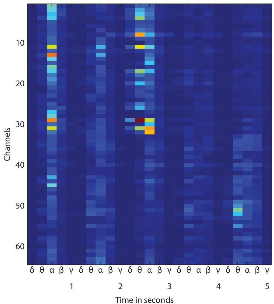
Figure 10.3 Activity map for an EEG trial.
10.4 Methodology
The proposed work is focused on the classification of the imagined Bengali vowels from EEG, and in this regard, a novel feature extraction methodology has been developed known as AM, which is subsequently converted into an image and classified with the help of a CNN.
The methodology of the proposed work is described in Figure 10.4. The different phases of the overall methodology are follows:
- Data collection: Initially, the picture as well as the sound of the vowels are presented to the subject, after which the subject is instructed to imagine the sound of the vowel for 5 seconds in his mind. During the imagination of the vowel by the subject, the EEG of the individual is recorded. The EEG recording from an individual is conducted for five trials for each of the 5 Bengali vowels /আ/, /ই/, /উ/, /এ/, and /ও/ and the procedure has been described in Section 10.4.1.
- Data pre-processing: The EEG data collected from different individuals are segmented to extract the part of the EEG data containing the imagination of the vowels. The EEG data is very sensitive and is often corrupted with artifacts. The EEG data is then processed to remove artifacts and noise. The removal of artifacts and noise from EEG is a complex procedure and requires the usage of different methods and has elaborated in Section 10.4.2. After the removal of artifacts, the EEG signal corresponding to the respective Bengali vowel is labeled.
- Generation of activity map: The objective of the proposed work is concerned with the classification of the imagined Bengali vowels from the EEG of an individual. For the purpose of classification, activity map is generated from the processed EEG obtained after the pre-processing step. The activity map is generated according to the procedure described in Section 10.3.2. The activity map corresponding to the respective EEG is saved as an image file in .jpeg format and is then used for the purpose of classification.

Figure 10.4 The methodology of the proposed work.
- Classification of the activity map using CNN: The activity map generated in the previous step is saved as an image file. CNN has proved to be efficient for the purpose of image classification and is therefore adopted in the present task for the purpose of classification. The architecture of the CNN has been described in Section 10.4.4. The AM’s corresponding to the different classes are then randomly split in 70:30 ratio for training and testing respectively and are fed to the CNN for the purpose of classification.
10.4.1 Data Collection
Data were collected at the National Institute of Technology, Silchar. A total of 22 subjects (16 Males, 6 Females) aged between 20–34 years took part in the experiment. The experiment was conducted after obtaining adequate permission from the authority and written consent from the subjects. The vowels considered for imagination were /আ/, /ই/, /উ/, /এ/, and /ও/. The reason for selecting the respective vowels is that the vowels resemble the pronunciation of the English language vowels /a/, /i/, /u/, /e/, /o/ respectively according to the International Phonetic Alphabet (IPA) which is a system of phonetic notation. 64 channel EEG was recorded using the standard 10–20 recording setup. The EEG data were sampled at 512Hz, and 5 trials were recorded for each vowel in the case of each individual reaching a total of 550 trials (22 Subjects × 5 Trials × 5 vowels). Figure 10.5 depicts the trial recording protocol followed in the present work for recording the EEG. Initially, the EEG recording cap is attached to the scalp of the subject after which, the subjects were asked to relax for 2 seconds, after which an audio-visual stimulus of the vowel to be imagined was presented to the subject for a duration of 4 seconds, the next phase was the fixation phase of 4 seconds where the subjects were instructed to focus on a fixed point at the center of the display screen, where the audio-visual stimulus was presented previously. After fixation, the vowel to be imagined was then displayed on the screen for 5 seconds, during which the subject was asked to imagine the vowel.
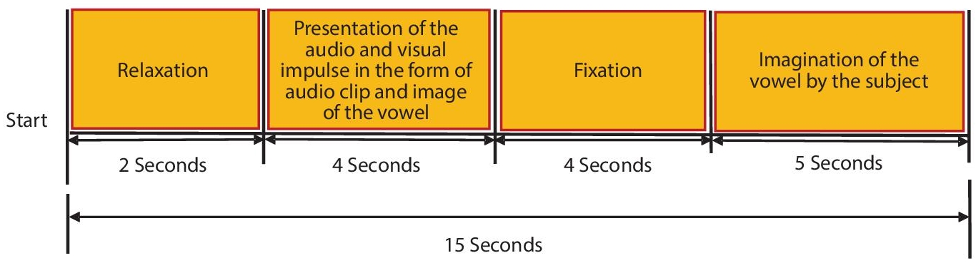
Figure 10.5 Trial recording protocol.
10.4.2 Pre-Processing
The pre-processing stage is primarily concerned with the removal of artifacts and noise from the EEG followed by the extraction of the segment of the EEG signal containing the imagination of vowels. Initially, it is observed that the data is corrupted by a 50 Hz power-line noise. Hence, a notch filter is applied to remove the same. After which the signals are filtered in the range of 0–60 Hz. After filtering the data, artifacts were removed from the EEG data using a hybrid method combining SVM and autoencoder which has been described in one of our previous works [6].
Figure 10.6 represents an EEG recording before the artifact removal. The artifacts are removed using a combination of autoencoder and SVM classifier. The SVM classifier has been used for the detection of artifacts and the autoencoder has been used for correcting the identified artifacts. The artifact removal methodology has been described in [6]. The artifact removal methodology adopted in our previous work follows a windowed strategy, where a window size of 0.45 seconds is slid forward to traverse the entire signal. A pre-trained SVM classifier classifies the selected EEG window as corrupted or uncorrupted. If the window is identified as corrupted, it is forwarded to the autoencoder for correction. The autoencoder is trained to generate clean EEG segments from corrupted segments. On the other hand, if the window is not corrupted, the algorithm moves to the next window. Figure 10.7 represents the 64 channel EEG after the application of the artifact removal procedure. The final phase involves trimming the signal to keep the final 5 seconds of the data containing the imagination of the vowels by the subjects.

Figure 10.6 EEG data contaminated with eye blink and muscle artifacts.

Figure 10.7 Channel EEG data corrected with SVM and autoencoder [6].
10.4.3 Feature Extraction
The proposed work focuses on the classification of imagined Bengali vowels from the EEG recordings of the subjects. The activity map is generated according to the procedure described in Section 10.3.2. The activity map provides a good time-frequency visualization of the EEG data. Moreover, it provides a visualization of the EEG activity only in the specific range of interest i.e., the delta, theta, alpha, beta, and gamma bands.

Figure 10.8 (a) Average activity map for the vowel /আ/. (b) Average activity map for the vowel /ই/. (c) Average activity map for the vowel /উ/. (d) Average activity map for the vowel/এ/. (e) Average activity map for the phoneme /ও/.

Figure 10.9 Average band power of the frequency bands.
Besides, the AM also creates a repetitive pattern which would be useful while classifying using CNN. The AM is generated from the trimmed EEG of all the 550 EEG trials. Figures 10.8(a), (b), (c), (d), and (e) represent the average activity maps of all 22 subjects for the imagined Bengali vowels /আ/, /ই/, /উ/, /এ/, and /ও/ respectively. From the average activity maps, it is clear that the activity maps provide a good differentiation among the EEG data representing the imagined Bengali vowels. Figure 10.9 depicts an average band power for the respective frequency bands obtained from all EEG segments. It can be inferred that the alpha band shows the maximum activity in comparison to other bands, thus confirming the wakeful-imaginative state of the subjects during recording.
10.4.4 Classification
The AM obtained during the process of feature extraction is classified with the help of a CNN. The architecture of the CNN used in the proposed work has been described in Table 10.1. The strategy adopted in designing the CNN is to subsequently reduce the dimension of the feature map. Table 10.1 describes the various layers used in the proposed work for the classification of the imagined vowel. The convolution layer uses the convolution operation to convert the image with a set of 192 filters to generate feature maps. The rectified linear unit (ReLU) serves as the activation function for the convolution layer. The advantage of ReLU lies in the fact that it is easier to compute and does not activate all the nodes at a time. The pooling layer combines the neighboring pixels into a single pixel, decreasing the dimension of the feature map generated. The normalization layer normalizes the gradients and activations in the network, thereby easing the training process of the network. The softmax layer normalizes the output of the fully connected layer, and the classification layer uses the probabilities of the softmax layer to assign labels to the individual input. The properties of the various layers are mentioned in Table 10.1. ReLU layer, followed by a max-pooling layer with the filter size of the preceding convolutional layer, was used after each convolutional layer. After four convolutional + ReLU + Max-pooling layers, a flattening layer was added, after which a fully connected layer with 5 nodes was added, followed by a softmax layer with 5 units and the final classification layer. In the proposed CNN, a stride of 2 has been selected in the convolutional and max-pooling layers.
Table 10.1 Description of the various layers of CNN used in the proposed work.
| Layer number | Quantity | Property of the layer |
| 1 | Image input layer | Size of image: 100×200×3 |
| 2 | Convolutional layer | No. of filters: 192; Size of the filter: 20×20; Stride: 2 |
| 3 | ReLU layer | -------------- |
| 4 | Max pooling layer | Size of filter: 20×20; Stride: 2 |
| 5 | Convolutional layer | No. of filters: 128; Size of the filter: 10×10; Stride: 2 |
| 6 | ReLU layer | -------------- |
| 7 | Max pooling layer | Size of the filter: 10×10; Stride: 2 |
| 8 | Convolutional layer | No. of filters: 64; Size of the filter: 3×3; Stride: 2 |
| 9 10 | ReLU layer Max pooling layer | --------------Size of the filter: 3×3; Stride: 2 |
| 11 | Convolutional layer | No. of filters: 32; Size of the filter: 1×1; Stride: 2 |
| 12 | ReLU layer | -------------- |
| 13 | Max pooling layer | Size of the filter: 3×3; Stride: 2 |
| 14 | Flattening layer | ---------------------- |
| 15 | Fully Connected Layer | Size: 5 |
| 16 | Softmax Layer | Size: 5 |
| 17 | Classification Layer | Evaluates one out of the 5 class label depending on the probability obtained from the softmax layer |
10.5 Results
MATLAB R2019b has been used to develop the proposed methodology and run on an Intel i7 processor with 8GB RAM. The data was split randomly in the 70:30 ratio for training and testing, respectively. The AM was formed from the EEG segments representing the imagination of the vowels /আ/, /ই/, /উ/, /এ/, and /ও/, which was given to the proposed CNN for classification. The average classification accuracy of the CNN in identifying the individual vowels is represented in Table 10.2. It is observed from Table 10.2 that the CNN achieves an accuracy of 68.9% in classifying the imagined vowels. The precision obtained in classifying the imagined vowels /আ/, /ই/, /উ/, /এ/, and /ও/ are 73.9%, 66.6%, 69.5%, 68.1% and 59.1% respectively. Besides, the CNN is also compared with different methodologies described in the literature for the identification of silent speech from EEG. It has been observed that the different methodologies described in the literature have used different combination of features and classifiers such as: autoregressive (AR) coefficients as feature and kNN as classifier [11], CSP as a feature, and SVM as classifier [9], spectrogram as a feature and LDA as classifier [14], DWT coefficients as features and MLPNN as classifier [13], and Riemannian distance (RD) evaluated from the correntropy spectral density (CSD) matrices as features and kNN as classifier [4]. F1 scores have been adopted for comparing the proposed CNN with the different methodologies. F1 scores are an efficient measure to distinguish between two classifiers when multiple classes are present. F1 scores balances between precision and recall and is therefore adopted for comparison with other classifiers. F1 scores can be computed as:
Table 10.2 Performance metrics for the individual imagined Bengali phoneme.
| Imagined vowel | Precision % | Recall % | F1 score | Overall accuracy % |
| /আ/ | 73.9% | 77.2% | 75.5% | 68.9% |
| /ই/ | 66.6% | 60.8% | 63.6% | |
| /উ/ | 69.5% | 66.6% | 68.1% | |
| /এ/ | 68.1% | 65.2% | 66.7% | |
| /ও/ | 59.1% | 68.4% | 63.4% | |
| Average: | 67.5% | 67.7% | 67.5% |
 (10.5)
Figure 10.10 presents the F1 score obtained using the proposed AM and CNN in comparison to the methodologies described in [4, 9, 11, 13, 14]. The F1 scores obtained by CNN are 75.5%, 63.6%, 68.1%, 66.7%, and 63.4% respectively for the imagined vowels /আ/, /ই/, /উ/, /এ/, and /ও/, which is higher in comparison to the methodologies described in [4, 9, 11, 13, 14].
However, the F1 score obtained for the Bengali vowel /ই/ is lower in comparison to the methods described in [4, 9]. The F1 score obtained using the Riemannian distance as features and kNN as a classifier [4] are: 69.54%, 65.12%, 63.2%, 64.32%, and 62.3% for the vowels /আ/, /ই/, /উ/, /এ/, and /ও/ respectively. The F1 score obtained using the methodology described by Matsumoto et al. [9], which used CSP as a feature and SVM as classifier were: 62.48%, 65.23%, 67.2%, 61.5%, and 60.7% for the vowels /আ/, /ই/, /উ/, /এ/, and /ও/ respectively. Similarly, the F1 score obtained using the methodology described by Brigham et al. [11], which used autoregressive coefficients as feature and kNN as classifier were: 55.23%, 59.3%, 58.4%, 54.2%, and 51.2% for the vowels /আ/, /ই/, /উ/, /এ/, and /ও/, respectively. The F1 score obtained using the methodology described by Sereshkeh et al. [13], which used DWT coefficients as a feature and MLPNN as classifier were: 53.2%, 54.3%, 55.4%, 54.2%, and 51.2% for the vowels /আ/, /ই/, /উ/, /এ/, and /ও/ respectively. The F1 score obtained using the methodology described by Chi et al. [14], which used spectrogram as a feature and LDA as classifier were: 44.3%, 53.2%, 49.5%, 51.6%, and 50.9% for the vowels /আ/, /ই/, /উ/, /এ/, and /ও/ respectively.
![Schematic illustration of F1 score comparison of the CNN w.r.t. the methodologies described in [4].](https://imgdetail.ebookreading.net/2023/10/9781119857204/9781119857204__9781119857204__files__images__c10_image_21_1.jpg)
Figure 10.10 F1 score comparison of the CNN w.r.t. the methodologies described in [4] which use Riemannian distance as features and kNN as the classifier, CSP as a feature and SVM as classifier [9], autoregressive coefficients as feature and kNN as classifier [11], DWT coefficients as features and MLPNN as classifier [13], and spectrogram as a feature and LDA as classifier [14].
From Figure 10.10, it is clear that CNN outperforms the other methodologies described in [4, 9, 11, 13, 14] in the majority of the cases. The methods described in [4, 9, 11, 13, 14] use various feature extraction methodologies such as AR coefficients, CSP, DWT coefficients, and RD along with kNN, SVM, LDA, and MLPNN classifiers. F1 scores obtained for the various methods establishes the suitability of the proposed AM and the CNN for the classification of the individual vowels.
10.6 Conclusion
The proposed work describes a novel feature extraction mechanism known as the activity map (AM) which captures the tempo-spectral information for the classification of the EEG related to the imagination of Bengali vowels আ/, /ই/, /উ/, /এ/, and /ও/. It is difficult to visualize the variation in the EEG data and hence, the AM provides a useful visualization of the spectral changes in EEG data w.r.t. time. The activity map is transformed into an image, which is subsequently classified with a CNN network with 4 convolutional layers. The average accuracy obtained in the overall classification is 68.9%. Moreover, it has also been observed that CNN outperforms other methods using various feature extraction methodologies such as AR coefficients, CSP, DWT coefficients, and RD along with kNN, SVM, LDA, and MLPNN classifiers. Hence, it can be concluded that the proposed AM in conjunction with CNN can classify the EEG data relating to the imagination of vowels effectively.
Acknowledgment
This work was supported by the Ministry of Communications & Information Technology No. 13(13)/2014-CC&BT, Government of India, for the project: ‘Analysis of Brainwaves and development of intelligent model for silent speech recognition’.
References
- 1. Birbaumer, N. et al., The thought translation device (TTD) for completely paralyzed patients. IEEE Trans. Rehabil. Eng., 8, 2, 190–193, June 2000.
- 2. Wester, M., Unspoken speech recognition based on electroencephalography, Thesis, Carnegie Mellon University, Pittsburgh, PA, USA, 2006.
- 3. DaSalla, C., Kambara, H., Sato, M., Koike, Y., Single-trial classification of vowel speech imagery using common spatial patterns. Neural Netw., 22, 1334– 1339, 2009.
- 4. Bakhshali, M.A., Khademi, M., Ebrahimi Moghadam, A., Moghimi, S., EEG signal classification of imagined speech based on Riemannian distance of correntropy spectral density. Biomed. Signal Process. Control, 59, 1–11, May 2020.
- 5. Samanta, K., Chatterjee, S., Bose, R., Cross-subject motor imagery tasks EEG signal classification employing multiplex weighted visibility graph and deep feature extraction. IEEE Sens. Lett., 4, 1, 1–4, Jan. 2020.
- 6. Ghosh, R., Sinha, N., Biswas, S.K., Automated eye blink artefact removal from EEG using support vector machine and autoencoder. IET Signal Process., 13, 2, 141–148, 2019.
- 7. Fukushima, K., Neocognitron: A self-organizing neural network model for a mechanism of pattern recognition unaffected by shift in position. Biol. Cybern., 36, 193–202, 1980.
- 8. Phang, C., Noman, F., Hussain, H., Ting, C., Ombao, H., A multi-domain connectome convolutional neural network for identifying Schizophrenia from EEG connectivity patterns. IEEE J. Biomed. Health Inform., 24, 5, 1333– 1343, May 2020.
- 9. Matsumoto, M. and Hori, J., Classification of silent speech using support vector machine and relevance vector machine. Appl. Soft Comput., 20, 95–102, 2014.
- 10. Nguyen, C.H., Karavas, G.K., Artemiadis, P., Inferring imagined speech using EEG signals: A new approach using Riemannian manifold features. J. Neural Eng., 15, 1–16, 2018.
- 11. Brigham, K. and Kumar, B.V.K.V., Imagined speech classification with EEG signals for silent communication: A preliminary investigation into synthetic telepathy. 2010 4th International Conference on Bioinformatics and Biomedical Engineering, Chengdu, pp. 1–4, 2010.
- 12. Yamaguchi, H. et al., Decoding silent speech in Japanese from single trial EEGS: Preliminary results. J. Comput. Sci. Syst. Biol., 8, 5, 285–291, 2015.
- 13. Sereshkeh, A.R., Trott, R., Bricout, A., Chau, T., EEG classification of covert speech using regularized neural networks. IEEE/ACM transactions on audio, speech, and language processing, vol. 25, pp. 2292–2230, 2017.
- 14. Chi, X. et al., EEG-based discrimination of Imagined speech phonemes. Int. J. Bioelectromagn., 13, 4, 201–206, 2011.
- 15. Ghane, P., Silent speech recognition in EEG-based brain computer interface, Master’s Thesis, Purdue University Graduate School, Indianapolis, Indiana, USA, 2015.
- 16. Wolpaw, J.R. et al., Brain-computer interfaces for communication and control. Clin. Neurophysiol., 113, 797–791, 2002.
- 17. Hassanien, A.E. and Azar, A.T., Brain-Computer Interfaces Current trends and applications, Springer, Switzerland, 2015.
- 18. Richards, T.L. and Berninger, V.W., Abnormal fMRI connectivity in children with dyslexia during a phoneme task: Before but not after treatment. J. Neurolinguistics, 21, 4, 294–304, 2008.
- 19. Mihajlovi, V., Garcia-Molina, G., Peuscher, J., Dry and water-based EEG electrodes in SSVEP-based BCI applications, in: Biomedical engineering systems and technologies, vol. 357, pp. 23–40, Springer, Berlin, 2013.
- 20. Freitas, J. et al., An Introduction to silent speech interfaces, Springer, Switzerland, 2017.
- 21. Calliess, J., Further investigations on unspoken speech. - findings in an attempt of developing EEG-based word recognition, Bachelor work, Interactive Systems Laboratories Carnegie Mellon University, Pittsburgh, PA, USA and Institut fuer Theoretische Informatik Universitaet Karlsruhe (TH), Karlsruhe, Germany, 2006.
- 22. Mesgarani, N., David, D., Sharma, S., Representation of phonemes in primary auditory cortex: How the brain analyzes speech. IEEE International Conference on Acoustics, Speech and Signal Processing, Honolulu, HI, USA, pp. 765–768, 2007.
- 23. Galgano, J. and Froud, K., Evidence of the voice related cortical potential: An electroencephalographic study. NeuroImage, 41, 1313–1323, 2008.
- 24. D’Zmura, M. et al., Toward EEG sensing of imagined speech, Human-Computer Interaction. Part I, HCII 2009, vol. LNCS 5610, pp. 40–48, 2009.
- 25. Santana, R., A detailed investigation of classification methods for vowel speech imagery recognition, in: Technical report, department of computer science and artificial intelligence, University of the Basque Country, San Sebastian, Spain, 2013.
- 26. Matsumoto, M., Silent speech decoder using adaptive collection. Proceedings of the companion publication of the 19th international conference on Intelligent User Interfaces, Haifa, Israel, pp. 73–76, 2014.
- 27. Kamalakkannan, R. et al., Imagined speech classification using EEG. Adv. Biomed. Sci. Eng., 1, 2, 20–32, 2014.
- 28. Salama, M. et al., Recognition of unspoken words using electrode electroencephalographic signals. 6th International Conference on Advanced Cognitive Technologies and Applications, COGNITIVE 2014, pp. 51–55, 2014.
- 29. Ghosh, R., Kumar, V., Sinha, N., Biswas, S.K., Motor imagery task classification using intelligent algorithm with prominent trial selection. J. Intell. Fuzzy Syst., 35, 2, 1501–1510, 2018.
- 30. Wang, L. et al., Analysis and classification of hybrid BCI based on motor imagery and speech imagery, Measurements, 147(20190), 106842, 1–12, 2019.
Note
- *Corresponding author: [email protected]