
Chapter 6. Deep Learning and AI
We begin this chapter with an overview of the machine intelligence landscape from Shivon Zilis and James Cham. They document the emergence of a clear machine intelligence stack, weigh in on the “great chatbot explosion of 2016,” and argue that implementing machine learning requires companies to make deep organizational and process changes. Then, Aaron Schumacher introduces TensorFlow, the open source software library for machine learning developed by the Google Brain Team, and explains how to build and train TensorFlow graphs. Finally, Song Han explains how deep compression greatly reduces the computation and storage required by neural networks, and also introduces a novel training method—dense-sparse-dense (DSD)—that aims to improve prediction accuracy.
The Current State of Machine Intelligence 3.0
You can read this post on oreilly.com here.
Almost a year ago, we published our now-annual landscape of machine intelligence companies, and goodness have we seen a lot of activity since then. This year’s landscape (see Figure 6-1) has a third more companies than our first one did two years ago, and it feels even more futile to try to be comprehensive, since this just scratches the surface of all of the activity out there.
As has been the case for the last couple of years, our fund still obsesses over “problem first” machine intelligence—we’ve invested in 35 machine-intelligence companies solving 35 meaningful problems in areas from security to recruiting to software development. (Our fund focuses on the future of work, so there are some machine-intelligence domains where we invest more than others.)
At the same time, the hype around machine-intelligence methods continues to grow: the words “deep learning” now equally represent a series of meaningful breakthroughs (wonderful) but also a hyped phrase like “big data” (not so good!). We care about whether a founder uses the right method to solve a problem, not the fanciest one. We favor those who apply technology thoughtfully.
What’s the biggest change in the last year? We are getting inbound inquiries from a different mix of people. For v1.0, we heard almost exclusively from founders and academics. Then came a healthy mix of investors, both private and public. Now overwhelmingly we have heard from existing companies trying to figure out how to transform their businesses using machine intelligence.
For the first time, a “one stop shop” of the machine intelligence stack is coming into view—even if it’s a year or two off from being neatly formalized. The maturing of that stack might explain why more established companies are more focused on building legitimate machine-intelligence capabilities. Anyone who has their wits about them is still going to be making initial build-and-buy decisions, so we figured an early attempt at laying out these technologies is better than no attempt.
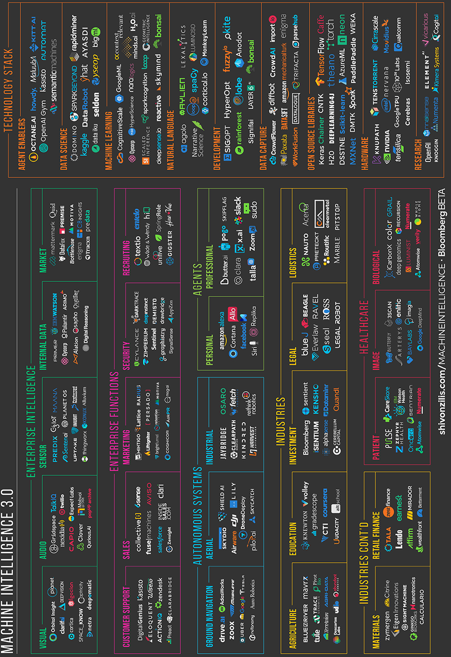
Figure 6-1. Machine intelligence landscape. Credit: Shivon Zilis and James Cham, designed by Heidi Skinner. (A larger version can be found on Shivon Zilis’ website.)
Ready Player World
Many of the most impressive-looking feats we’ve seen have been in the gaming world, from DeepMind beating Atari classics and the world’s best at Go, to the OpenAI gym, which allows anyone to train intelligent agents across an array of gaming environments.
The gaming world offers a perfect place to start machine intelligence work (e.g., constrained environments, explicit rewards, easy-to-compare results, looks impressive)—especially for reinforcement learning. And it is much easier to have a self-driving car agent go a trillion miles in a simulated environment than on actual roads. Now we’re seeing the techniques used to conquer the gaming world moving to the real world. A newsworthy example of game-tested technology entering the real world was when DeepMind used neural networks to make Google’s data centers more efficient. This begs questions: What else in the world looks like a game? Or what else in the world can we reconfigure to make it look more like a game?
Early attempts are intriguing. Developers are dodging meter maids (brilliant—a modern day Paper Boy), categorizing cucumbers, sorting trash, and recreating the memories of loved ones as conversational bots. Otto’s self-driving trucks delivering beer on their first commercial ride even seems like a bonus level from Grand Theft Auto. We’re excited to see what new creative applications come in the next year.
Why Even Bot-Her?
Ah, the great chatbot explosion of 2016, for better or worse—we liken it to the mobile app explosion we saw with the launch of iOS and Android. The dominant platforms (in the machine-intelligence case, Facebook, Slack, Kik) race to get developers to build on their platforms. That means we’ll get some excellent bots but also many terrible ones—the joys of public experimentation.
The danger here, unlike the mobile app explosion (where we lacked expectations for what these widgets could actually do), is that we assume anything with a conversation interface will converse with us at near-human level. Most do not. This is going to lead to disillusionment over the course of the next year, but it will clean itself up fairly quickly thereafter.
When our fund looks at this emerging field, we divide each technology into two components: the conversational interface itself and the “agent” behind the scenes that’s learning from data and transacting on a user’s behalf. While you certainly can’t drop the ball on the interface, we spend almost all our time thinking about that behind-the-scenes agent and whether it is actually solving a meaningful problem.
We get a lot of questions about whether there will be “one bot to rule them all.” To be honest, as with many areas at our fund, we disagree on this. We certainly believe there will not be one agent to rule them all, even if there is one interface to rule them all. For the time being, bots will be idiot savants: stellar for very specific applications.
We’ve written a bit about this, and the framework we use to think about how agents will evolve is a CEO and her support staff. Many Fortune 500 CEOs employ a scheduler, handler, a research team, a copy editor, a speechwriter, a personal shopper, a driver, and a professional coach. Each of these people performs a dramatically different function and has access to very different data to do their job. The bot/agent ecosystem will have a similar separation of responsibilities with very clear winners, and they will divide fairly cleanly along these lines. (Note that some CEOs have a chief of staff who coordinates among all these functions, so perhaps we will see examples of “one interface to rule them all.”)
You can also see, in our landscape, some of the corporate functions machine intelligence will reinvent (most often in interfaces other than conversational bots).
On to 11111000001
Successful use of machine intelligence at a large organization is surprisingly binary, like flipping a stubborn light switch. It’s hard to do, but once machine intelligence is enabled, an organization sees everything through the lens of its potential. Organizations like Google, Facebook, Apple, Microsoft, Amazon, Uber, and Bloomberg (our sole investor) bet heavily on machine intelligence and its capabilities are pervasive throughout all of their products.
Other companies are struggling to figure out what to do, as many boardrooms did on “what to do about the Internet” in 1997. Why is this so difficult for companies to wrap their heads around? Machine intelligence is different from traditional software. Unlike with big data, where you could buy a new capability, machine intelligence depends on deeper organizational and process changes. Companies need to decide whether they will trust machine-intelligence analysis for one-off decisions or if they will embed often-inscrutable machine-intelligence models in core processes. Teams need to figure out how to test newfound capabilities, and applications need to change so they offer more than a system of record; they also need to coach employees and learn from the data they enter.
Unlike traditional hardcoded software, machine intelligence gives only probabilistic outputs. We want to ask machine intelligence to make subjective decisions based on imperfect information (eerily like what we trust our colleagues to do?). As a result, this new machine-intelligence software will make mistakes, just like we do, and we’ll need to be thoughtful about when to trust it and when not to.
The idea of this new machine trust is daunting and makes machine intelligence harder to adopt than traditional software. We’ve had a few people tell us that the biggest predictor of whether a company will successfully adopt machine intelligence is whether it has a C-suite executive with an advanced math degree. These executives understand it isn’t magic—it is just (hard) math.
Machine-intelligence business models are going to be different from licensed and subscription software, but we don’t know how. Unlike traditional software, we still lack frameworks for management to decide where to deploy machine intelligence. Economists like Ajay Agrawal, Joshua Gans, and Avi Goldfarb have taken the first steps toward helping managers understand the economics of machine intelligence and predict where it will be most effective. But there is still a lot of work to be done.
In the next few years, the danger here isn’t what we see in dystopian sci-fi movies. The real danger of machine intelligence is that executives will make bad decisions about what machine-intelligence capabilities to build.
Peter Pan’s Never-Never Land
We’ve been wondering about the path to grow into a large machine-intelligence company. Unsurprisingly, there have been many machine-intelligence acquisitions (Nervana by Intel, Magic Pony by Twitter, Turi by Apple, Metamind by Salesforce, Otto by Uber, Cruise by GM, SalesPredict by Ebay, Viv by Samsung). Many of these happened fairly early in a company’s life and at quite a high price. Why is that?
Established companies struggle to understand machine-intelligence technology, so it’s painful to sell to them, and the market for buyers who can use this technology in a self-service way is small. Then, if you do understand how this technology can supercharge your organization, you realize it’s so valuable that you want to hoard it. Businesses are saying to machine-intelligence companies, “Forget you selling this technology to others; I’m going to buy the whole thing.”
This absence of a market today makes it difficult for a machine-intelligence startup, especially horizontal technology providers, to “grow up”—hence the Peter Pans. Companies we see successfully entering a long-term trajectory can package their technology as a new problem-specific application for enterprise or simply transform an industry themselves as a new entrant (love this). In this year’s landscape, we flagged a few of the industry categories where we believe startups might “go the distance.”
Inspirational Machine Intelligence
Once we do figure it out, machine-intelligence can solve much more interesting problems than traditional software. We’re thrilled to see so many smart people applying machine intelligence for good.
Established players like Conservation Metrics and Vulcan Conservation have been using deep learning to protect endangered animal species; the ever-inspiring team at Thorn is constantly coming up with creative algorithmic techniques to protect our children from online exploitation. The philanthropic arms of the tech titans joined in, enabling nonprofits with free storage, compute, and even developer time. Google partnered with nonprofits to found Global Fishing Watch to detect illegal fishing activity using satellite data in near real time, satellite intelligence startup Orbital Insight (in which we are investors) partnered with Global Forest Watch to detect illegal logging and other causes of global forest degradation. Startups are getting into the action, too. The Creative Destruction Lab machine intelligence accelerator (with whom we work closely) has companies working on problems like earlier disease detection and injury prevention. One area where we have seen some activity but would love to see more is machine intelligence to assist the elderly.
In talking to many people using machine intelligence for good, they all cite the critical role of open source technologies. In the last year, we’ve seen the launch of OpenAI, which offers everyone access to world-class research and environments, and better and better releases of TensorFlow and Keras. Nonprofits are always trying to do more with less, and machine intelligence has allowed them to extend the scope of their missions without extending budget. Algorithms allow nonprofits to inexpensively scale what would not be affordable to do with people.
We also saw growth in universities and corporate think tanks, where new centers like USC’s Center for AI in Society, Berkeley’s Center for Human Compatible AI, and the multiple-corporation Partnership on AI study the ways in which machine intelligence can help humanity. The White House even got into the act: after a series of workshops around the US, it published a 48-page report outlining its recommendations for applying machine intelligence to safely and fairly address broad social problems.
On a lighter note, we’ve also heard whispers of more artisanal versions of machine intelligence. Folks are doing things like using computer vision algorithms to help them choose the best cocoa beans for high-grade chocolate, write poetry, cook steaks, and generate musicals.
Curious minds want to know. If you’re working on a unique or important application of machine intelligence, we’d love to hear from you.
Looking Forward
We see all this activity only continuing to accelerate. The world will give us more open sourced and commercially available machine-intelligence building blocks, there will be more data, there will be more people interested in learning these methods, and there will always be problems worth solving. We still need ways of explaining the difference between machine intelligence and traditional software, and we’re working on that. The value of code is different from data, but what about the value of the model that code improves based on that data?
Once we understand machine intelligence deeply, we might look back on the era of traditional software and think it was just a prologue to what’s happening now. We look forward to seeing what the next year brings.
Hello, TensorFlow!
You can read this post on oreilly.com here.
The TensorFlow project is bigger than you might realize. The fact that it’s a library for deep learning and its connection to Google, have helped TensorFlow attract a lot of attention. But beyond the hype, there are unique elements to the project that are worthy of closer inspection:
- The core library is suited to a broad family of machine-learning techniques, not “just” deep learning.
- Linear algebra and other internals are prominently exposed.
- In addition to the core machine-learning functionality, TensorFlow also includes its own logging system, its own interactive log visualizer, and even its own heavily engineered serving architecture.
- The execution model for TensorFlow differs from Python’s scikit-learn, and most tools in R.
Cool stuff, but—especially for someone hoping to explore machine learning for the first time—TensorFlow can be a lot to take in.
How does TensorFlow work? Let’s break it down so we can see and understand every moving part. We’ll explore the data flow graph that defines the computations your data will undergo, how to train models with gradient descent using TensorFlow, and how TensorBoard can visualize your TensorFlow work. The examples here won’t solve industrial machine-learning problems, but they’ll help you understand the components underlying everything built with TensorFlow, including whatever you build next!
Names and Execution in Python and TensorFlow
The way TensorFlow manages computation is not totally different from the way Python usually does. With both, it’s important to remember, to paraphrase Hadley Wickham, that an object has no name (see Figure 6-2). In order to see the similarities (and differences) between how Python and TensorFlow work, let’s look at how they refer to objects and handle evaluation.

Figure 6-2. Names “have” objects, rather than the reverse. Credit: Hadley Wickham. Used with permission.
The variable names in Python code aren’t what they represent; they’re just pointing at objects. So, when you say in Python that foo = [] and bar = foo, it isn’t just that foo equals bar; foo is bar, in the sense that they both point at the same list object:
>>> foo = []
>>> bar = foo
>>> foo == bar
## True
>>> foo is bar
## True
You can also see that id(foo) and id(bar) are the same. This identity, especially with mutable data structures like lists, can lead to surprising bugs when it’s misunderstood.
Internally, Python manages all your objects and keeps track of your variable names and which objects they refer to. The TensorFlow graph represents another layer of this kind of management; as we’ll see, Python names will refer to objects that connect to more granular and managed TensorFlow graph operations.
When you enter a Python expression, for example at an interactive interpreter or Read-Evaluate-Print-Loop (REPL), whatever is read is almost always evaluated right away. Python is eager to do what you tell it. So, if I tell Python to foo.append(bar), it appends right away, even if I never use foo again.
A lazier alternative would be to just remember that I said foo.append(bar), and if I ever evaluate foo at some point in the future, Python could do the append then. This would be closer to how TensorFlow behaves, where defining relationships is entirely separate from evaluating what the results are.
TensorFlow separates the definition of computations from their execution even further by having them happen in separate places: a graph defines the operations, but the operations only happen within a session. Graphs and sessions are created independently. A graph is like a blueprint, and a session is like a construction site.
Back to our plain Python example, recall that foo and bar refer to the same list. By appending bar into foo, we’ve put a list inside itself. You could think of this structure as a graph with one node, pointing to itself. Nesting lists is one way to represent a graph structure like a TensorFlow computation graph:
>>>foo.append(bar)>>>foo## [[...]]
Real TensorFlow graphs will be more interesting than this!
The Simplest TensorFlow Graph
To start getting our hands dirty, let’s create the simplest TensorFlow graph we can, from the ground up. TensorFlow is admirably easier to install than some other frameworks. The examples here work with either Python 2.7 or 3.3+, and the TensorFlow version used is 0.8:
>>>importtensorflowastf
At this point, TensorFlow has already started managing a lot of state for us. There’s already an implicit default graph, for example. Internally, the default graph lives in the _default_graph_stack, but we don’t have access to that directly. We use tf.get_default_graph():
>>>graph=tf.get_default_graph()
The nodes of the TensorFlow graph are called “operations,” or “ops.” We can see what operations are in the graph with graph.get_operations():
>>>graph.get_operations()## []
Currently, there isn’t anything in the graph. We’ll need to put everything we want TensorFlow to compute into that graph. Let’s start with a simple constant input value of 1:
>>>input_value=tf.constant(1.0)
That constant now lives as a node, an operation, in the graph. The Python variable name input_value refers indirectly to that operation, but we can also find the operation in the default graph:
>>>operations=graph.get_operations()>>>operations## [<tensorflow.python.framework.ops.Operation at 0x1185005d0>]>>>operations[0].node_def## name: "Const"## op: "Const"## attr {## key: "dtype"## value {## type: DT_FLOAT## }## }## attr {## key: "value"## value {## tensor {## dtype: DT_FLOAT## tensor_shape {## }## float_val: 1.0## }## }## }
TensorFlow uses protocol buffers internally. (Protocol buffers are sort of like a Google-strength JSON.) Printing the node_def for the constant operation in the preceding code block shows what’s in TensorFlow’s protocol buffer representation for the number 1.
People new to TensorFlow sometimes wonder why there’s all this fuss about making “TensorFlow versions” of things. Why can’t we just use a normal Python variable without also defining a TensorFlow object? One of the TensorFlow tutorials has an explanation:
To do efficient numerical computing in Python, we typically use libraries like NumPy that do expensive operations such as matrix multiplication outside Python, using highly efficient code implemented in another language. Unfortunately, there can still be a lot of overhead from switching back to Python every operation. This overhead is especially bad if you want to run computations on GPUs or in a distributed manner, where there can be a high cost to transferring data.
TensorFlow also does its heavy lifting outside Python, but it takes things a step further to avoid this overhead. Instead of running a single expensive operation independently from Python, TensorFlow lets us describe a graph of interacting operations that run entirely outside Python. This approach is similar to that used in Theano or Torch.
TensorFlow can do a lot of great things, but it can only work with what’s been explicitly given to it. This is true even for a single constant.
If we inspect our input_value, we see it is a constant 32-bit float tensor of no dimension: just one number:
>>>input_value## <tf.Tensor 'Const:0' shape=() dtype=float32>
Note that this doesn’t tell us what that number is. To evaluate input_value and get a numerical value out, we need to create a “session” where graph operations can be evaluated and then explicitly ask to evaluate or “run” input_value. (The session picks up the default graph by default.)
>>>sess=tf.Session()>>>sess.run(input_value)## 1.0
It may feel a little strange to “run” a constant. But it isn’t so different from evaluating an expression as usual in Python; it’s just that TensorFlow is managing its own space of things—the computational graph—and it has its own method of evaluation.
The Simplest TensorFlow Neuron
Now that we have a session with a simple graph, let’s build a neuron with just one parameter, or weight. Often, even simple neurons also have a bias term and a nonidentity activation function, but we’ll leave these out.
The neuron’s weight isn’t going to be constant; we expect it to change in order to learn based on the “true” input and output we use for training. The weight will be a TensorFlow variable. We’ll give that variable a starting value of 0.8:
>>>weight=tf.Variable(0.8)
You might expect that adding a variable would add one operation to the graph, but in fact that one line adds four operations. We can check all the operation names:
>>>foropingraph.get_operations():(op.name)## Const## Variable/initial_value## Variable## Variable/Assign## Variable/read
We won’t want to follow every operation individually for long, but it will be nice to see at least one that feels like a real computation:
>>>output_value=weight*input_value
Now there are six operations in the graph, and the last one is that multiplication:
>>>op=graph.get_operations()[-1]>>>op.name## 'mul'>>>forop_inputinop.inputs:(op_input)## Tensor("Variable/read:0", shape=(), dtype=float32)## Tensor("Const:0", shape=(), dtype=float32)
This shows how the multiplication operation tracks where its inputs come from: they come from other operations in the graph. To understand a whole graph, following references this way quickly becomes tedious for humans. TensorBoard graph visualization is designed to help.
How do we find out what the product is? We have to “run” the output_value operation. But that operation depends on a variable: weight. We told TensorFlow that the initial value of weight should be 0.8, but the value hasn’t yet been set in the current session. The tf.initialize_all_variables() function generates an operation which will initialize all our variables (in this case just one), and then we can run that operation:
>>>init=tf.initialize_all_variables()>>>sess.run(init)
The result of tf.initialize_all_variables() will include initializers for all the variables currently in the graph, so if you add more variables you’ll want to use tf.initialize_all_variables() again; a stale init wouldn’t include the new variables.
Now we’re ready to run the output_value operation:
>>>sess.run(output_value)## 0.80000001
Recall that it is 0.8 * 1.0 with 32-bit floats, and 32-bit floats have a hard time with 0.8; 0.80000001 is as close as they can get.
See Your Graph in TensorBoard
Up to this point, the graph has been simple, but it would already be nice to see it represented in a diagram. We’ll use TensorBoard to generate that diagram. TensorBoard reads the name field that is stored inside each operation (quite distinct from Python variable names). We can use these TensorFlow names and switch to more conventional Python variable names. Using tf.mul here is equivalent to our earlier use of just * for multiplication, but it lets us set the name for the operation:
>>>x=tf.constant(1.0,name='input')>>>w=tf.Variable(0.8,name='weight')>>>y=tf.mul(w,x,name='output')
TensorBoard works by looking at a directory of output created from TensorFlow sessions. We can write this output with a SummaryWriter, and if we do nothing aside from creating one with a graph, it will just write out that graph.
The first argument when creating the SummaryWriter is an output directory name, which will be created if it doesn’t exist:
>>>summary_writer=tf.train.SummaryWriter('log_simple_graph',sess.graph)
Now, at the command line, we can start up TensorBoard:
$ tensorboard --logdir=log_simple_graph
TensorBoard runs as a local web app, on port 6006. (“6006” is “goog” upside-down.) If you go in a browser to localhost:6006/#graphs, you should see a diagram of the graph you created in TensorFlow, which looks something like Figure 6-3.

Figure 6-3. A TensorBoard visualization of the simplest TensorFlow neuron.
Making the Neuron Learn
Now that we’ve built our neuron, how does it learn? We set up an input value of 1.0. Let’s say the correct output value is zero. That is, we have a very simple “training set” of just one example with one feature, which has the value 1, and one label, which is zero. We want the neuron to learn the function taking 1 to 0.
Currently, the system takes the input 1 and returns 0.8, which is not correct. We need a way to measure how wrong the system is. We’ll call that measure of wrongness the “loss” and give our system the goal of minimizing the loss. If the loss can be negative, then minimizing it could be silly, so let’s make the loss the square of the difference between the current output and the desired output:
>>>y_=tf.constant(0.0)>>>loss=(y-y_)**2
So far, nothing in the graph does any learning. For that, we need an optimizer. We’ll use a gradient descent optimizer so that we can update the weight based on the derivative of the loss. The optimizer takes a learning rate to moderate the size of the updates, which we’ll set at 0.025:
>>>optim=tf.train.GradientDescentOptimizer(learning_rate=0.025)
The optimizer is remarkably clever. It can automatically work out and apply the appropriate gradients through a whole network, carrying out the backward step for learning.
Let’s see what the gradient looks like for our simple example:
>>>grads_and_vars=optim.compute_gradients(loss)>>>sess.run(tf.initialize_all_variables())>>>sess.run(grads_and_vars[1][0])## 1.6
Why is the value of the gradient 1.6? Our loss is error squared, and the derivative of that is two times the error. Currently the system says 0.8 instead of 0, so the error is 0.8, and two times 0.8 is 1.6. It’s working!
For more complex systems, it will be very nice indeed that TensorFlow calculates and then applies these gradients for us automatically.
Let’s apply the gradient, finishing the backpropagation:
>>>sess.run(optim.apply_gradients(grads_and_vars))>>>sess.run(w)## 0.75999999 # about 0.76
The weight decreased by 0.04 because the optimizer subtracted the gradient times the learning rate, 1.6 * 0.025, pushing the weight in the right direction.
Instead of hand-holding the optimizer like this, we can make one operation that calculates and applies the gradients: the train_step:
>>>train_step=tf.train.GradientDescentOptimizer(0.025).minimize(loss)>>>foriinrange(100):>>>sess.run(train_step)>>>>>>sess.run(y)## 0.0044996012
Running the training step many times, the weight and the output value are now very close to zero. The neuron has learned!
Training diagnostics in TensorBoard
We may be interested in what’s happening during training. Say we want to follow what our system is predicting at every training step. We could print from inside the training loop:
>>>sess.run(tf.initialize_all_variables())>>>foriinrange(100):>>>('before step {}, y is {}'.format(i,sess.run(y)))>>>sess.run(train_step)>>>## before step 0, y is 0.800000011921## before step 1, y is 0.759999990463## ...## before step 98, y is 0.00524811353534## before step 99, y is 0.00498570781201
This works, but there are some problems. It’s hard to understand a list of numbers. A plot would be better. And even with only one value to monitor, there’s too much output to read. We’re likely to want to monitor many things. It would be nice to record everything in some organized way.
Luckily, the same system that we used earlier to visualize the graph also has just the mechanisms we need.
We instrument the computation graph by adding operations that summarize its state. Here, we’ll create an operation that reports the current value of y, the neuron’s current output:
>>>summary_y=tf.scalar_summary('output',y)
When you run a summary operation, it returns a string of protocol buffer text that can be written to a log directory with a SummaryWriter:
>>>summary_writer=tf.train.SummaryWriter('log_simple_stats')>>>sess.run(tf.initialize_all_variables())>>>foriinrange(100):>>>summary_str=sess.run(summary_y)>>>summary_writer.add_summary(summary_str,i)>>>sess.run(train_step)>>>
Now after running tensorboard --logdir=log_simple_stats, you get an interactive plot at localhost:6006/#events (Figure 6-4).

Figure 6-4. A TensorBoard visualization of a neuron’s output against training iteration number.
Flowing Onward
Here’s a final version of the code. It’s fairly minimal, with every part showing useful (and understandable) TensorFlow functionality:
importtensorflowastfx=tf.constant(1.0,name='input')w=tf.Variable(0.8,name='weight')y=tf.mul(w,x,name='output')y_=tf.constant(0.0,name='correct_value')loss=tf.pow(y-y_,2,name='loss')train_step=tf.train.GradientDescentOptimizer(0.025).minimize(loss)forvaluein[x,w,y,y_,loss]:tf.scalar_summary(value.op.name,value)summaries=tf.merge_all_summaries()sess=tf.Session()summary_writer=tf.train.SummaryWriter('log_simple_stats',sess.graph)sess.run(tf.initialize_all_variables())foriinrange(100):summary_writer.add_summary(sess.run(summaries),i)sess.run(train_step)
The example we just ran through is even simpler than the ones that inspired it in Michael Nielsen’s Neural Networks and Deep Learning. For myself, seeing details like these helps with understanding and building more complex systems that use and extend from simple building blocks. Part of the beauty of TensorFlow is how flexibly you can build complex systems from simpler components.
If you want to continue experimenting with TensorFlow, it might be fun to start making more interesting neurons, perhaps with different activation functions. You could train with more interesting data. You could add more neurons. You could add more layers. You could dive into more complex prebuilt models, or spend more time with TensorFlow’s own tutorials and how-to guides. Go for it!
Compressing and Regularizing Deep Neural Networks
You can read this post on oreilly.com here.
Deep neural networks have evolved to be the state-of-the-art technique for machine-learning tasks ranging from computer vision and speech recognition to natural language processing. However, deep-learning algorithms are both computationally intensive and memory intensive, making them difficult to deploy on embedded systems with limited hardware resources.
To address this limitation, deep compression significantly reduces the computation and storage required by neural networks. For example, for a convolutional neural network with fully connected layers, such as Alexnet and VGGnet, it can reduce the model size by 35x–49x. Even for fully convolutional neural networks such as GoogleNet and SqueezeNet, deep compression can still reduce the model size by 10x. Both scenarios results in no loss of prediction accuracy.
Current Training Methods Are Inadequate
Compression without losing accuracy means there’s significant redundancy in the trained model, which shows the inadequacy of current training methods. To address this, I’ve worked with Jeff Pool, of NVIDIA, Sharan Narang of Baidu, and Peter Vajda of Facebook to develop the dense-sparse-dense (DSD) training, a novel training method that first regularizes the model through sparsity-constrained optimization, and improves the prediction accuracy by recovering and retraining on pruned weights. At test time, the final model produced by DSD training still has the same architecture and dimension as the original dense model, and DSD training doesn’t incur any inference overhead. We experimented with DSD training on mainstream CNN/RNN/LSTMs for image classification, image caption, and speech recognition and found substantial performance improvements.
In this article, we first introduce deep compression, and then introduce dense-sparse-dense training.
Deep Compression
The first step of deep compression is synaptic pruning. The human brain inherently has the process of pruning. 5x synapses are pruned away from infant age to adulthood.
Does a similar process occur in artificial neural networks? The answer is yes. In early work, network pruning proved to be a valid way to reduce the network complexity and overfitting. This method works on modern neural networks as well. We start by learning the connectivity via normal network training. Next, we prune the small-weight connections: all connections with weights below a threshold are removed from the network. Finally, we retrain the network to learn the final weights for the remaining sparse connections. Pruning reduced the number of parameters by 9x and 13x for AlexNet and the VGG-16 model, respectively.
The next step of deep compression is weight sharing. We found neural networks have a really high tolerance for low precision: aggressive approximation of the weight values does not hurt the prediction accuracy. As shown in Figure 6-6, the blue weights are originally 2.09, 2.12, 1.92 and 1.87; by letting four of them share the same value, which is 2.00, the accuracy of the network can still be recovered. Thus we can save very few weights, call it “codebook,” and let many other weights share the same weight, storing only the index to the codebook.

Figure 6-5. Pruning a neural network. Credit: Song Han.
The index could be represented with very few bits; for example, in Figure 6-6, there are four colors; thus only two bits are needed to represent a weight as opposed to 32 bits originally. The codebook, on the other side, occupies negligible storage. Our experiments found this kind of weight-sharing technique is better than linear quantization, with respect to the compression ratio and accuracy trade-off.

Figure 6-6. Training a weight-sharing neural network.
Figure 6-7 shows the overall result of deep compression. Lenet-300-100 and Lenet-5 are evaluated on a MNIST data set, while AlexNet, VGGNet, GoogleNet, and SqueezeNet are evaluated on an ImageNet data set. The compression ratio ranges from 10x to 49x—even for those fully convolutional neural networks like GoogleNet and SqueezeNet, deep compression can still compress it by an order of magnitude. We highlight SqueezeNet, which has 50x fewer parameters than AlexNet but has the same accuracy, and can still be compressed by 10x, making it only 470 KB. This makes it easy to fit in on-chip SRAM, which is both faster and more energy-efficient to access than DRAM.
We have tried other compression methods such as low-rank approximation-based methods, but the compression ratio isn’t as high. A complete discussion can be found in the “Deep Compression” paper.

Figure 6-7. Results of deep compression.
DSD Training
The fact that deep neural networks can be aggressively pruned and compressed means that our current training method has some limitation: it can not fully exploit the full capacity of the dense model to find the best local minima; yet a pruned, sparse model that has much fewer synapses can achieve the same accuracy. This raises a question: can we achieve better accuracy by recovering those weights, and learn them again?
Let’s make an analogy to training for track racing in the Olympics. The coach will first train a runner on high-altitude mountains, where there are a lot of constraints: low oxygen, cold weather, etc. The result is that when the runner returns to the plateau area again, his/her speed is increased. Similar for neural networks, given the heavily constrained sparse training, the network performs as well as the dense model; once you release the constraint, the model can work better.
Theoretically, the following factors contribute to the effectiveness of DSD training:
- Escape saddle point: one of the most profound difficulties of optimizing deep networks is the proliferation of saddle points. DSD training overcomes saddle points by a pruning and re-densing framework. Pruning the converged model perturbs the learning dynamics and allows the network to jump away from saddle points, which gives the network a chance to converge at a better local or global minimum. This idea is also similar to simulated annealing. While simulated annealing randomly jumps with decreasing probability on the search graph, DSD deterministically deviates from the converged solution achieved in the first dense training phase by removing the small weights and enforcing a sparsity support.
- Regularized and sparse training: the sparsity regularization in the sparse training step moves the optimization to a lower-dimensional space where the loss surface is smoother and tends to be more robust to noise. More numerical experiments verified that both sparse training and the final DSD reduce the variance and lead to lower error.
- Robust reinitialization: weight initialization plays a big role in deep learning. Conventional training has only one chance of initialization. DSD gives the optimization a second (or more) chance during the training process to reinitialize from more robust sparse training solutions. We re-dense the network from the sparse solution, which can be seen as a zero initialization for pruned weights. Other initialization methods are also worth trying.
- Break symmetry: The permutation symmetry of the hidden units makes the weights symmetrical, thus prone to co-adaptation in training. In DSD, pruning the weights breaks the symmetry of the hidden units associated with the weights, and the weights are asymmetrical in the final dense phase.
We examined several mainstream CNN/RNN/LSTM architectures on image classification, image caption, and speech recognition data sets, and found that this dense-sparse-dense training flow gives significant accuracy improvement. Our DSD training employs a three-step process: dense, sparse, dense; each step is illustrated in Figure 6-8:

Figure 6-8. Dense-sparse-dense training flow.
- Initial dense training: the first D-step learns the connectivity via normal network training on the dense network. Unlike conventional training, however, the goal of this D step is not to learn the final values of the weights; rather, we are learning which connections are important.
- Sparse training: the S-step prunes the low-weight connections and retrains the sparse network. We applied the same sparsity to all the layers in our experiments; thus there’s a single hyperparameter: the sparsity. For each layer, we sort the parameters, and the smallest N*sparsity parameters are removed from the network, converting a dense network into a sparse network. We found that a sparsity ratio of 50%–70% works very well. Then, we retrain the sparse network, which can fully recover the model accuracy under the sparsity constraint.
- Final dense training: the final D step recovers the pruned connections, making the network dense again. These previously pruned connections are initialized to zero and retrained. Restoring the pruned connections increases the dimensionality of the network, and more parameters make it easier for the network to slide down the saddle point to arrive at a better local minima.
We applied DSD training to different kinds of neural networks on data sets from different domains. We found that DSD training improved the accuracy for all these networks compared to neural networks that were not trained with DSD. The neural networks are chosen from CNN, RNN, and LSTMs; the data sets are chosen from image classification, speech recognition, and caption generation. The results are shown in Figure 6-9. DSD models are available to download at DSD Model Zoo.

Figure 6-9. DSD training improves the prediction accuracy.
Generating Image Descriptions
We visualized the effect of DSD training on an image caption task (see Figure 6-10). We applied DSD to NeuralTalk, an LSTM for generating image descriptions. The baseline model fails to describe images 1, 4, and 5. For example, in the first image, the baseline model mistakes the girl for a boy, and mistakes the girl’s hair for a rock wall; the sparse model can tell that it’s a girl in the image, and the DSD model can further identify the swing.
In the the second image, DSD training can tell that the player is trying to make a shot, rather than the baseline, which just says he’s playing with a ball. It’s interesting to notice that the sparse model sometimes works better than the DSD model. In the last image, the sparse model correctly captured the mud puddle, while the DSD model only captured the forest from the background. The good performance of DSD training generalizes beyond these examples, and more image caption results generated by DSD training are provided in the appendix of this paper.

Figure 6-10. Visualization of DSD training improves the performance of image captioning.
Advantages of Sparsity
Deep compression for compressing deep neural networks for smaller model size and DSD training for regularizing neural networks are techniques that utilize sparsity and achieve a smaller size or higher prediction accuracy. Apart from model size and prediction accuracy, we looked at two other dimensions that take advantage of sparsity: speed and energy efficiency, which is beyond the scope of this article. Readers can refer to our paper “EIE: Efficient Inference Engine on Compressed Deep Neural Network” for further references.