Watermarks

Watermarks are the first half of the answer to the question: “When in processing time are results materialized?” Watermarks are temporal notions of input completeness in the event-time domain. Worded differently, they are the way the system measures progress and completeness relative to the event times of the records being processed in a stream of events (either bounded or unbounded, though their usefulness is more apparent in the unbounded case).

Recall this diagram from “Streaming 101,” slightly modified here, where I described the skew between event time and processing time as an ever-changing function of time for most real-world distributed data processing systems (Figure 3-1).

Figure 3-1. Event time progress, skew, and watermarks. Credit: Tyler Akidau.

That meandering red line that I claimed represented reality is essentially the watermark; it captures the progress of event time completeness as processing time progresses. Conceptually, you can think of the watermark as a function, F(P) → E, which takes a point in processing time and returns a point in event time. (More accurately, the input to the function is really the current state of everything upstream of the point in the pipeline where the watermark is being observed: the input source, buffered data, data actively being processed, etc. But conceptually, it’s simpler to think of it as a mapping from processing time to event time.) That point in event time, E, is the point up to which the system believes all inputs with event times less than E have been observed. In other words, it’s an assertion that no more data with event times less than E will ever be seen again. Depending upon the type of watermark, perfect or heuristic, that assertion may be a strict guarantee or an educated guess, respectively:

• Perfect watermarks: in the case where we have perfect knowledge of all of the input data, it’s possible to construct a perfect watermark. In such a case, there is no such thing as late data; all data are early or on time.
• Heuristic watermarks: for many distributed input sources, perfect knowledge of the input data is impractical, in which case the next best option is to provide a heuristic watermark. Heuristic watermarks use whatever information is available about the inputs (partitions, ordering within partitions if any, growth rates of files, etc.) to provide an estimate of progress that is as accurate as possible. In many cases, such watermarks can be remarkably accurate in their predictions. Even so, the use of a heuristic watermark means it may sometimes be wrong, which will lead to late data. We’ll learn about ways to deal with late data in “The wonderful thing about triggers, is triggers are wonderful things!”.

Watermarks are a fascinating and complex topic, with far more to talk about than I can reasonably fit here or in the margin, so a further deep dive on them will have to wait for a future post. For now, to get a better sense of the role that watermarks play, as well as some of their shortcomings, let’s look at two examples of a streaming engine using watermarks alone to determine when to materialize output while executing the windowed pipeline from Listing 2. The example in Figure 3-2 uses a perfect watermark; the one in Figure 3-3 uses a heuristic watermark.

Figure 3-2. Windowed summation on a streaming engine with perfect watermarks. Credit: Tyler Akidau.

Figure 3-3. Windowed summation on a streaming engine with heuristic watermarks. Credit: Tyler Akidau.

In both cases, windows are materialized as the watermark passes the end of the window. The primary difference between the two executions is that the heuristic algorithm used in watermark calculation on the right fails to take the value of 9 into account, which drastically changes the shape of the watermark. These examples highlight two shortcomings of watermarks (and any other notion of completeness), specifically that they can be:

• Too slow: when a watermark of any type is correctly delayed due to known unprocessed data (e.g., slowly growing input logs due to network bandwidth constraints), that translates directly into delays in output if advancement of the watermark is the only thing you depend on for stimulating results.

  This is most obvious in Figure 3-2, where the late-arriving 9 holds back the watermark for all the subsequent windows, even though the input data for those windows become complete earlier. This is particularly apparent for the second window, (12:02, 12:04), where it takes nearly seven minutes from the time the first value in the window occurs until we see any results for the window whatsoever. The heuristic watermark in this example doesn’t suffer the same issue quite so badly (five minutes until output), but don’t take that to mean heuristic watermarks never suffer from watermark lag; that’s really just a consequence of the record I chose to omit from the heuristic watermark in this specific example.

  The important point here is the following: while watermarks provide a very useful notion of completeness, depending upon completeness for producing output is often not ideal from a latency perspective. Imagine a dashboard that contains valuable metrics, windowed by hour or day. It’s unlikely that you’d want to wait a full hour or day to begin seeing results for the current window; that’s one of the pain points of using classic batch systems to power such systems. Instead, it would be much nicer to see the results for those windows refine over time as the inputs evolve and eventually become complete.

• Too fast: when a heuristic watermark is incorrectly advanced earlier than it should be, it’s possible for data with event times before the watermark to arrive some time later, creating late data. This is what happened in the example in Figure 3-3: the watermark advanced past the end of the first window before all the input data for that window had been observed, resulting in an incorrect output value of 5 instead of 14. This shortcoming is strictly a problem with heuristic watermarks; their heuristic nature implies they will sometimes be wrong. As a result, relying on them alone for determining when to materialize output is insufficient if you care about correctness.

In “Streaming 101,” I made some rather emphatic statements about notions of completeness being insufficient for robust out-of-order processing of unbounded data streams. These two shortcomings, watermarks being too slow or too fast, are the foundations for those arguments. You simply cannot get both low latency and correctness out of a system that relies solely on notions of completeness. Addressing these shortcomings is where triggers come into play.

The wonderful thing about triggers, is triggers are wonderful things!

Triggers are the second half of the answer to the question: “When in processing time are results materialized?” Triggers declare when output for a window should happen in processing time (though the triggers themselves may make those decisions based off of things that happen in other time domains, such as watermarks progressing in the event-time domain). Each specific output for a window is referred to as a pane of the window.

Examples of signals used for triggering include:

• Watermark progress (i.e., event-time progress), an implicit version of which we already saw in Figures 3-2 and 3-3, where outputs were materialized when the watermark passed the end of the window.¹ Another use case is triggering garbage collection when the lifetime of a window exceeds some useful horizon, an example of which we’ll see a little later on.

• Processing time progress, which is useful for providing regular, periodic updates because processing time (unlike event time) always progresses more or less uniformly and without delay.

• Element counts, which are useful for triggering after some finite number of elements have been observed in a window.

• Punctuations, or other data-dependent triggers, where some record or feature of a record (e.g., an EOF element or a flush event) indicates that output should be generated.

In addition to simple triggers that fire based off of concrete signals, there are also composite triggers that allow for the creation of more sophisticated triggering logic. Example composite triggers include:

• Repetitions, which are particularly useful in conjunction with processing time triggers for providing regular, periodic updates.
• Conjunctions (logical AND), which fire only once all child triggers have fired (e.g., after the watermark passes the end of the window AND we observe a terminating punctuation record).
• Disjunctions (logical OR), which fire after any child triggers fire (e.g., after the watermark passes the end of the window OR we observe a terminating punctuation record).
• Sequences, which fire a progression of child triggers in a predefined order.

To make the notion of triggers a bit more concrete (and give us something to build upon), let’s go ahead and make explicit the implicit default trigger used in 3-2 and 3-3 by adding it to the code from Listing 2.

PCollection<KV<String, Integer>> scores = input
  .apply(Window.into(FixedWindows.of(Duration.standardMinutes(2)))
               .triggering(AtWatermark()))
  .apply(Sum.integersPerKey());

With that in mind, and a basic understanding of what triggers have to offer, we can look at tackling the problems of watermarks being too slow or too fast. In both cases, we essentially want to provide some sort of regular, materialized updates for a given window, either before or after the watermark advances past the end of the window (in addition to the update we’ll receive at the threshold of the watermark passing the end of the window). So, we’ll want some sort of repetition trigger. The question then becomes: what are we repeating?

In the “too slow” case (i.e., providing early, speculative results), we probably should assume that there may be a steady amount of incoming data for any given window because we know (by definition of being in the early stage for the window) that the input we’ve observed for the window is thus far incomplete. As such, triggering periodically when processing time advances (e.g., once per minute) is probably wise because the number of trigger firings won’t be dependent upon the amount of data actually observed for the window; at worst, we’ll just get a steady flow of periodic trigger firings.

In the “too fast” case (i.e., providing updated results in response to late data due to a heuristic watermark), let’s assume our watermark is based on a relatively accurate heuristic (often a reasonably safe assumption). In that case, we don’t expect to see late data very often, but when we do, it would be nice to amend our results quickly. Triggering after observing an element count of 1 will give us quick updates to our results (i.e., immediately any time we see late data), but is not likely to overwhelm the system, given the expected infrequency of late data.

Note that these are just examples: we’re free to choose different triggers (or to choose not to trigger at all for one or both of them) if appropriate for the use case at hand.

Lastly, we need to orchestrate the timing of these various triggers: early, on-time, and late. We can do this with a Sequence trigger and a special OrFinally trigger, which installs a child trigger that terminates the parent trigger when the child fires.

PCollection<KV<String, Integer>> scores = input
  .apply(Window.into(FixedWindows.of(Duration.standardMinutes(2)))
               .triggering(Sequence(
                 Repeat(AtPeriod(Duration.standardMinutes(1)))
                   .OrFinally(AtWatermark()),
                 Repeat(AtCount(1))))
  .apply(Sum.integersPerKey());

However, that’s pretty wordy. And given that the pattern of repeated-early | on-time | repeated-late firings is so common, we provide a custom (but semantically equivalent) API in Dataflow to make specifying such triggers simpler and clearer:

PCollection<KV<String, Integer>> scores = input
  .apply(Window.into(FixedWindows.of(Duration.standardMinutes(2)))
               .triggering(
                 AtWatermark()
                   .withEarlyFirings(AtPeriod(Duration
                   .standardMinutes(1)))
                   .withLateFirings(AtCount(1))))
  .apply(Sum.integersPerKey());

Executing either Listing 4 or 5 on a streaming engine (with both perfect and heuristic watermarks, as before) then yields results that look like Figures 3-4 and 3-5.

Figure 3-4. Windowed summation on a streaming engine with early and late firings (perfect watermark). Credit: Tyler Akidau.

Figure 3-5. Windowed summation on a streaming engine with early and late firings (heuristic watermark). Credit: Tyler Akidau.

This version has two clear improvements over Figures 3-2 and 3-3:

• For the “watermarks too slow” case in the second window, (12:02, 12:04): we now provide periodic early updates once per minute. The difference is most stark in the perfect watermark case, where time-to-first-output is reduced from almost seven minutes down to three and a half; but it’s also clearly improved in the heuristic case as well. Both versions now provide steady refinements over time (panes with values 7, 14, then 22), with relatively minimal latency between the input becoming complete and materialization of the final output pane for the window.

• For the “heuristic watermarks too fast” case in the first window, (12:00, 12:02): when the value of 9 shows up late, we immediately incorporate it into a new, corrected pane with a value of 14.

One interesting side effect of these new triggers is that they effectively normalize the output pattern between the perfect and heuristic watermark versions. Whereas the two versions in Figures 3-2 and 3-3 were starkly different, the two versions here look quite similar.

The biggest remaining difference at this point is window lifetime bounds. In the perfect watermark case, we know we’ll never see any more data for a window once the watermark has passed the end of it; hence we can drop all of our state for the window at that time. In the heuristic watermark case, we still need to hold on to the state for a window for some amount of time to account for late data. But as of yet, our system doesn’t have any good way of knowing just how long state needs to be kept around for each window. That’s where allowed lateness comes in. 

Increased efficiency

Incrementally processing new data in “mini” batches could be a much more efficient use of resources for the organization. Let’s take a concrete example, where we have a stream of Kafka events coming in at 10K/sec and we want to count the number of messages in the last 15 minutes across some dimensions. Most stream-processing pipelines use an external result store (e.g., Cassandra, ElasticSearch) to keep aggregating the count, and keep the YARN/Mesos containers running the whole time. This makes sense in the less-than-five-minute latency windows such pipelines operate on. In practice, typical YARN container start-up costs tend to be around a minute. In addition, to scale the writes to the result stores, we often end up buffering and batching updates, and this protocol needs the containers to be long-running.

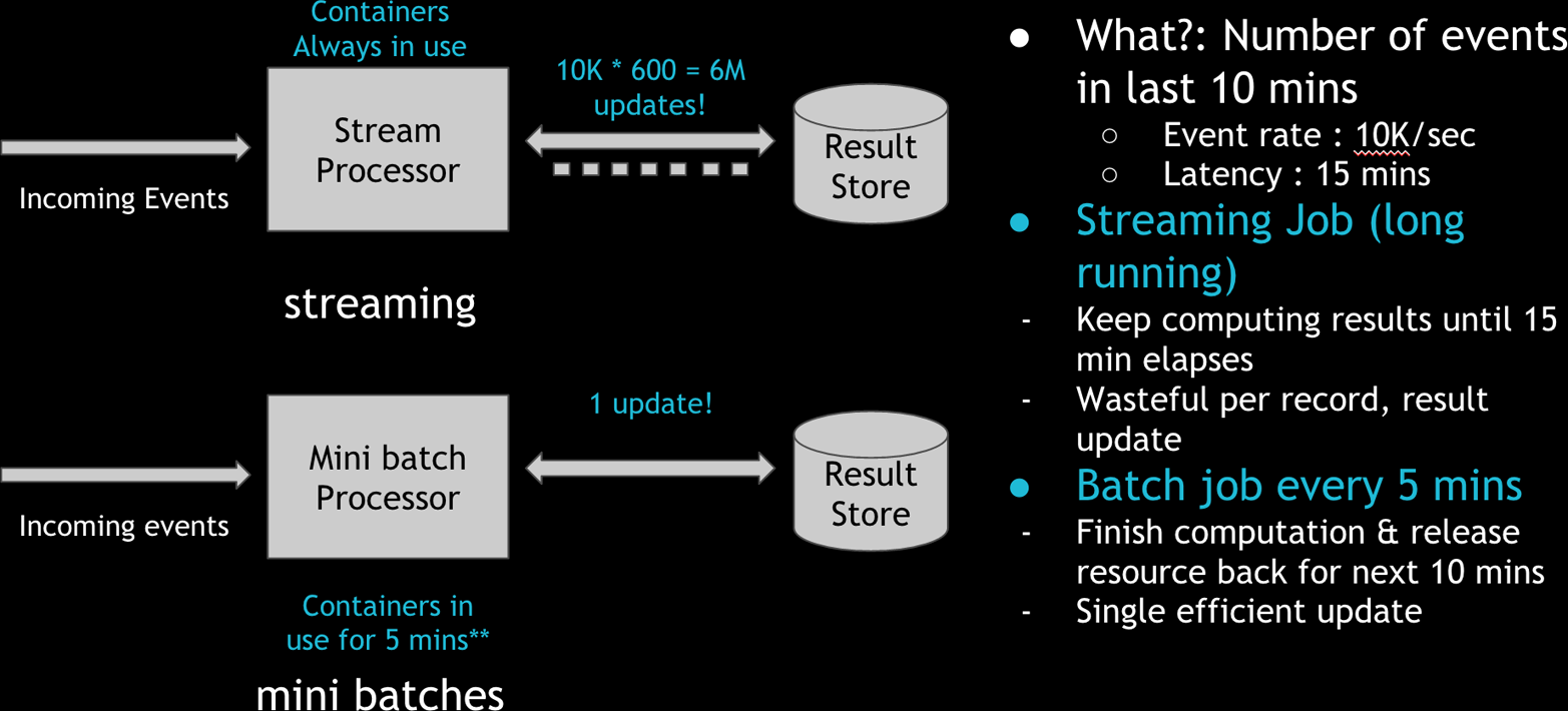
Figure 3-7. Comparison of processing via stream processing engines versus incremental “mini” batch jobs. Credit: Vinoth Chandar.

However, in the near-real-time context, these decisions may not be the best ones. To achieve the same effect, you can use short-lived containers and improve the overall resource utilization. In Figure 3-7, the stream processor performs six million updates over 15 minutes to the result store. But in the incremental processing model, we perform in-memory merge once and only one update to the result store, while using the containers for only five minutes. The incremental processing model is three times more CPU-efficient, and several magnitudes more efficient on updating of the result store. Basically, instead of waiting for work and eating up CPU and memory, the processing wakes up often enough to finish up pending work, grabbing resources on demand.

Built on top of existing SQL engines

Over time, a slew of SQL engines have evolved in the Hadoop/big data space (e.g., Hive, Presto, SparkSQL) that provide better expressibility for complex questions against large volumes of data. These systems have been deployed at massive scale and have hardened over time in terms of query planning, execution, and so forth. On the other hand, SQL on stream processing is still in early stages. By performing incremental processing using existing, much more mature SQL engines in the Hadoop ecosystem, we can leverage the solid foundations that have gone into building them.

For example, joins are very tricky in stream processing, in terms of aligning the streams across windows. In the incremental processing model, the problem naturally becomes simpler due to relatively longer windows, allowing more room for the streams to align across a processing window. On the other hand, if correctness is more important, SQL provides an easier way to expand the join window selectively and reprocess.

Another important advancement in such SQL engines is the support for columnar file formats like ORC/Parquet, which have significant advantages for analytical workloads. For example, joining two Kafka topics with Avro records would be much more expensive than joining two Hive/Spark tables backed by ORC/Parquet file formats. This is because with Avro records, you would end up deserializing the entire record, whereas columnar file formats only read the columns in the record that are needed by the query. For example, if we are simply projecting out 10 fields out of a total 1,000 in a Kafka Avro encoded event, we still end up paying the CPU and IO cost for all fields. Columnar file formats can typically be smart about pushing the projection down to the storage layer (Figure 3-8).

Figure 3-8. Comparison of CPU/IO cost of projecting 10 fields out of 1,000 total, as Kafka events versus columnar files on HDFS. Credit: Vinoth Chandar.

Fewer moving parts

The famed Lambda architecture that is broadly implemented today has two components: speed and batch layers, usually managed by two separate implementations (from code to infrastructure). For example, Storm is a popular choice for the speed layer, and MapReduce could serve as the batch layer. In practice, people often rely on the speed layer to provide fresher (and potentially inaccurate) results, whereas the batch layer corrects the results of the speed layer at a later time, once the data is deemed complete. With incremental processing, we have an opportunity to implement the Lambda architecture in a unified way at the code level as well as the infrastructure level.

The idea illustrated in Figure 3-9 is fairly simple. You can use SQL, as discussed, or the same batch-processing framework as Spark to implement your processing logic uniformly. The resulting table gets incrementally built by way of executing the SQL on the “new data,” just like stream processing, to produce a “fast” view of the results. The same SQL can be run periodically on all of the data to correct any inaccuracies (remember, joins are tricky!) to produce a more “complete” view of the results. In both cases, we will be using the same Hadoop infrastructure for executing computations, which can bring down overall operational cost and complexity.

Figure 3-9. Computation of a result table, backed by a fast view via incremental processing and a more complete view via traditional batch processing. Credit: Vinoth Chandar.

Trade-off: completeness versus latency

In computing, as we traverse the line between stream processing, incremental processing, and batch processing, we are faced with the same fundamental trade-off. Some applications need all the data and produce more complete/accurate results, whereas some just need data at lower latency to produce acceptable results. Let’s look at a few examples.

Figure 3-10 depicts a few sample applications, placing them according to their tolerance for latency and (in)completeness. Business dashboards can display metrics at different granularities because they often have the flexibility to show more incomplete data at lower latencies for recent times while over time getting complete (which also made them the marquee use case for Lambda architecture). For data science/machine-learning use cases, the process of extracting the features from the incoming data typically happens at lower latencies, and the model training itself happens at a higher latency with more complete data. Detecting fraud, on the one hand, requires low-latency processing on the data available thus far. An experimentation platform, on the other hand, needs a fair amount of data, at relatively lower latencies, to keep results of experiments up to date.

Figure 3-10. Figure showing different Hadoop applications and their tolerance for latency and completeness. Credit: Vinoth Chandar.

The most common cause for lack of completeness is late-arriving data (as explained in detail in this Google Cloud Dataflow deck). In the wild, late data can manifest in infrastructure-level issues, such as data center connectivity flaking out for 15 minutes, or user-level issues, such as a mobile app sending late events due to spotty connectivity during a flight. At Uber, we face very similar challenges, as we presented at Strata + Hadoop World in March 2016.

To effectively support such a diverse set of applications, the programming model needs to treat late-arrival data as a first-class citizen. However, Hadoop processing has typically been batch-oriented on “complete” data (e.g., partitions in Hive), with the responsibility of ensuring completeness also resting solely with the data producer. This is simply too much responsibility for individual producers to take on in today’s complex data ecosystems. Most producers end up using stream processing on a storage system like Kafka to achieve lower latencies while relying on Hadoop storage for more “complete” (re)processing. We will expand on this in the next section.

Lack of primitives for incremental processing

As detailed in this article on stream processing, the notions of event time versus arrival time and handling of late data are important aspects of computing with lower latencies. Late data forces recomputation of the time windows (typically, Hive partitions in Hadoop), over which results might have been computed already and even communicated to the end user. Typically, such recomputations in the stream processing world happen incrementally at the record/event level by use of scalable key-value stores, which are optimized for point lookups and updates. However, in Hadoop, recomputing typically just means rewriting the entire (immutable) Hive partition (or a folder inside HDFS for simplicity) and recomputing all jobs that consumed that Hive partition.

Both of these operations are expensive in terms of latency as well as resource utilization. This cost typically cascades across the entire data flow inside Hadoop, ultimately adding hours of latency at the end. Thus, incremental processing needs to make these two operations much faster so that we can efficiently incorporate changes into existing Hive partitions as well as provide a way for the downstream consumer of the table to obtain only the new changes.

Effectively supporting incremental processing boils down to the following primitives:

Upserts

Conceptually, rewriting the entire partition can be viewed as a highly inefficient upsert operation, which ends up writing way more than the amount of incoming changes. Thus, first-class support for (batch) upserts becomes an important tool to possess. In fact, recent trends like Kudu and Hive Transactions do point in this direction. Google’s “Mesa” paper also talks about several techniques that can be applied in the context of ingesting quickly.

Incremental consumption

Although upserts can solve the problem of publishing new data to a partition quickly, downstream consumers do not know what data has changed since a point in the past. Typically, consumers learn this by scanning the entire partition/table and recomputing everything, which can take a lot of time and resources. Thus, we also need a mechanism to more efficiently obtain the records that have changed since the last time the partition was consumed.

With the two primitives above, you can support a lot of common use cases by upserting one data set and then incrementally consuming from it to build another data set incrementally. Projections are the most simple to understand, as depicted in Figure 3-11.

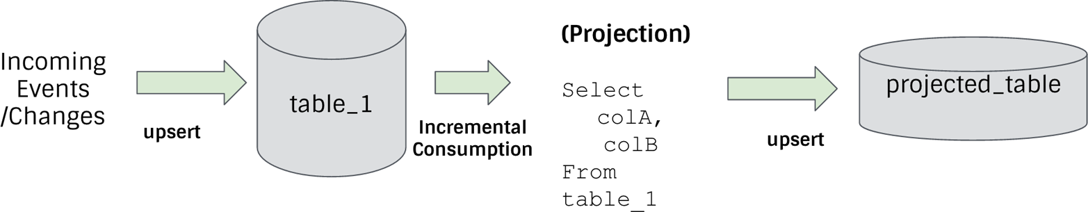
Figure 3-11. Simple example of building of table_1 by upserting new changes, and building a simple projected_table via incremental consumption. Credit: Vinoth Chandar.

Borrowing terminology from Spark Streaming, we can perform simple projections and stream-data set joins much more efficiently at lower latency. Even stream-stream joins can be computed incrementally, with some extra logic to align windows (Figure 3-12).

This is actually one of the rare scenarios where we could save money with hardware while also cutting down the latencies dramatically.

Figure 3-12. More complex example that joins a fact table against multiple dimension tables, to produce a joined table. Credit: Vinoth Chandar.

Shift in mindset

The final challenge is not strictly technical. Organizational dynamics play a central role in which technologies are chosen for different use cases. In many organizations, teams pick templated solutions that are prevalent in the industry, and teams get used to operating these systems in a certain way. For example, typical warehousing latency needs are on the order of hours. Thus, even though the underlying technology could solve a good chunk of use cases at lower latencies, a lot of effort needs to be put into minimizing downtimes or avoiding service disruptions during maintenance. If you are building toward lower latency SLAs, these operational characteristics are essential. On the one hand, teams that solve low-latency problems are extremely good at operating those systems with strict SLAs, and invariably the organization ends up creating silos for batch and stream processing, which impedes realization of the aforementioned benefits to incremental processing on a system like Hadoop.

This is in no way an attempt to generalize the challenges of organizational dynamics, but is merely my own observation as someone who has spanned the online services powering LinkedIn as well as the data ecosystem powering Uber.