CHAPTER 11
Understand Text Analytics
“Seek success but prepare for vegetables.”
InspireBot™, an AI bot “dedicated to generating unlimited amounts of unique inspirational quotes.”1
The last several chapters have dealt with data as we commonly understand it. For most of us, datasets are tables with rows and columns. That's structured data. In reality, though, most of the data you interact with every day is unstructured. It's in the text you read. It's in the words and sentences of emails, news articles, social media posts, Amazon product reviews, Wikipedia articles, and this book in your hands.
That unstructured textual data is ripe for analysis, but it has to be treated a bit differently. That's what this chapter is about.
EXPECTATIONS OF TEXT ANALYTICS
Before we dive in, we want to set your expectations. Text analytics has received a lot of attention and focus over the years. One example is sentiment analysis—that is the ability to identify the positive or negative emotions behind a social media post, a comment, or a complaint. But as you'll see, text analytics is not such an easy thing to do. By the end of this chapter, you'll have a sense of why some companies can succeed in its use while others will have their work ahead of them.
Many people have preconceived notions about what's possible with computers and human language, undoubtedly influenced by the tremendous success of IBM's Watson computer on the quiz show Jeopardy! in 20112 and the more recent advancements in speech-recognition systems (think Amazon's Alexa, Apple's Siri, and Google's Assistant). Translations systems, like Google Translate, have achieved near human-level performance by leveraging machine learning (specifically, supervised learning). These applications are held up, rightfully so, as some of the most towering achievements in computer science, linguistics, and machine learning.
Which is why, in our estimation, businesses have exceedingly high expectations when they start analyzing their own text data: customer comments, survey results, medical records—whatever text is stored in your databases. If world travelers can translate their native tongue into one of over 100 languages in a split second, surely it's possible to sift through thousands of your business's customer comments and identify the most pressing issues to your company. Right?
Well, maybe.
Text analytic technologies, while able to solve huge, difficult problems like voice-to-text and speech translation often fail at tasks that seem much easier. And in our experience, when companies analyze their own text data, there's often disappointment and frustration with the results. Put simply, text analytics is harder than you might realize. So, as a Data Head, you'll want to set expectations accordingly.
Our goal in this chapter, then, is to teach you some of the basics of text analytics,3 which is extracting useful insights from raw text. To be clear, we can only scratch the surface of this burgeoning field, but we hope to provide you with enough information to give you a feel of the possibilities and challenges of text analytics. As new developments come about in this space, you'll have the tools to understand what will help and what won't. And, as with any topic, the more you learn, the more you'll naturally build awareness to what's possible but also come away with some warranted Data Head skepticism.
In the sections that follow, we'll talk about how to gain structure from your unstructured text data, what kind of analysis you can do on it, and then we'll revisit why Big Tech can make seemingly science fiction-like progress with their text data while the rest of us might struggle.
HOW TEXT BECOMES NUMBERS
When humans read text, we see mood, sarcasm, innuendo, nuance, and meaning. Sometimes that feeling is even unexplainable: a poem is evocative of a memory; a joke makes you laugh.
So it's likely not a surprise that a computer does not understand meaning the way a human does. Computers can only “see” and “read” numbers. The mass of unstructured text data must first be converted to numbers and the structured datasets you're familiar with in order to be analyzed. This process—converting unstructured and potentially messy text with misspellings, slang, emojis, or acronyms into a tidy, structured dataset with rows and columns—can be a subjective and time-consuming process for you and your data workers. There are several ways to do it, and we'll cover three.
A Big Bag of Words
The most basic approach to convert text into numbers is by creating a “bag of words” model. In a bag of words, a sentence of text is jumbled together into a “bag” where word order and grammar are ignored. What you read as: “This sentence is a big bag of words” is converted into a set, called a document, where each word is an identifier, and the count of the word is a feature. Order does not matter, so we'll sort the bag alphabetically by identifier:
{a: 1, bag: 1, big: 1, is: 1, of: 1, sentence: 1, this: 1, words: 1}.
Each identifier is referred to as a token. The entire set of tokens from all documents is called a dictionary.
Of course, your text data will contain more than one document, so this bag of words can get exceedingly large. Every unique word and spelling would become a new token. Here's how this would look as a table, where each row contains a sentence (or customer comment, product review, etc.).
For the raw text:
- This sentence is a big bag of words.
- This is a big bag of groceries.
- Your sentence is two years.
The bag-of-words representation would look like that in Table 11.1, where the data points represent the count of each word in the sentence.
TABLE 11.1 Converting Text to Numbers as a Bag of Words . The numbers represent how many times each word (token) appears in the corresponding sentence (document).
| Original Text | a | bag | big | groceries | is | of | sentence | this | two | words | years | your |
| This sentence is a big bag of words. | 1 | 1 | 1 | 0 | 1 | 1 | 1 | 1 | 0 | 1 | 0 | 0 |
| This is a big bag of groceries. | 1 | 1 | 1 | 1 | 1 | 1 | 0 | 1 | 0 | 0 | 0 | 0 |
| Your sentence is two years. | 0 | 0 | 0 | 0 | 1 | 0 | 1 | 0 | 1 | 0 | 1 | 1 |
Looking at Table 11.1, called a document-term matrix (one document per row, one term per column), you'll notice how easy it would be to perform some basic text analytics: calculating summary statistics of each word (“is” is the most popular word) and finding out which sentence contains the most tokens (first sentence). While not interesting in this example, this is how basic summary statistics of documents can be calculated.
We suspect you've also noticed some drawbacks in Table 11.1 (and hopefully word clouds!). As more documents are added, the number of columns in the table would become exceedingly wide because you'd have to add a new column for each new token. The table would also become very sparse—full of zeros—because each individual sentence would only contain a handful of words from the dictionary.
To combat this, it's standard practice to remove common filler words—like the, of, a, is, an, this, etc.—that don't add meaning or differentiation between sentences. These are called stop words. It's also common to remove punctuation and numbers, convert everything to lowercase, and stem words (cut off their endings) to map words like grocery and groceries to the same stem groceri, or reading, read, reads to read. A more advanced counterpart to stemming is called lemmatization, which would map words good, better, best to the root word good. In that sense, lemmatization is “smarter” than stemming, but it takes longer to process.
Little adjustments like this can drastically reduce the size of the dictionary and make analysis easier. Figure 11.2 shows what this process would look like for one sentence.
It should come as no surprise then, after seeing this approach in Figure 11.2, why analyzing text is hard. The process to convert text into numbers has filtered out emotion, context, and word order. If you suspect this would impact the results of any subsequent analysis, you'd be right. And we were lucky here—there aren't any misspellings, which are an added challenge for data workers.
Using the bag-of-words approach, which is available in free software and the first approach data workers learn in text analytics courses, would provide the same numerical encoding for the following two sentences, despite the obvious difference in meaning:
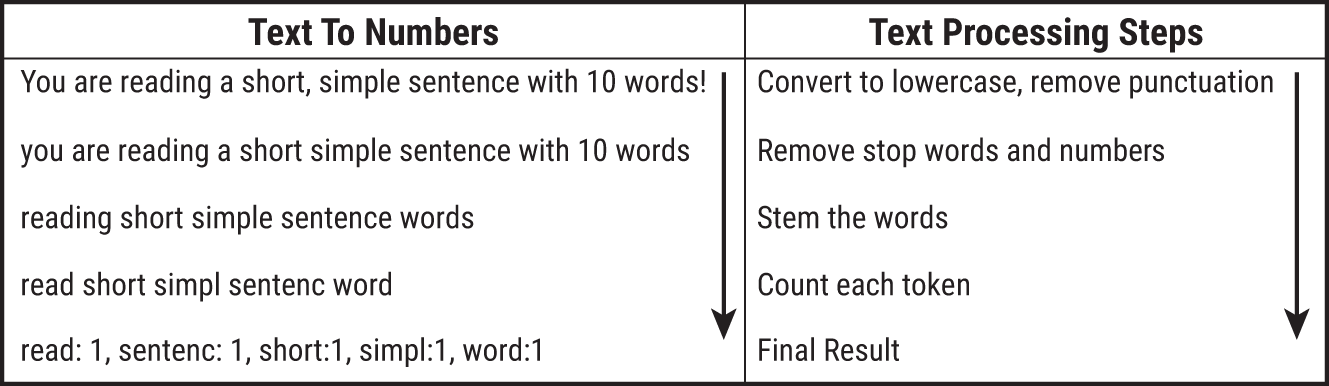
FIGURE 11.2 Processing text down to a bag of words
- Jordan loves hotdogs but hates hamburgers.5
- Jordan hates hotdogs but loves hamburgers.
Humans know the difference between those two sentences. A bag-of-words approach does not. But make no mistake. Despite its simplistic approach, a bag of words can be helpful when summarizing very disparate topics, which we'll highlight in later sections.
N-Grams
It's easy to see where the bag-of-words approach let us down in the example about Jordan and his hotdogs. The two-word phrase “loves hotdogs” is the opposite of “hates hotdogs,” but bag-of-words throws context and word order aside. N-grams can help. An N-gram is a sequence of N consecutive words, so the 2-grams (formally called bigrams) for the sentence “Jordan loves hotdogs but hates hamburgers” would be: {but hates: 1, hates hamburgers: 1, hotdogs but: 1, Jordan loves: 1, loves hotdogs: 1}
It's an extension of bag-of-words but adds the context we need to differentiate phrases with identical words in different arrangements. It's common to add the bigram tokens to the bag-of-words, which further increases the size and sparseness of the document-term matrix. From a practical matter, this means you need to store a large (wide) table with relatively little information inside. We added some bigrams to Table 11.1 to create Table 11.2.
There are some debates whether to filter out bigrams with stop words, as context can be lost. The words “my” and “your” are considered stop words in some software, but the meaning behind the bigram phrases “my preference” and “your preference” is gone if stop words are removed. This is another decision your data workers must make when analyzing text data. (Can you start to sense why text analytics is challenging?)
But once prepared, simple counts can be helpful to summarize text. Websites like Tripadvisor.com take advantage of these approaches and give users the ability to quickly search reviews for frequently mentioned words or phrases. You might see, for example, suggested searches like “baked potato” or “prepared perfectly” as commonly mentioned bigrams at your local steakhouse.
TABLE 11.2 Extending the Bag-of-Words Table with Bigrams. The resulting document-term matrix gets very wide.
| a | bag | big | groceries | is | of | sentence | this | two | words | years | your | a big | big bag | is a | sentence is | this sentence | of groceries | this is | bag of | … |
|---|---|---|---|---|---|---|---|---|---|---|---|---|---|---|---|---|---|---|---|---|
| 1 | 1 | 1 | 0 | 1 | 1 | 1 | 1 | 0 | 1 | 0 | 0 | 1 | 1 | 1 | 1 | 1 | 0 | 0 | 1 | … |
| 1 | 1 | 1 | 1 | 1 | 1 | 0 | 1 | 0 | 0 | 0 | 0 | 1 | 1 | 1 | 0 | 0 | 1 | 1 | 1 | … |
| 0 | 0 | 0 | 0 | 1 | 0 | 1 | 0 | 1 | 0 | 1 | 1 | 0 | 0 | 0 | 1 | 0 | 0 | 0 | 0 | … |
Word Embeddings
With bag-of-words and N-grams, it's possible to tell similarity between documents: if multiple documents contain similar sets of words or N-grams, you can reasonably assume the sentences are related (within reason, of course. Don't forget about Jordan's love/hate relationship with hotdogs). The rows in the document-term matrix would be numerically similar.
But how could someone go about discovering, numerically, which words in a dictionary—not documents, but words—are related?
In 2013, Google analyzed billions of word pairs (two words within close proximity of each other within a sentence) in its enormous database of Google News articles.6 By analyzing how often word pairs appeared—for example, (delicious, beef) and (delicious, pork) appeared more than (delicious, cow) and (delicious, pig)—they were able to generate what are called word embeddings, which are numeric representations of words as a list of numbers (aka vectors). If beef and pork appear often with the word delicious, the math would represent each word as being similar in an element of the vector associated with things described as delicious, or what we humans would simply call food.
To explain how it works, we'll use a tiny set of word pairs (Google used billions). Suppose we scan a local newspaper article and find the following pairs of words: (delicious, beef), (delicious, salad), (feed, cow), (beef, cow), (pig, pork), (pork, salad), (salad, beef), (eat, pork), (cow, farm), etc. (Imagine several more pairs along this line of thinking.) Every word goes into the dictionary: {beef, cow, delicious, farm, feed, pig, pork, salad}.7
The word cow, for example, can be represented as a vector the length of the preceding dictionary—one component per word with a 1 in the location of cow and zero otherwise: (0, 1, 0, 0, 0, 0, 0, 0). This is an input into a supervised learning algorithm that is mapped to its associated output vector (also the length of the dictionary). In it are the probabilities that the other words in the dictionary appeared near the input word. So for input cow, the associated output might be (0.3, 0, 0, 0.5, 0.1, 0.1, 0, 0), to show cow was paired with beef 30% of the time, farm 50% of the time, and feed & pig 10% of the time.
As is the goal with every supervised learning problem, the model tries to map the inputs (word vectors) as close as possible to the outputs (vectors with probabilities). But here's the twist. We don't care about the model itself; we care about a piece of math generated from the model: a table of numbers that shows how each word in the dictionary relates to every other word. These are the word embeddings. Think of them as a numeric representation of a word that encodes its “meaning.” Table 11.3 shows some of the words in our dictionary, along with their word embeddings across the rows. Cow, for example, is written as a three-dimensional vector (1.0, 0.1, 1.0). Before, it was written as the longer, sparser vector (0, 1, 0, 0, 0, 0, 0, 0).
What's fascinating about word embeddings is that the dimensions (hopefully) contain meaning behind the words, similar in a way to how the reduced dimensions in PCA captured themes of features.
TABLE 11.3 Representing Words as Vectors with Word Embeddings
| Word | Dimension 1 | Dimension 2 | Dimension 3 |
|---|---|---|---|
| Cow | 1.0 | 0.1 | 1.0 |
| Beef | 0.1 | 1.0 | 0.9 |
| Pig | 1.0 | 0.1 | 0.0 |
| Pork | 0.1 | 1.0 | 0.0 |
| Salad | 0.0 | 1.0 | 0.0 |
Look down Dimension 1 in Table 11.3. Can you spot a pattern? Whatever Dimension 1 means, Cow and Pig have a lot of it, and Salad has none of it. We might choose to call this Dimension Animal. Dimension 2, we can call Food because Beef, Pork, and Salad scored high, and Dimension 3 Bovine because words associated with cows stood out. With this structure, it's now possible to see similarities in how words are used. It's even possible (if a bit weird) to show simple equations between words.
As an exercise, convince yourself (using Table 11.3) that Beef – Cow + Pig ≈ Pork.8
This technique is called Word2vec9 (word to vector) and the word embeddings Google generated for us are freely available to download.10 Of course, don't expect every relationship to be perfect. There's variation in all things, as you're astutely aware of by now, and it's certainly present in text. Non-food items can be described as delicious, like delicious irony. There's orange the color and orange the juice, and a plethora of homonyms in our language to complicate things.
Word embeddings, with their numeric structure that enables calculation, have applications in search engines and recommendation systems, but the word embeddings generated from Google News text might not be specific to your problem set. For example, brand names like Tide® (laundry detergent) and Goldfish® (crackers) may be semantically similar to the words “ocean” and “pet,” respectively, in a system like Word2vec, but for a grocery store, those items would be semantically more similar to competing brands like Gain® detergent and Barnum's Animals® crackers.
It is possible to run Word2vec on your text data and generate your own word embeddings. This would help you glean topics and concepts you might otherwise not even consider in your data. However, getting enough data to be meaningful is an issue. Not every company will have access to as much data as Google. You simply may not have enough text data to find meaningful word embeddings.
TOPIC MODELING
Once we have our text into a meaningful dataset, we're ready to start some analysis. And, there's a satisfying payoff to this investment of converting unstructured text data into a structured dataset with rows and columns of numbers. That's because we can use those analysis methods you've been learning about throughout this book (with some tweaks). Let's talk about those analysis methods in the next few sections.
In Chapter 8, you learned about unsupervised learning—finding natural patterns in the rows and columns of a dataset. Unleashing a clustering algorithm like k-means on a document-term matrix, like in Tables 11.1 and 11.2, would produce a set of k distinct groups of text that are similar in some way. This could prove to be helpful in some cases. But applying k-means clustering to text data is quite rigid. Consider, for instance, these three sentences:
- The Department of Defense should outline an official policy for outer space.
- The Treaty on the Non-Proliferation of Nuclear Weapons is important for national defense
- The United States space program recently sent two astronauts into space.
In our eyes, there are two general topics being discussed here: national defense and space. The first sentence discusses both topics, while the second and third touch on one. (If you disagree, and you're certainly allowed to, then you are realizing a central challenge of clustering text together—there's not always a clean separation of topics. And with text, unlike a row of numbers, everyone can quickly form an opinion.)
Topic modeling11 is similar in spirit to k-means in the sense that it's an unsupervised learning algorithm that attempts to group similar observations together, but it relaxes the notion that each document should be explicitly assigned to one cluster. Instead, it provides probabilities to show how one document might span across several topics. Sentence 1, for example, might score 60% for national defense and 40% for space.
A new example will help. In Figure 11.3, you see a visual representation of a document-term matrix flipped on its side.12 Along the left, you see the terms that appear in the 20 documents along the top, denoted d0 though d19. Each cell represents the frequency of a word in the document, with darker cells indicating a higher frequency. But the terms and documents have been arranged, via topic modeling, to reveal the results of the topic model.
Study the image, and you'll spot which words appear frequently in documents together forming possible topics, as well as documents that contain several terms that are woven across multiple topics (look at d13 specifically, the third column from the right). Be advised, though—like all unsupervised learning methods, there's no guarantee of accurate results.

FIGURE 11.3 Clustering documents and terms together with topic modeling. Can you spot the five main topics in the image? What would you name them?
As a practical matter, topic modeling works best when there are disparate topics within your set of documents. That may seem obvious, but we've seen instances where topic modeling has been applied on subsets of text that have been filtered down to a specific topic of interest prior to the analysis. This would be like taking a group of news articles, searching for only those that contain “basketball” and “LeBron James” and then expecting topic modeling to break out the remaining articles into something meaningful. You'll be disappointed with the results. By filtering the text, you've effectively defined one topic for the articles that remain. Keep this nuance in mind, continue to argue with your data, and manage expectations appropriately.
TEXT CLASSIFICATION
In this section, we'll switch from unsupervised learning to supervised learning on a document-term matrix (provided a known target exists to learn from). With text, we're usually trying to predict a categorical variable, so this falls under the classification models you learned last chapter, as opposed to regression models that predict numbers. One of the most well-known text classification success stories is the spam filter in your email, where the input is the text of an email, and the output is a binary flag of “spam” or “not spam.”13 A multiclass classification application of text analytics is the automatic assignment of online news articles to the news categories: Local, Politics, World, Sports, Entertainment, etc.
Let's look at one (oversimplified) case to give you an idea how text classification works using bag-of-words. Table 11.4 shows five different email subject lines, broken out into tokens, and a label indicating if the email is spam or not. (As an aside, let's not discount the effort companies take to collect data like this. There's a reason your email provider asks you if your email is spam or not. You are providing the training data for machine learning algorithms!)
How might we use an algorithm to learn from the data in Table 11.4 to make predictions about new, unseen email subject lines?
TABLE 11.4 A Basic Spam Classifier Example
| Email Subject | advice | bald | birthday | debt | free | help | mom | party | relief | stock | viagra | Spam? |
|---|---|---|---|---|---|---|---|---|---|---|---|---|
| Advice for Mom's birthday party | 1 | 0 | 1 | 0 | 0 | 0 | 1 | 1 | 0 | 0 | 0 | 0 |
| Free Viagra! | 0 | 0 | 0 | 0 | 1 | 0 | 0 | 0 | 0 | 0 | 1 | 1 |
| Free Stock Advice | 1 | 0 | 0 | 0 | 1 | 0 | 0 | 0 | 0 | 1 | 0 | 1 |
| Free Debt Relief Advice | 1 | 0 | 0 | 1 | 1 | 0 | 0 | 0 | 1 | 0 | 0 | 1 |
| Balding? We can help! | 0 | 1 | 0 | 0 | 0 | 1 | 0 | 0 | 0 | 0 | 0 | 1 |
Perhaps you thought of logistic regression, which is useful to predict binary outcomes. Unfortunately, logistic regression will not work here. Why not? The math behind logistic regression breaks down because there are too many words and not enough examples to learn from. There are more columns than rows in Table 11.4, and logistic regression doesn't like that.14
Naïve Bayes
The popular method to apply in this situation is a classification algorithm called Naïve Bayes (named after the very same Bayes we mentioned in Chapter 6). The intuition behind it is straightforward: are the words in the email subject line more likely to appear in a spam email or a non-spam email? You probably perform a similar process to this when you read your inbox: the word “free,” based on your experience, is typically a spammy word. As is “money,” “Viagra,” or “rich.” If most words are spammy, the email is probably spam. Easy.
Said another way, you're trying to calculate the probability an email is spam, given the words in the subject line, (w1, w2 , w3 , …). If this probability is greater than the probability it's not spam, mark the email as spam. In probability notation, these competing probabilities are written as:
- Probability an email is spam = P(spam | w1, w2 , w3 , ...)
- Probability an email is not spam = P(not spam | w1, w2 , w3 , …)
Before moving on, let's take stock of the data available to us in Table 11.4. We have the probability that each word occurs in spam (and not spam) emails. “Free” occurred in three out of the four spam emails, so the probability of seeing “free,” given the email is spam, is P(free | spam) = 0.75. Similar calculations would show: P(debt | spam) = 0.25, P(mom | not spam) = 1, and so on.
What does that give us? We want to know the probability an email is spam given the words, but what we have is the probability of seeing a word, given it's spam. These two probabilities are not the same, but they are linked through Bayes’ Theorem (from Chapter 6). Recall the central idea behind Bayes’ is to swap the conditional probabilities. Thus, instead of working with P(spam | w1, w2 , w3 , ...), we can use P(w1, w2 , w3 , … | spam). Through some additional math (which we're skipping for brevity15), the decision to classify a new email as spam comes down to figuring out which value is higher:
- Spam score = P(spam) × P(w1 | spam) × P(w2 | spam) × P(w3 | spam)
- Not Spam score = P(not spam) × P(w1 | not spam) × P(w2 | not spam) × P(w3 | not spam)
All of this information is available in Table 11.4. The probabilities P(spam) and P(not spam) represent the proportion of spam and not spam in the training data—80% and 20%, respectively. In other words, if you had to take a guess without looking at the subject line, you'd guess “spam” because that's the majority class in the training data.
In order to get to the preceding formulas, the Naïve Bayes approach committed what is usually an egregious error in probability—assuming independence between events. The probability of “free” and “Viagra” appearing in a spam email together, denoted P(free, viagra | spam) depends on how often both words appear in the same email, but this makes the computation much more difficult. The “naïve” part of Naïve Bayes is to assume every probability is independent: P(free, viagra | spam) = P(free | spam) × P(viagra | spam).
But there's a slight problem. New and rare words require some adjustments to calculations to avoid multiplying the probabilities by zero. In the tiny dataset in Table 11.4, the word “get” doesn't appear at all, and the words debt, stock, and advice have only shown up in spam. These quirks would make both the spam and not spam scores equal to zero. To fix this, let's pretend we've seen each word at least once by adding 1 to the frequency of each word. We'll also add 2 to the frequency of the spam (and not spam) to prevent values from reaching 1.16
Now we can calculate:
- Spam Score:
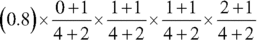 = 0.0074
 - Not Spam Score:
 = 0.0049
The top number is larger, so we'd predict spam for the email: “Get out of debt with our stock advice!”
Sentiment Analysis
Sentiment analysis is a popular text classification application on social media data. If you search Google for “sentiment analysis of Twitter data,” you might be surprised by the number of results; it seems everyone is doing it. The underlying idea is like the spam/not spam example earlier: are the words in a social media post (or product review, or survey) more likely to be “positive” or “negative.” What you do with this information depends on your business cases, but there is an important callout to mention with sentiment analysis: do not extrapolate beyond the context of the training data and expect meaningful results.
What do we mean? Many “sentiment analysis” classifiers learn from freely available data online. A popular dataset for students is a large collection of movie reviewers from the Internet Movie Database (IMDb.com). This collection of data, and any model you build on it, would be relevant to movie reviews only. Sure, it would associate words like “great” and “awesome” with positive sentiment, but don't expect it to perform well if you have a unique business case with its own vernacular.
PRACTICAL CONSIDERATIONS WHEN WORKING WITH TEXT
Now that you're familiar with a handful of tools in the text analytics toolbox, we're going to take a step back in this section and talk about text analytics at a high level.
When working with text, you have the luxury of reading the data. If topic modeling suggests certain sentences belong in topics, review the results for a gut check. If someone builds a text classification model, ask to see the results: the good, the bad, and the ugly.
From experience, a successful text analytics project is fun to present to stakeholders because the audience can read the data and participate in conversations about the results—it's not a series of numbers, but something they can read, understand, and pass judgment of immediately. But presenters are tempted to show the exciting examples and the easy wins, rather than the clear misses. Data Heads, if presenting text analytic results, should be transparent with outcomes. Likewise, if you are consuming results, request to see examples where the algorithms went wrong. Trust us, they exist.
Which brings us back to a comment we made early in the chapter: when companies analyze their own text data, there's often disappointment and frustration with the results. This wasn't to turn you away from text—far from it. By being transparent with the shortcomings, we hope we can prevent a possible backlash where you or your company starts analyzing text, realizes it's trickier than anticipated, and angrily dismisses it entirely or ignores its lack of usefulness and goes full steam ahead with a weak analysis.
By now, you've developed enough skepticism in the earlier sections to realize where hiccups can emerge. But some big tech companies have seemed to rise above those challenges and have emerged as leaders in text analytics and Natural Language Processing (NLP), which deals with all aspects of language, including audio (as opposed to just written text).
Big Tech Has the Upper Hand
Here's what big tech companies like Facebook, Apple, Amazon, Google, and Microsoft have that many other companies don't have: an abundance of text and voice data (an abundance of labeled data that can be used to train supervised learning models); powerful computers; dedicated (and world-class) research teams; and money.
With these resources, they've made remarkable progress not only with text, but also with audio. In recent years, there has been noticeable improvements to the areas of
- Speech-to-Text: Voice-activated assistants and voice-to-text on smartphones are more accurate.
- Text-to-Speech: Computers’ read-aloud voices sound more human-like.
- Text-to-Text: Translating one language to another is instantaneous with good accuracy.
- Chatbots: The automated chat windows that pop up on every website now with: “How may I help you?” are (somewhat) more helpful.
- Generating Human-Readable Text: The language model known as GPT-317 from OpenAI is a language model that can generate human-like text (you might think a human wrote it), answer questions, and generate computer code on demand. And it is, as of this writing, the most advanced model of its kind. Estimates put the cost of training the model (not paying the researchers, just running the computers) at $4.6 million.18
Add to that the access to data and an expert research team, and you get the idea how NLP is often a case of the haves vs. the have nots. Most companies, to be blunt, aren't there (yet?). Even though the algorithms are open source, the massive collection of data and access to supercomputers is not. Big tech clearly has the advantage.
The other thing to consider, when establishing expectations, is how many of the applications from big tech are universal to millions of people; think of them as general tasks common to all sects of society. Amazon Alexa is designed to work for everyone, including children. And when translating text, there are rigid rules built into the training data. The word party in English is the word fiesta in Spanish. Our point is this: everyone who uses these systems is expecting it to work in the same way.
Contrast this to a business-specific text classification task. For example, the sentiment of the sentence “Samsung is better than an iPhone” depends on whether you work for Apple or Samsung. The data you have access to may have its own type of language, unique to only your company. Not only that, but the size of the data will be smaller than what tech companies have available. Consequently, results may not be as clean as you would expect.
Still, we strongly encourage you to avail yourself of all available algorithms including text analytics. Insight is not a matter of big machines, but rather a matter of context and expectation. If you understand the limitations of text analytics before you start, you'll be prepared to run it correctly at your company.
CHAPTER SUMMARY
By going through this chapter, we hope we've convinced you that computers don't understand language as humans do—to a computer, it's all numbers. This alone, in our opinion, is incredibly valuable to know. You're less likely to be swindled the next time you hear marketing rhetoric about how artificial intelligence can solve every text-related business problem you can think of because the process of converting text to numbers removes some of the meaning we as humans would assign to words and sentences. We discussed three methods:
- Bag of words
- N-grams
- Word embeddings
When converted to numbers, you can apply unsupervised learning tasks like topic modeling or supervised learning tasks like text classification. Finally, we described how Big Tech has the upper hand, so set your expectations accordingly based on the amount of data and resources you have.
In the next chapter, we'll continue our analysis of unstructured data to describe neural networks and deep learning.
NOTES
- 1 Generate your own inspiring quotes at
inspirobot.me - 2 There's a great description of Watson's question-answering system in the book: Siegel, E. (2013). Predictive analytics: The power to predict who will click, buy, lie, or die. John Wiley & Sons.
- 3 You might also hear text mining.
- 4 Word cloud generated by wordclouds.com.
- 5 Jordan's favorite food is hotdogs.
- 6 A more in-depth description of Word2vec is presented in Chapter 11 of the outstanding book: Mitchell, M. (2019). Artificial intelligence: A guide for thinking humans. Penguin UK.
- 7 Yes, we are ignoring many pairs of words that would occur, even in the shortest of articles. This alone should convince you of the computational challenge Google had to undertake to do this.
- 8 Beef = (0.1, 1, 0.9), Cow = (1.0, .1, 1.0), Pig = (1.0, 0.1, 0.0). Add/subtract the elements. Beef – Cow + Pig = (0.1, 1, -0.1), which is close to Pork = (0.1, 1.0, 0).
- 9 Mikolov, T., Chen, K., Corrado, G., & Dean, J. (2013). Efficient estimation of word representations in vector space. arXiv preprint arXiv:1301.3781.
- 10 code.google.com/archive/p/word2vec
- 11 Two popular types of topic modeling are Latent Semantic Analysis (LSA) and Latent Dirichlet Allocation (LDA).
- 12 This figure is from en.wikipedia.org/wiki/File:Topic_model_scheme.webm, created by Christoph Carl King and made available on Wikipedia under the Creative Commons Attribution-Share Alike 4.0 International license.
- 13 Drucker, H., Wu, D., & Vapnik, V. N. (1999). Support vector machines for spam categorization. IEEE Transactions on Neural networks, 10(5), 1048−1054 is one of the seminal papers in this area.
- 14 Linear regression also does not work if there are more features than observations in the data. However, there are variants of linear and logistic regression that can handle more features than observations.
- 15 For more details, see the Wikipedia article on “Naïve Bayes spam filtering.”
- 16 This is called a Laplace correction. It helps prevent high variability caused by low counts, something we discussed in Chapter 3.
- 17 Generative Pre-trained Transformer 3
- 18 www.forbes.com/sites/bernardmarr/2020/10/05/what-is-gpt-3-and-why-is-it-revolutionizing-artificial-intelligence/#116e7b04481a