CHAPTER 6
Examine the Probabilities
Many people's notion of probability is so impoverished that it admits [one] of only two values: 50-50 and 99%, tossup or essentially certain.”
—John Allen Paulos, mathematician and author of “Innumeracy: Mathematical Illiteracy and Its Consequences”1
Let's talk about probability—the language of uncertainty—and rekindle the conversation we started in Chapter 3, “Prepare to Think Statistically.” To recap, there's variation in all things; variation creates uncertainty; and probability and statistics are tools to help us manage uncertainty.
Our all-too-brief section on probability ended with a message: be mindful and recognize that your intuition can play tricks on you.
A fair statement, but such topics like probability deserve more than a bumper sticker warning. Complete understanding, if there is such a thing, requires reading massive textbooks, listening to long lectures, and a lifetime of study and debate. Even then, experts disagree on the interpretation and philosophy of probability.2 You might not have the time or desire for that level of discussion (neither do we), so we'll spare you those debates and keep the focus on what you need to know to keep your intuition sharp and be successful in your work.
Our goal in this chapter, then, is to move you beyond a bumper sticker grasp of probability and to teach you some of its language, notation, tools, and traps. By the end of this chapter, you will be able to think and speak about probabilities in the workplace, even if you are not the one calculating the numbers—and you will be able to ask hard questions of probabilities presented to you. Indeed, the willingness to wade into discussions about probability and uncertainty is an important step in your development as a Data Head.
TAKE A GUESS
Here's a thought exercise to get you started.
Your Fortune 500 company was the victim of a cyber-attack, and hackers infected 1% of all laptop computers with a virus. The valiant IT team quickly creates a way to test if a laptop is infected. It's a good, almost perfect test. In fact, the IT team's research shows that if the laptop has the virus, the test will be positive 99% of the time. And if a laptop does not have the virus, the test will come back negative 99% of the time.
The team finally tests your laptop for the virus—the result, positive. The question is, what is the probability your laptop actually has the virus?
Take a moment to think of an answer before moving on.
The correct answer is 50%. (We'll prove it later in the chapter.)
Surprised? Most people are.
The answer isn't intuitive. In fact, you knew probability could play tricks on your mind, and it still did. That's the frustrating thing about probability—every problem is a brainteaser. Don't feel discouraged, however, if you got the wrong answer. The real test is whether you paused to think about how uncertain you were before peeking at the answer. Did you?
Not everyone does. The truth is that most people don't have a grasp of, or respect for, probability. Want proof? People still buy scratch-off lottery tickets, flock to Las Vegas, and buy the extended warranty on their television. They are content being woefully ignorant about probability—especially when decisions are tied to a potential payoff (slot machines) or avoiding perceived future frustration (television warranties). Luckily, this chapter will give you a firm grasp of probability, its rules, and its misconceptions.
Let's get started.
THE RULES OF THE GAME
Probability lets us quantify the likelihood that an event will occur.
Before we introduce the math, it's worth considering that our brains are wired for probabilities, in that we use probabilistic statements all the time in daily life. For any event in your life, you don't know for certain exactly what will happen, but you do know that some outcomes are more likely than others. For example, you might hear around the office:
- “It's highly probable they'll sign the contract!”
- “There's a small chance we'll miss next Monday's deadline.”
- “It's doubtful we'll hit our quarterly goals.”
- “Trevor usually shows up late to meetings.”
- “The weather channel says it's likely to rain today—let's move the company retreat.”
But these everyday probability terms are mushy enough to seem correct, even when they're not. Indeed, two people might have different perceptions of how often a “highly probable” or “likely” event occurs—which means everyday language isn't going to cut it. We need to use numbers, data, and notation to quantify probability statements so that what we say is more than just a gut feeling (even if our gut feelings have a high degree of reliability). Not only that, we need to abide by certain rules and logic in probability.
Notation
Probability, as we said earlier, lets us quantify the likelihood that an event will occur. An event can be any outcome, from basic (flipping heads on a coin) to the complex (“Donald Trump will win the 2016 election”). A child can understand the 50-50 chance of flipping a coin, but the entirety of the polling and forecasting industry struggled to predict the 2016 election, even after analyzing terabytes of data.
We'll focus on the simple cases for this quick lesson.
Probability is measured by a number between 0 and 1, inclusive, with 0 being impossible (rolling a 7 on a six-sided die numbered 1−6) and 1 being certain (rolling a number less than 7 on a six-sided die). It's often expressed as a simple fraction (flipping heads on a coin has probability 1/2), or as a percentage (you have a 25% chance of picking a “spade” from a standard deck of playing cards). Many people use all of these—numbers, fractions, and percentages—interchangeably.
To save space, we use shorthand and call probability P. Descriptions of events are also condensed. For example, “The probability of flipping a fair Coin on Heads equals 1/2” can be shorted to P(C == H) = 1/2. Or, even shorter, P(H) = 1/2. In fact, the entire previous paragraph can be written as described in Table 6.1.
TABLE 6.1 Probabilities Scenarios with Associated Notation
| Scenario | Notation |
|---|---|
| Probability of rolling a 7 on a six-sided die | P(D == 7) = 0 |
| Probability of rolling less than a 7 on a six-sided die | P(D < 7) = 1 |
| Probability of picking a spade from a card deck | P(S) = 0.25 |
The notation P(D < 7) = 1 is expressing a cumulative probability—a range of outcomes. It's saying, “The probability you roll a number less than 7 on a Die is 1.” It's adding P(D == 1) + P(D == 2) + P(D == 3) + P(D == 4) + P(D == 5) + P(D == 6) = 6 × 1/6 = 1 (see Table 6.2). The sum of all possible outcomes must equal one.
TABLE 6.2 Cumulative Probability of a Die Roll Less than 7
| Scenario | Notation | Probability |
|---|---|---|
| You roll a 1 | P(D == 1) | 1 / 6 |
| You roll a 2 | P(D == 2) | 1 / 6 |
| You roll a 3 | P(D == 3) | 1 / 6 |
| You roll a 4 | P(D == 4) | 1 / 6 |
| You roll a 5 | P(D == 5) | 1 / 6 |
| You roll a 6 | P(D == 6) | 1 / 6 |
| You roll a number less than 7 | P(D < 7) | 6 / 6 = 1 = 100% |
Conditional Probability and Independent Events
When the probability of an event depends on some other event, it's called a conditional probability and uses notation called a vertical bar, |, read as “given.” A few examples will make this clearer:
- The probability Alex is late to work is 5%. P(A) = 5%.
- The probability Alex is late to work given he has a flat tire is 100%. P(A | F) = 100%.
- The probability Alex is late to work given there's a traffic jam on Interstate 75 is 50%. P(A | T) = 50%.
As you can see, the probability of an event occurring depends heavily on the event, or events, preceding it.
When the probability of an event does not depend on some other event, the two events are independent. For example, the conditional probability of drawing a spade given a coin flipped heads, P(S | H) is the same as the probability of drawing a spade by itself, P(S). In short, P(S | H) = P(S) and, for good measure, P(H | S) = P(H), because there is no dependency between the two events. The deck of cards doesn't care what happened with the coin and vice versa.
The Probability of Multiple Events
When modeling the probability of multiple events occurring, the notation and rules depend on how the multiple events occur—whether two events occur together (it floods and the power goes out), or whether one event or another occurs (either it floods or the power goes out).
Two Things That Happen Together
To start, we'll talk about two events happening at the same time.
- P(flipping a heads on a coin) = P(H) = 1/2.
- P(drawing a spade from a deck of cards) = P(S) = 13/52 = 1/4.
The probability of both happening, flipping a heads and drawing a spade can be denoted P(H, S), with the comma representing “and.”
In this case, the events are independent. One event has no impact on the other. When events are independent, you can multiply the probabilities: P(H, S) = P(H) × P(S) = 1/2 × 1/4 = 1/8 = 12.5%. Seems simple enough.
Now consider a slightly harder example. Recall, the probability Alex is late to work is 5%, P(A) = 5%. The probability Jordan being late to work, however, is 10%. P(J) = 10%. What can you say about the probability of both of us being late to work, P(A, J)? For context, we live in different states, Alex has a 9−5 job, and Jordan works for himself.3
The first guess is P(A, J) = P(A) × P(J) = 5% × 10% = 0.5%. A seemingly rare event, but are these two events truly independent? It might seem that way at first because we live and work in separate places. But no, the events are not independent. We are, after all, writing a book together. Both of us might be running late because we were up late arguing how best to explain probability. So, the probability Alex is late depends on whether Jordan is running late too. A conditional probability therefore is needed. Let's assume the probability Alex is late given Jordan is late is 20%, which we write as P(A | J) = 20%.
This brings us to the true formula for two events happening at the same time, called the multiplicative rule. It can be written as P(A, J) = P(J) × P(A | J) = 10% × 20% = 2%. Said in words, the probability that Alex and Jordan are both late equals the probability of Jordan being late multiplied by the probability of Alex being late, given Jordan is late.
The final probability, 2%, can never be more likely than the smallest of the individual probabilities of either one of us being late, P(A) and P(J), which is 5% for Alex. That's because Alex has a 5% chance over all possible scenarios, including the scenarios when Jordan is late.
That brings us to an important rule in probability: The chance of any two events happening together cannot be greater than either event happening by itself.
Figure 6.1 shows this rule using Venn diagrams. If you think of probability as area, you'll see how the intersection, or overlap, of the circles (events) A and J can never be larger than the smallest circle.
One Thing or the Other
What about one event or some other event occurring at the same time? As with all lessons in statistics and probability, it depends. Start with a guess and adjust with the evidence provided.
When the events cannot occur at the same time, it's an easy addition problem. You can't roll both a 1 and a 2 on a die at the same time, so the probability of rolling a 1 or a 2 is P(D == 1 or D == 2) = P(D == 1) + P(D == 2) = 1/6 + 1/6 = 2/6 = 1/3.
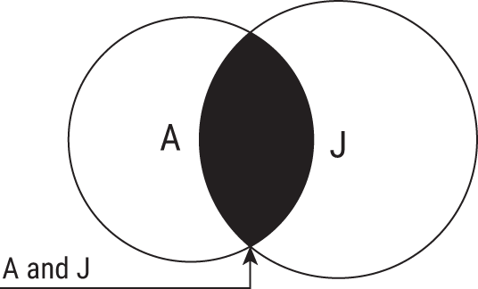
FIGURE 6.1 Venn diagram showing the probability of two events happening together cannot be greater than either event by itself.
Let's return to your truant authors for a slightly harder example. Instead of asking when Alex and Jordan will both be late to work, what about the probability that Alex or Jordan will be late? This is denoted P(A or J).
Here's what you know. P(A) = 5% and P(J) = 10%. A first guess might be P(A) + P(J) = 15%, a reasonable start. Out of 100 days, Alex will be late 5 days and Jordan will be late 10. Add them up to get 15 days, or 15% of 100. If the events were mutually exclusive and never occurred together, this would be correct.
Remember, however, that there's overlap when we both could be late. Figure 6.1 shows this. We are sometimes late to work because of each other, which is to say the probability that Alex is late and Jordan is late, P(A, J), is more than 0. We can't just add both probabilities, because that would double count the days when we were both late. To compensate, we have to subtract the probability when we're both stumbling into work after a late-night writing session, which was P(A, J) = 2%. That's 2 days out of 100 where we overlapped late days, giving the final count as 5 for Alex, 10 for Jordan, minus the 2 days when they overlapped: 5 + 10 – 2 = 13 and 13/100 = 13%.
With that information, we can formally give the additive rule for when one event or another happens at the same time: P(A or J) = P(A) + P(J) – P(A, J) = 5% + 10% − 2% = 13%.
That was a lot of notation, dice, coin flips, and your authors running late to work. So, to take a step back from notation and numbers, let's do a thought exercise without either.
PROBABILITY THOUGHT EXERCISE
Sam is 29 years old, reserved, and very bright. He majored in economics in his home state of California. As a student, he was obsessed with data, volunteered at the university's statistical consulting center, and taught himself how to program in Python (a computer programming language).
Which of these is more probable?
- Sam lives in Ohio.
- Sam lives in Ohio and works as a data scientist.
The correct answer is #1, even though nothing in the description suggests Sam would live in Ohio without also being a data scientist. This is a rebranding of the popular Linda problem in the book, Thinking, Fast and Slow4, and it's a problem most people get wrong. How did you do?
Did you pick #2? Perhaps it was because we gave you background into the fact that Sam knew programing and could be a data scientist. #2 seems more probable precisely because it mentions an event aligned with Sam's background, but it's still less probable than number #1.
Here's why. This example is stripped of notation and numbers, but it still reflects an important lesson in the previous section. The chance of any two events happening together can't be greater than either event happening by itself. The more “and” qualifications you add to any statement, the more you narrow the possibilities. For Sam to be a data scientist and live in Ohio, he must first live in Ohio. He might live in Ohio and work as an actuary.
Remember, the probability of two events happening together uses the multiplicative rule. The probability of Sam living in Ohio and working as a Data scientists can be represented as P(O, D) = P(O) × P(D | O). And because probabilities are no more than one, multiplying P(O), the probability Sam lives in Ohio, by any other probability can never make the resulting number, P(O) × P(D | O), increase. Thus, it's impossible for P(O, D) to ever be greater than P(O), no matter how right it felt in the moment to guess #2.
Still wrestling with it? You may have read #2 as a conditional probability: what is the probability Sam lives in Ohio given he works as a data scientist, P(O | D). This can be more probable than Sam living in Ohio, P(O); however, the language difference between “and” and “given” matters.
Take an easier example: The New York Yankees baseball team has loyal fans across the world. Suppose there's a game right now with millions watching, both at the stadium and on television. Now randomly select a person in the world. With billions of people in the world, it's very unlikely you'd pick a Yankees fan. It's even more unlikely you'd select a Yankees fan sitting at the game because not all fans can attend the game. But if you were given the ability to randomly select a person at the game, everything changes. It's highly probable they are a Yankees fan.5
Thus, the probability of a person being a Yankees fan and attending the game is vastly different from the probability of a person being a Yankees fan given they are at the game.
Next Steps
After that thought exercise, it's worth stating the warning we shared at the beginning of the chapter: be mindful and recognize that your intuition can play tricks on you. Probabilities will continue to confound and confuse. Perhaps the best we can do to combat this is point out some common traps.
In that spirit, and now that you're armed with the rules and notation of probability, we'll dedicate the rest of this chapter with sections to help you be aware and think critically about the probabilities you examine in your work. Here are some guidelines to keep you on the right track:
- Be careful assuming independence
- Know that all probabilities are conditional
- Ensure the probabilities have meaning
BE CAREFUL ASSUMING INDEPENDENCE
If events are independent, you can multiply their probabilities together: the probability of flipping two heads in a row on a fair coin is P(H) × P(H) = 1/2 × 1/2 = 1/4. But not all events are independent, and you need to be careful with this assumption when you're calculating or reviewing probabilities.
We mentioned this early in the book with the mortgage crisis of 2008. The probability of someone defaulting on their mortgage is not independent from the probability their neighbor defaults, though for many years Wall Street didn't think so. Both are intrinsically tied to the overall economy and state of the world.
Yet, assuming independence when events are not is a mistake made again and again. Your company might be making this mistake in strategy sessions. And this risk is underestimating, perhaps grossly underestimating, the probability multiple events can occur simultaneously.
Consider, for example, a C-level strategy session in a boardroom where they're placing three big bets for the company in the coming year—high-profile, exciting, but risky projects. Call the projects A, B, C. The execs know it's possible each project could fail, and estimates the probability of failure for each project as P(A fails) = 50%, P(B fails) = 25%, and P(C fails) = 10%.
Someone grabs a calculator and multiplies the probabilities: 50% × 25% × 10% = 1.25%. The execs are ecstatic—there is only a 1.25% chance all three fail. These are big bets, after all. Just one successful project will justify their investment in the three. And, because all outcomes must sum to 1, the probability at least one project will succeed would be 1 minus the probability all fail, or 1 – 0.0125 = .9875 = 98.75%. Wow, they think, almost a 99% probability of overall success!
Alas, their math is wrong. The events are dependent on the overall success of the company, which could be brought down by a host of examples: corporate scandal, poor quarterly results, or some larger event tied to the health of the global economy, like the COVID-19 pandemic. The events A, B, and C are dependent on several factors. Therefore, by wrongfully assuming independence, they are underestimating the probability all projects will fail next year, and thus overestimating the chances at least one will be successful.
Lest you think that doesn't seem important, remember the 2008 financial collapse and the ensuing recession.
Don't Fall for the Gambler's Fallacy
On the flip side, some events are independent but not viewed that way. This creates a different kind of risk that casinos thrive on, where people overestimate how likely something can occur based on recent events.
A fair coin, even if it lands on 10 heads in 10 consecutive flips, still has P(H) = 50% on the next flip. With independent events, your chances for an event do not increase or decrease based on past performance. But gamblers falsely believe the probabilities change—hence, the name Gambler's fallacy.6
Every roll of the dice is independent of the previous roll, each pull on a slot machine has no memory of the pull before, and each spin on the roulette wheel does not depend on the last. Yet gamblers fall victim to finding patterns in these events. They either think a slot machine is “due” to hit because it hasn't shot out coins in a while, or they believe the dice are “hot”—winning dice keep winning.
But each instance has the same probability of winning as the last. And since it's in a casino, the probabilities are not in your favor. But amateur gamblers bet big when a cluster of rare events occurs, thinking it's their lucky day to get paid. Oh, how wrong they are. But, hey, maybe the casino will give them a “free” breakfast buffet.7
ALL PROBABILITIES ARE CONDITIONAL
All probabilities are conditional in some way. A coin flip with P(H) = 50% is conditional on the coin being fair. Rolling a die with P(D == 1) = 1/6 is conditional on using an unloaded die. The probability of success on a data project is conditional on the collective wisdom of the data team, the correctness of data, the difficulty of the problem, whether your computer gets a virus, whether a pandemic shuts down the company, and on and on.
Think, also, about how businesses and people judge success and competence. It's usually based on past successes. Companies hire a consultant with a winning track record or the attorney who wins the most cases, or a person demands the heart surgeon with the smallest patient death rate. The consultant may make his clients' money 90% of the time, the attorney wins 80% of her cases that go to trial, and the heart surgeon's patients have a low 2% mortality rate.
Here's how they could game the probabilities. The consultant, lawyer, and surgeon can decide whether or not to participate. They have a good idea of when they'll be successful, and if the chances don't look favorable, they can say “no.” The probability of success for each is dependent on each selecting projects most likely to succeed and avoiding those that might hurt their numbers.8
You must think of all the factors behind the probability numbers you see.
Don't Swap Dependencies
Another trap to sidestep is assuming P(A | B) = P(B | A) for two events A and B. Notice how the dependencies are swapped: In one case, A depends on B. In the other, B depends on A.
Here's an example showing the two are not equal. Let event A be “Living in New York state” and event B be “Living in New York City.” P(A | B), the probability of living in New York state given that you live in New York City is quite different than P(B | A), the probability of living in New York City given you live in New York state. The former is a guarantee, P(A | B) = 1; the latter is not, as about 60% of New York state residents live outside New York City.
It's clearly a mistake in an easy example like this, but swapping the dependencies and assuming P(A | B) = P(B | A) is an error so common it was given a name and a Wikipedia article—Confusion of the Inverse.9 In fact, it's the very error you might have made in the thought exercise at the beginning of this chapter.
Let's return to that problem now.
Your company was hacked and 1% of laptops have a virus. Event + is a positive test, event − is negative, and event V is infected with the virus. You were given the following information: P(+ | V) = 99%, P(− | not V) = 99%, and P(V) = 1%. In other words, the probability of a positive test given the laptop has the virus is 99%, the probability of a negative test given the laptop does not have the virus is 99%, and the probability a random laptop has the virus is 1%.
We wanted to know the probability a computer had a virus given a positive test result, P(V | +), but this is where the “confusion of the inverse” emerged. We asked for P(V | +), not P(+ | V), yet many people, when presented with the thought exercise, guess a number close to P(+ | V) = 99%.
The probabilities P(V | +) and P(+ | V) are not the same, but they are linked through one of the most famous theorems in all of probability and statistics—Bayes' theorem.
Bayes' Theorem
Bayes' theorem, which dates back to the 1700s, is a clever way to work with conditional probabilities that's been applied everywhere from battles to finance to DNA decoding.10 Bayes' theorem states the following for two events, A and B:
Let's unpack this a little because the notation can be intimidating. More important than memorizing the formula (or any formula for that matter) is understanding what it's doing and why it's worth knowing.
Bayes' theorem enables us to relate the conditional probability of two events. The probability of event A given event B is related to the probability of event B given event A. They are not equal (that's the “confusion of the inverse”) but related by the preceding equation.
Why do people care? In practice, one of the conditional probabilities is known and people want to find the other. For example:
- Medical researchers want to know the probability a person has a positive cancer screening test given the person has cancer, P(+ | C), so they can create more accurate tests to provide treatment right away. Policy makers want to know the inverse—the probability a person has cancer given they test positive on the screening test, P(C | +), because they don't want to subject people to unnecessary cancer treatment based on a false positive (when test says “cancer” and no cancer is present).
- Prosecutors want to know the probability a defendant is guilty given the evidence, P(G | E). This depends on the probability of finding evidence given the person is guilty, P(E | G).
- Your email provider wants to know the probability an email is spam given it contains the phrase “Free Money!”, P(Spam | Money). Using historical data, it can calculate the probability an email contains the phrase “Free Money!” given that it's spam, P(Money | Spam). (You'll learn more about this example in Chapter 11.)
- Returning to the thought exercise, you want to know the probability of your computer having a virus given a positive test, P(V | +). You know the inverse, the probability of a positive test given a computer has the virus, P(+ | V).
All these examples are linked through Bayes' theorem—a slick way to flip the conditional probabilities. That's the good news. The bad news, or rather challenging news, is that the actual calculation of some of the pieces in Bayes' theorem can be a pain. Not all probabilities are easy to come by. For instance, the rate at which a person might have cancer given they've tested positive in a cancer screening test might be easier to find out than the incidence a person has cancer given that they failed the first preliminary test.

FIGURE 6.2 Tree diagram for scanning computers for a virus at a large company
One way to assess whether you have enough information to use Bayes11 is by building a tree diagram (see Figure 6.2). We'll use the thought exercise as an example and finally reveal why the correct answer is 50%. Suppose there are 10,000 laptops in the company. We will use the implied understanding that if 99% of computers with a virus test positive, 1% will test negative, P(− | V) = 1%. Likewise, since 99% of laptops without the virus will test negative, 1% of laptops without the virus will test negative, P(+ | not V) = 1%.
Starting with 10,000 laptops, as shown in Figure 6.2, and the information we provided, you can see how they split into the four final groups: laptops with the virus that tested negative or positive and laptops without the virus that test negative or positive. Let's consider what this means. If you look at the tree diagram, you'll notice there are only two possible branches we're interested in. The first case is having the virus and testing positive—that's 99 laptops. The second case is not having the virus but still testing positive—also 99 laptops. These are called false positives.
Here's the deal: we already know the computer came back with a positive test. That means you can only be in one of these two groups. You don't know which one you are in, but if you were to pretend each laptop were a marble, and were to select one blindly from a bag, you'd have a 50% shot of being in either group because they're both the same size.
Let's plug the pieces into Bayes' theorem and see if the math matches our (new) intuition. We start with Bayes but use the events V and + instead of A and B: P(V | +) × P(+) = P(+ | V) × P(V). Next, we fill in the probabilities we know:
Doing some rearranging of P(V | +) × P(+) = P(+ | V) × P(V), we have:
That's a lot of math, but we've arrived at the answer: the probability your laptop has the virus given the positive test is 50%.
ENSURE THE PROBABILITIES HAVE MEANING
We've immersed you with numbers and notation through this chapter, especially in the previous section. But now let's take another step back and discuss how to think about and how to use probabilities.
Calibration
When probabilities are defined, they should have meaning.
For instance, assuming equal costs and benefits, a project with a 60% chance of success carries more risk than a project with a 75% chance.
We know this seems obvious, but people often take probabilities like 60% and 75% and mentally cast them as highly probable because they are more than 50%. But if this were the case, the probabilities would not be meaningful—they would have been reduced to binary decisions, either an event happened or not, which completely bypasses the point of thinking statistically and dealing with uncertainty.
Moreover, if the probability of an event is 75%, it should happen about 75% of the time.12 Again, this seems obvious, but it gives your probability meaning. It's a concept called calibration. “Calibration measures whether, over the long run, events occur about as often as you say they're going to occur.”13
Poor calibrations make it impossible to accurately assess risk. If you're a hot-shot lawyer who thinks you're going to win a case with a 90% probability, but historically has only won 60% of cases, you are poorly calibrated and overestimating your chance of success.
So, we say again, probabilities should have meaning. Realize rare events are not impossible and highly probable events are not guarantees.
Rare Events Can, and Do, Happen
A rare event might not happen to you or anyone you know, but it doesn't mean it won't happen at all. Still, we're not always well adjusted to understand events that happen infrequently.
It's true: you are unlikely to win that large jackpot lottery, but the reality is that people do win. When you consider the number of lotteries held around the world every single day, the chances that such a rare event might occur to someone on this earth is not so unrealistic, even if you're not the lucky one.
We often forget the sheer amount of people who live on this planet. With our population on the order of billions, “1 in a million” events seem far more likely to happen. Such events, in fact, capture a lot more people than we can easily comprehend. In a world with 7.8 billion people, a “1 in a million” daily event would happen to 7,800 people per day.
On the flipside, it's very easy to qualify an activity to the point that it feels rare if only (and perhaps misleadingly) to add a sense of drama. American football, for instance, is filled with heavily qualified commentary suggesting the rarity of an event unfolding on the screen. “This is the first time a 28-year-old rookie has run for 30 yards, after two away games and playing only once in the pre-season.” If you put it like that, then yes, it does perhaps seem like an infrequent occurrence.
CHAPTER SUMMARY
This chapter was not only a quick lesson in probability but also a lesson in humility. Probability is hard. But a big part in learning a new topic is respecting that things can go wrong. The information you've learned here will help you seek out additional information before making decisions about probability, especially with decisions that seem intuitive at first but now, we hope, you're suspect of.
In this chapter, we demonstrated how easy it is to misunderstand probabilities. This misunderstanding sometimes comes down to how we word a question—or the assumptions we have behind the information being given. To avoid misunderstandings, remember our guidance when seeing probabilities:
- Be careful assuming independence
- Know that all probabilities are conditional
- Ensure the probabilities have meaning
NOTES
- 1 Paulos, J. A. (1989). Innumeracy: Mathematical Illiteracy and Its Consequences (1st ed.). Hill and Wang.
- 2 Search online for “Probability Interpretations” to see what we're talking about.
- 3 Can you really be late if you work for yourself? For this example, yes.
- 4 Kahneman, D. (2013). Thinking, Fast and Slow (1st ed.). Farrar, Straus and Giroux.
- 5 Not 100% because the opposing team will also have fans at the game.
- 6 The belief that past independent events might occur given enough time is also sometimes called the “law of averages,” a scientific sounding name for wishful thinking.
- 7 The authors have nothing against breakfast buffets.
- 8 To be clear, we are not saying consultants or surgeons do this. Just attorneys.
- 9 Confusion of the Inverse: en.wikipedia.org/wiki/Confusion_of_the_inverse. Accessed on July 4, 2020.
- 10 For a complete and excellent history about Bayes' theorem, check out the book McGrayne, S. B. (2011). The Theory That Would Not Die: How Bayes' Rule Cracked the Enigma Code, Hunted Down Russian Submarines, and Emerged Triumphant from Two Centuries of Controversy (American First ed.). Yale University Press.
- 11 Here, we say “using Bayes” as a shorthand for “applying Bayes' Theorem.”
- 12 We say “about” because there's variation in all things. But in the long run, a 75% event should occur 75% of the time.
- 13 fivethirtyeight.com/features/when-we-say-70-percent-it-really-means-70-percent