
4
Advanced Python
In the previous chapter, we got acquainted with the basics of Python programming syntax. While there was nothing specific to MicroPython and Micro:bit, the knowledge we learned is like a Swiss Army knife that can be used in every Python programming project.
In this chapter, we will continue our journey of exploring Python syntax. In the final part of this chapter, we will also explore some MicroPython- and Micro:bit-specific functionality. We will explore the following list of topics together:
- Lists, tuples, and dictionaries
- Functions
- Recursion
- Object-oriented programming with Python
- Getting help for built-in modules
- Retrieving system properties with code
Let’s explore advanced concepts in programming.
Technical requirements
This chapter does not require any additional hardware. A Micro:bit board, a computer, and a micro USB cable are enough to follow the demonstrations mentioned in the chapter.
Lists, tuples, and dictionaries
Python comes with a lot of built-in data structures. In this section, we will explore a few of them. We will use the shell (REPL) for this. Let’s get started with lists. Lists can store more than one item. They are defined with square brackets, and a comma separates their elements. Lists are mutable. This means that we can change the items in lists. They also allow duplicates. Open the REPL of the IDE of your choice and start following the examples:
>>> office_suites = ["Microsoft Office", "LibreOffice", "Apache OpenOffice", "FreeOffice", "WPS Office", "Polaris Office", "StarOffice", "NeoOffice", "Calligra Suite", "OnlyOffice"]
We can see the values in the dictionary on the REPL shell console by typing in the name of the list as follows:
>>> office_suites
['Microsoft Office', 'LibreOffice', 'Apache OpenOffice', 'FreeOffice', 'WPS Office', 'Polaris Office', 'StarOffice', 'NeoOffice', 'Calligra Suite', 'OnlyOffice']
We can also use the print() method as follows:
>>> print(office_suites)
['Microsoft Office', 'LibreOffice', 'Apache OpenOffice', 'FreeOffice', 'WPS Office', 'Polaris Office', 'StarOffice', 'NeoOffice', 'Calligra Suite', 'OnlyOffice']
We can also access the individual elements of a list using the C-style indexing scheme. The index of a list with n number of items starts at 0 and ends at n-1:
>>> office_suites[0]
'Microsoft Office'
>>> office_suites[1]
'LibreOffice'
>>> office_suites[6]
'StarOffice'
We can use the built-in len() method as follows to find out the length of the list:
>>> len(office_suites)
10
We can access the final and the penultimate elements of the list as follows:
>>> office_suites[-1]
'OnlyOffice'
>>> office_suites[-2]
'Calligra Suite'
If we try to access a nonexistent element, we get the following error:
>>> office_suites[13]
Traceback (most recent call last):
  File "<stdin>", line 1, in <module>
IndexError: list index out of range
We can also create lists with the following alternative syntax:
>>> office_suites = list (('Microsoft Office', 'LibreOffice', 'Apache OpenOffice', 'FreeOffice', 'WPS Office', 'Polaris Office', 'StarOffice', 'NeoOffice', 'Calligra Suite', 'OnlyOffice'))
>>> office_suites
['Microsoft Office', 'LibreOffice', 'Apache OpenOffice', 'FreeOffice', 'WPS Office', 'Polaris Office', 'StarOffice', 'NeoOffice', 'Calligra Suite', 'OnlyOffice']
We can access a range of elements from the list:
>>> office_suites[2:5]
['Apache OpenOffice', 'FreeOffice', 'WPS Office']
We can also access all the elements after a particular index:
>>> office_suites[2:]
['Apache OpenOffice', 'FreeOffice', 'WPS Office', 'Polaris Office', 'StarOffice', 'NeoOffice', 'Calligra Suite', 'OnlyOffice']
We can access all the elements before an index:
>>> office_suites[:2]
['Microsoft Office', 'LibreOffice']
We can change an element at a specific index as follows:
>>> office_suites[0] = 'GNOME Office'
We can insert an item at a particular index, and the items after that index will be automatically shifted:
>>> office_suites.insert(2, 'SoftMaker Office')
We can append an item at the end of the list:
>>> office_suites.append('Microsoft Office')We can remove an item of a particular value from the list as follows:
>>> office_suites.remove('Microsoft Office')We can iterate over a list using a for loop as follows. Save the following code as a Python program and run it:
office_suites = list (('Microsoft Office', 'LibreOffice',
                       'Apache OpenOffice', 'FreeOffice',
                       'WPS Office', 'Polaris Office',
                       'StarOffice', 'NeoOffice',
                       'Calligra Suite', 'OnlyOffice'))
for i in office_suites:
    print(i)
Similarly, we can employ a while loop for the same purpose as follows:
office_suites = list (('Microsoft Office', 'LibreOffice',
                       'Apache OpenOffice', 'FreeOffice',
                       'WPS Office', 'Polaris Office',
                       'StarOffice', 'NeoOffice',
                       'Calligra Suite', 'OnlyOffice'))
i = 0
while i < len(office_suites):
    print(office_suites[i])
    i = i + 1
Let’s have a brief look at the concept of tuples. Tuples are immutable in nature. This means that once created, they cannot be changed. We can use tuples to store constant arrays of values. The following is an example of tuples:
>>> languages = ('C', 'C++', 'Python')Just like lists, we can access languages using indices:
>>> languages[0]
'C'
>>> languages[-1]
'Python'
We can demonstrate the immutability of tuples by trying to change a value as follows:
>>> languages[1] = 'Java'
We get the following error:
Traceback (most recent call last):
  File "<stdin>", line 1, in <module>
TypeError: 'tuple' object doesn't support item assignment
Let’s understand the concept of dictionaries. Dictionaries are ordered, mutable (changeable), and do not allow duplicates. Items are stored in dictionaries in pairs of keys and values. The following is an example of a simple dictionary:
>>> dev_env = {"language" : "C", "compilers": ['GCC', 'llvm', 'MinGW-w64', 'VC++']}
>>> dev_env
{'compilers': ['GCC', 'llvm', 'MinGW-w64', 'VC++'], 'language': 'C'}
We can access a value using its key as follows:
>>> dev_env['language']
'C'
>>> dev_env['compilers']
['GCC', 'llvm', 'MinGW-w64', 'VC++']
We can also retrieve all the keys and all the values, respectively, as follows:
>>> dev_env.keys()
dict_keys(['compilers', 'language'])
>>> dev_env.values()
dict_values([['GCC', 'llvm', 'MinGW-w64', 'VC++'], 'C'])
We can update/change a value as follows:
>>> dev_env.update({"language": "C++"})
>>> dev_env
{'compilers': ['GCC', 'llvm', 'MinGW-w64', 'VC++'], 'language': 'C++'}
We can also add a pair of keys and values as follows:
>>> dev_env['OS'] = ["UNIX", "FreeBSD", "Linux", "Windows 11"]
>>> dev_env
{'compilers': ['GCC', 'llvm', 'MinGW-w64', 'VC++'], 'OS': ['UNIX', 'FreeBSD', 'Linux', 'Windows 11'], 'language': 'C++'}
This is how we can work with lists, tuples, and dictionaries. Next, let’s look at functions.
Functions
Let’s understand the concept of functions. They are also called subroutines. They are a common programming practice. If a block of code is too long and repetitively used in the program, then we write that block separately from the other code and assign it a name. We call the block using the assigned name wherever needed. Let’s see an example:
def message():
    name = input("What is your name, My liege : ")
    print("Ashwin is your humble servant, My liege " + name)
print("First function call...")
message()
print("Second function call...")
message()
In this example, we have defined our own function and named it message(). The definition of the function begins with the def keyword. The output is as follows:
>>> %Run -c $EDITOR_CONTENT
First function call...
What is your name, My liege : Henry V
Ashwin is your humble servant, My liege Henry V
Second function call...
What is your name, My liege : Caesar
Ashwin is your humble servant, My liege Caesar
This is a very simple example. We can also define a function with parameters, and we can pass arguments to those parameters in the function call as follows:
def printHello( first_name ):
    print("Hello {0}".format(first_name))
def printHello1( first_name, last_name ):
    print("Hello {0}, {1}".format(first_name, last_name))
def printHello2( first_name, msg='Good Morning!'):
    print("Hello {0}, {1}".format(first_name, msg))
printHello('Ashwin')
printHello(first_name='Thor')
printHello1('Ashwin', 'Pajankar')
printHello1(first_name='Ashwin', last_name='Pajankar')
printHello1(last_name='Pajankar', first_name='Ashwin')
printHello1('Thor', 'Odinson')
printHello2('Ashwin', 'Good Evening!')
printHello2('Thor')
The first definition is a very basic example. In the second definition, we are defining a function with multiple parameters. In the third definition, we are defining a function with the default argument.
We have tried different ways to call the functions. Sometimes, we have mentioned the names of the parameters. We have also changed the order of the parameters in the function call. Also, we have tried the function call with the default arguments. The following is the output:
>>> %Run -c $EDITOR_CONTENT
Hello Ashwin
Hello Thor
Hello Ashwin, Pajankar
Hello Ashwin, Pajankar
Hello Ashwin, Pajankar
Hello Thor, Odinson
Hello Ashwin, Good Evening!
Hello Thor, Good Morning!
Perhaps it is a good idea to change the arguments and their order in the function call to understand this concept better. Try that yourself as an exercise.
A function can also be defined as returning a value or multiple values. We can store these values in variables. The following is a simple example:
def square(a):
    b = a**2
    return b
def power(a, b):
    return a**b
def multiret(a, b):
    a += 1
    b += 1
    return a, b
num = square(3)
print(num)
num = power(3, 3)
print(num)
x, y = multiret(3, 5)
print("{0}, {1}".format(x, y))
The output is as follows:
>>> %Run -c $EDITOR_CONTENT
9
27
4, 6
We can also define a function to accept an arbitrary number of arguments as follows:
def team( *members ):
    print("
My team has following members :")
    for name in members:
        print( name )
team('Ashwin', 'Jane', 'Thor', 'Tony')
team('Ashwin', 'Jane', 'Thor')
in print() refers to a newline. It prints the entire string on the next line. The output is as follows:
>>> %Run -c $EDITOR_CONTENT
My team has following members :
Ashwin
Jane
Thor
Tony
My team has following members :
Ashwin
Jane
Thor
Let’s learn about global and local variables now. A variable can be created outside and inside a function. The variable created inside a function is known as a local variable, and its scope is limited to that function, whereas a global variable can be accessed anywhere. The following program demonstrates a global and a local variable:
x = "Python"
def function01():
  x = "C++"
  print(x + " is the best language.")
function01()
print(x + " is the best language.")
In the preceding program, the x variable defined outside function01() is a global variable. The x variable defined inside function01() is a local variable of that function. The output is as follows:
>>> %Run -c $EDITOR_CONTENT
C++ is the best language.
Python is the best language.
We can also access the global variable inside a function as follows:
x = "Python"
def function01():
  global x
  print(x + " is the best language.")
function01()
Run the program and check the output. In the following section, we will study another important concept, recursion.
Recursion
In Python, just like many other programming languages, a defined function can call itself. This is known as recursion. A recursive pattern has two important components. The first is the termination condition, which defines when to terminate the recursion. In the absence of this or if it is erroneous (never meets the termination criteria), the function will call itself an infinite number of times. This is called infinite recursion. The other part of the recursion pattern is recursive calls. There can be one or more of these. The following program demonstrates simple recursion:
def print_message(string, count):
    if (count > 0):
        print(string)
        print_message(string, count - 1)
print_message("Hello, World!", 5)
In the preceding program, we use recursion in place of a for or while loop to print a message repetitively.
Let’s write a program for computing a factorial as follows:
def factorial(number):
    if number < 0:
        print("The number must be greater than zero.")
        return -1
    elif ((number - int(number)) > 0):
        print("The number must be a positive integer.")
        return -1
    elif (number == 0) or (number == 1):
        return 1
    else:
        return number * factorial(number-1)
factorial(-1)
factorial(1.1)
print(factorial(0))
print(factorial(1))
print(factorial(5))
The output is as follows:
The number must be greater than zero.
The number must be a positive integer.
1
1
120
The following program employs recursion to return the number in the Fibonacci sequence at the given index:
def fibonacci(number):
    if number <= 1:
        return number
    else:
        return fibonacci(number-1) + fibonacci(number-2)
print(fibonacci(3))
Indirect recursion
The type of recursion we have seen in the preceding three examples is known as direct recursion because the recursive function calls itself. We can write our program with two or more functions calling each other, creating something we call indirect recursion. The following is an example of a ping-pong mechanism demonstrated with indirect recursion:
def ping(i):
    if i > 0:
        print("Ping - " + str(i))
        return pong(i-1)
def pong(i):
    if i > 0:
        print("Pong - " + str(i))
        return ping(i-1)
ping(10)
The output is as follows:
Ping - 10
Pong - 9
Ping - 8
Pong - 7
Ping - 6
Pong - 5
Ping - 4
Pong - 3
Ping - 2
Pong – 1
This is how we can work with recursion. In the next section, we will briefly have a look at the concepts of the object-oriented programming paradigm in Python.
Object-oriented programming with Python
This is one of the most important sections in the chapter. The object-oriented programming paradigm revolves around the concept of objects. Objects contain data (in the form of properties) and functions (in the form of procedures, known as methods in Python programming). We will use a lot of these concepts in our projects. Let’s create an integer variable as follows:
>>> a = 10
We can use the built-in type() method to see the data type of the variable as follows:
>>> type(a)
<class 'int'>
We can do this for the other types of values, too, as follows:
>>> type("Hello, World!")
<class 'str'>
>>> type(3.14)
<class 'float'>
This means that everything is an object in Python. An object is a variable of a class data type. These classes could be built-in library classes or user-defined classes. Let’s see a simple example of a user-defined class as follows:
class fruit:

    def __init__(self, str):
        self.name = str

    def printName(self):
        print(self.name)
f1 = fruit('Mango')
print(type(f1))
f1.printName()
The output is as follows:
>>> %Run -c $EDITOR_CONTENT
<class 'fruit'>
Mango
We are using the class keyword to define a user-defined class. The constructor or initializer is defined with __init__ and is called implicitly when we create an object of the class. The variable name is a property of the class. The function defined within a class is known as a method or a class method. printName() is one such class method. For practice, create your own classes to represent real-life concepts. For example, a class corresponding to a computer can have properties, such as processor name, processor speed, RAM type, RAM size, graphics card model, and so on. It can also have methods such as powerOff(), powerOn(), and reset().
We can also use the classes created in one program in another program. Basically, a Python code file is also known as a module. And we can use the import keyword to use such modules in other Python programs. We will use plenty of such standard Python and MicroPython library modules for the demonstrations in this book.
The object-oriented programming paradigm is a vast topic, and it is not feasible to cover it entirely in a single chapter. So, we will explore only the features that are relevant to programming a Micro:bit.
Exploring the random module
Let’s generate random numbers with a built-in random() module. Type the following code in to the REPL shell:
>>> import random
This imports the module to our shell (or Python program). The module has many methods. We will see a few important ones. We can obtain any random float between 0.0 and 0.1 with the random() method as follows:
>>> random.random()
0.2952699
We can obtain a random integer in the given range with the randint() method as follows:
>>> random.randint(2, 5)
4
We can obtain a random number (a floating point number) in the given range with the uniform() method as follows:
>>> random.uniform(2, 5)
3.330382
In the case that we do not wish to use the name of the module with the method, we have to import in the module the following way:
>>> from random import *
The following is a program that demonstrates this style of coding:
from random import *
print(random())
print(randint(2, 5))
print(uniform(2, 5))
We will use both styles of coding in this book.
In the next section, we will explore how to get help for the built-in library modules in Python.
Getting help for built-in modules
We can get help for the built-in modules with the following command in the REPL shell:
>>> help('modules')This shows the list of all the available modules as follows:
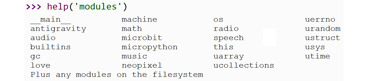
Figure 4.1 – Built-in modules
Note that the output is interpreter-specific. The preceding screenshot (Figure 4.1) shows the output specific to the MicroPython interpreter implemented for the Micro:bit. If we run the same statement on any other interpreter of Python (for example, CPython, the reference implementation interpreter of Python by the Python Software Foundation), we will see a different list.
We can mention the name of any built-in module as an argument to the help() method to see the details of the module as follows:

Figure 4.2 – Obtaining help
All the code we have practiced before now in this chapter and the previous one can be executed with the standard reference implementation of Python 3 (www.python.com). As an exercise, execute all the statements and programs on the IDLE shell interpreter.
Retrieving system properties with code
Now, let us see some Micro:bit-specific MicroPython code. This code is only run on MicroPython running on the Micro:bit. It won’t run on the standard Python 3 interpreter. Let’s see the properties of our Micro:bit device as follows:
# micro:bit specific MicroPython code
import machine
print("Unique ID : " + str(machine.unique_id()))
print(str(machine.freq()/1000000) + " MHz")
The program prints the unique ID and the frequency of our Micro:bit board. The following is the output:
>>> %Run -c $EDITOR_CONTENT
Unique ID : b'$xd1xb4[xe2a?xd5'
64.0 MHz
This is how we can fetch and display system properties.
Summary
In this chapter, we explored the advanced features of the Python programming language. The final program was specific to MicroPython running on a Micro:bit. From the next chapter onward, all the code demonstrations will be specific to MicroPython running on a Micro:bit, and they will not run on any Python 3 implementation.
After completing this chapter, you will understand the power of the Python programming language. It is simple yet concise and powers devices such as the Micro:bit and other microcontrollers (such as the Raspberry Pi Pico W and ESP32) in the form of MicroPython. Anyone can learn to work with Python and MicroPython. The following is a photograph of my neighbors in my village working on a Micro:bit connected with NeoPixel Ring (we will fully explore this in Chapter 11, Working with NeoPixels and a MAX7219 Display) for their school project:
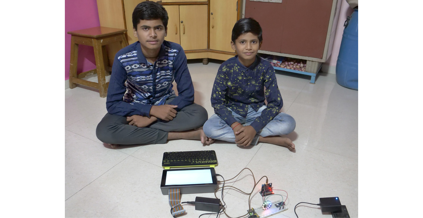
Figure 4.3 – Schoolkids working on a NeoPixel with a Micro:bit
From the next chapter onward, we will start creating projects with hardware programming. In the next chapter, we will explore how to program a built-in LED matrix and push buttons in depth.
Further reading
The basics we have learned about up to now are available in the format of video tutorials on YouTube on my channel at https://www.youtube.com/watch?v=PITLKocdY14&list=PLiHa1s-EL3vhJTNPXOkjsWDes9cMZRolD. I have used Micro:bit V1 for recording the tutorials. However, they are not outdated. All the videos are consolidated into a single lecture at https://www.youtube.com/watch?v=YcHZj_B6X18. It will be worth exploring these tutorials.