6

Surfaces - The First Foundational Component to Designs within Civil 3D

Within any Civil 3D design, surfaces, alignments, and profiles are often considered the three major foundational components required to build a true Civil infrastructure design model. In Chapter 4, Configuring Survey Data with Civil 3D, we were afforded the benefits of having our survey data already being converted to 2D and 3D geometry, making up our survey model.

In Chapter 5, Leveraging Points, Lines, and Curves, we reviewed many of the preparational tasks that we need to perform to process surveyed data into 2D geometry to be displayed in our survey model.

In this chapter, we’ll begin by focusing on surfaces as the root foundation 3D component that we will use to reference and build additional 3D components from. That said, key topics that will be covered in this chapter include the following:

• Generating a surface model
• Understanding surface styles
• Surface manipulation and management

Leveraging the survey point data and point groups we created in Chapter 5, Leveraging Points, Lines, and Curves, we’ll pick up where we left off by opening the Survey Model.dwg file located in the Practical Autodesk Civil 3D 2024Chapter 6 subfolder.

Technical requirements

The exercise files for this chapter are available at https://packt.link/UoiPn

Generating a surface model

If you recall, in Chapter 5, Leveraging Points, Lines, and Curves, we created point groups for each of our survey points and processed them into linework, with the exception of our Ground Point Group. In this section, we’ll use Ground Point Group to generate a 3D surface model that we will use as a reference for building our design.

To kick things off, we’ll start by going into TOOLSPACE, selecting the Prospector tab, and locating the Surfaces category. If we right-click on Surfaces, we will be presented with the following options, also displayed in Figure 6.1:

• Create Surface…: Provides the ability to create a new surface model (TIN, Grid, TIN Volume, or Grid Volume)
• Create Surface From DEM…: Provides the ability to create a new surface model (via USGS Digital Elevation Model (DEM)), GEOTIFF, ESRI ASCII Grid, or ESRI Binary Grid)
• Create Surface from TIN…: Provides the ability to create a new surface model from a TIN file
• Show Preview: When Show Preview is enabled, or checked, a preview of the individual modeled object will display at the bottom of our Toolspace dialog box
• Rebuild Out of Date Items: Rebuilds surface models if a component applied to the surface definition has been updated
• Create Folder: Provides the ability to manage surfaces at a level deeper by adding folder creation capabilities
• Export to DEM: Exports all surface models to any of the following formats: DEM and GEOTIFF
• Export to LandXML: Exports all surface models to a LandXML file
• Refresh: Refresh

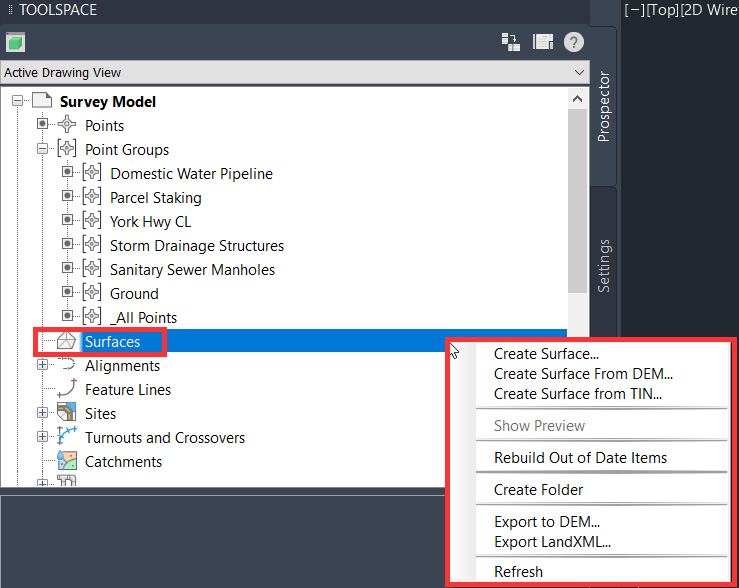
Figure 6.1 – Right-click options for Surfaces

To ensure that we are keeping our surface models organized, we’ll go ahead and select the Create Folder option. In the Create Folder dialog box, set New folder name to Existing Conditions, as shown in Figure 6.2:

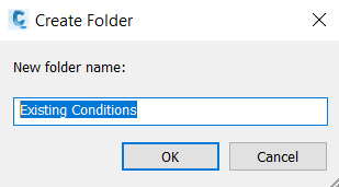
Figure 6.2 – Create Folder dialog box

Going back to the Surfaces category, right-click again on Surfaces but select the Create Surface option this time. When the Create Surface dialog box appears, we’ll make the following selections (also shown in Figure 6.3):

• Type: TIN surface (the type of surface model we wish to create).
• Surface Layer: C-TOPO (the layer on which our surface model as a whole will be placed).
• Name: SRF - Existing Grade – FromSurveyPoints (naming conventions are important to define at the beginning to drive consistency and make things clear as to what each component represents. In this case, SRF represents Surface, Existing Grade – FromSurveyPoints and indicates that this particular component represents the overall existing surface model and has been generated from survey point data.
• Description: Created from Ground Point Group (it’s always good practice to add a description and clarifying statements as to how the surface model was constructed).
• Style: Contours 2’ and 10’ (Background) (represents the style that will be applied to our surface model that will appear in our plan views).
• Render Material: ByLayer (represents the style that will be applied to our surface model that will appear in 3D views).

Figure 6.3 – Create Surface dialog box

Once all the fields have been filled out accordingly, click the OK button. Going back to the TOOLSPACE | Prospector tab, let’s go ahead and select our newly created surface and drag and drop it into the Existing Conditions folder, as shown in Figure 6.4:

Figure 6.4 – Create Surface dialog box

Click on the + icon next to the SRF - Existing Grade – FromSurveyPoints surface model along with the + icon next to Definition. With these expanded, we can now begin adding components to our existing surface model. As we add components, these will update in our model space, so keep an eye out for these updates occurring.

As it relates to components, we are able to add to the surface definition here. We have the following options available to us:

• Boundaries: Allows us to apply Outer, Show and Hide, and Data Clip boundaries to our surface models
• Breaklines: Allows us to apply Standard, Proximity, Wall, From File, and Non-Destructive Breaklines to our surface models
• Contours: Allows us to apply existing polylines representing manually placed contours to our surface models
• DEM Files: Allows us to apply external USGS DEM, GEOTIFF, ESRI ASCII Grid, or ESRI Binary Grid files to our surface models
• Drawing Objects: Allows us to apply AutoCAD Points, Lines, Blocks, Text, 3D Faces, and Polyfaces to our surface model
• Edits: Allows us to perform various edits to our surface model (that is, modifying TIN lines, Adding/Deleting Points, Minimizing Flat Areas, Smoothing Surfaces, and Simplifying Surfaces)
• Point Files: Allows us to apply an external Point File (in .txt, .prn, .csv, .auf, .nez, .pnt format) to our surface model
• Point Groups: Allows us to apply Point Group to our surface model
• Point Survey Queries: Allows us to apply and generate a dynamic link to survey points (typically used in surveying workflows)
• Figure Survey Queries: Allows us to apply and generate a dynamic link to survey figures (typically used in surveying workflows)

For the purposes of our SRF - Existing Grade – FromSurveyPoints surface model, we want to apply Point Groups to our surface definition. That said, let’s right-click on the Point Groups option and select Add, as shown in Figure 6.5:

Figure 6.5 – Add Point Groups to surface definition

We’ll then be presented with a Point Groups dialog box where we can then select the point groups created in our current survey model file from which we can build our SRF - Existing Grade – FromSurveyPoints surface model.

In our case, we’ll obviously want to select the Ground point group, click Apply, and then OK, as shown in Figure 6.6:

Figure 6.6 – Point Groups dialog box

After clicking OK in the Point Groups dialog box, we’ll notice that the SRF - Existing Grade – FromSurveyPoints surface model has now appeared in our model space and is displayed using the 2’ and 10’ (Background) display style we applied at the initial creation, as shown in Figure 6.7:

Figure 6.7 – SRF - Existing Grade – FromSurveyPoints surface model

We have now officially created our very first surface model within Civil 3D and have a great foundation from which to build our design! We can now begin exploring different ways we can view, analyze, manipulate, and manage our surface model moving forward.

Understanding surface styles

Importing our survey data and creating our surface models for sheet preparation is one thing (which we accomplished in the previous section). Understanding what we’re looking at by applying different surface styles is a completely different ballgame.

In this section, we’ll familiarize ourselves with the various surface styles available to us and learn how to display our surfaces under different circumstances.

For this section, let’s leave the Survey Model.dwg file and open the Survey Model_DisplayStyles_Start.dwg file located in the Practical Autodesk Civil 3D 2024Chapter 6 subfolder. Once it’s open, you will notice that it should look very similar to where we left off in the Survey Model.dwg file.

Note

Since we will be running various tests on the new file we have opened, it’s best practice to leave the original as is to avoid introducing any type of file corruption. The common practice for setting up these types of testing environments is to simply perform a Save As (type this on the command line) and save it as the same name with Working at the end. Adding this suffix to the drawing name will notify users that this file is for testing purposes and not meant to be a final drawing.

In the current Survey Model_DisplayStyles_Start.dwg file, let’s go over to TOOLSPACE, select the Settings tab, and expand the Surface category by clicking the + icon next to Surface.

Notice that we have the following list of subcategories associated with surfaces (also displayed in Figure 6.8):

• Surface Styles: Here, we can view the comprehensive list of available display styles associated with surface models.
• Label Styles: Here, we can view the comprehensive list of available label styles that can be applied to our surface models for annotation purposes; these can also display specified symbology.
• Table Styles: Here, we can view the comprehensive list of available table styles that can be displayed for sheeting purposes as they relate to our surface models.
• Commands: Here, we can view the comprehensive list of available commands that can simply be typed into the command line to perform specific tasks associated with surfaces.

Figure 6.8 – TOOLSPACE | Settings tab – surface styles expanded

Starting with surface styles, if we click on the + icon next to Surface Styles, we will then see the comprehensive list of options that reside in our current drawing.

Note

These are also contained within the Company Template File.dwt drawing template that we created as a starting point for new files. All styles listed from here on will be included in any new file, provided you are using the Company Template File.dwt drawing template as the base.

Once expanded, we’ll see the following list of surface styles that can be applied to our surface models, within our current file, for display purposes (also refer to Figure 6.9):

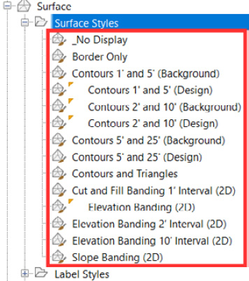
Figure 6.9 – Surface Styles

• _No Display: Applying this display to our surface model will turn all components off in model space.
• Border Only: Applying this display to our surface model will only turn on the border(s) within model space.
• Contours 1’ and 5’ (Background): Applying this display to our surface model will only turn on minor and major contours at 1' intervals in model space. Contours displayed will be assigned to layers that have grey assignments, so they are screened when plotted.
• Contours 1’ and 5’ (Design): Applying this display to our surface model will only turn on minor and major contours at 1' intervals in model space. Contours displayed will be assigned to layers that have brighter color assignments so they are more prominent when plotted.
• Contours 2’ and 10’ (Background): Applying this display to our surface model will only turn on minor and major contours at 2' intervals in the model space. Contours displayed will be assigned to layers with gray assignments, so they are screened when plotted.
• Contours 2’ and 10’ (Design): Applying this display to our surface model will only turn on minor and major contours at 2' intervals in the model space. Contours displayed will be assigned to layers that have brighter color assignments so they are more prominent when plotted.
• Contours 5’ and 25’ (Background): Applying this display to our surface model will only turn on minor and major contours at 5' intervals in the model space. Contours displayed will be assigned to layers with gray assignments, so they are screened when plotted.
• Contours 5’ and 25’ (Design): Applying this display to our surface model will only turn on minor and major contours at 5' intervals in the model space. Contours displayed will be assigned to layers that have brighter color assignments so they are more prominent when plotted.
• Contours and Triangles: Applying this display to our surface model will turn on the triangles and border(s), along with the minor and major contours at 2' intervals in model space. Elements displayed will be assigned to layers with gray assignments so they are screened when plotted.
• Cut and Fill Banding 1’ Interval (2D): Applying this display to our surface model will only turn on elevations, where the color scheme displayed in model space is initially identified by the default settings applied in Surface Style | Analysis | Elevations | Range color scheme (refer to Figure 6.10).

Figure 6.10 – Surface Style properties | Analysis tab | Elevations default settings

• Elevation Banding (2D): Applying this display to our surface model will only turn on elevations, where the color scheme displayed in the model space is initially identified by the default settings applied in Surface Style | Analysis | Elevations | Range color scheme (refer to Figure 6.10).
• Elevation Banding 2’ Interval (2D): Applying this display to our surface model will only turn on elevations, where the color scheme displayed in the model space is initially identified by the default settings applied in Surface Style | Analysis | Elevations | Range color scheme (refer to Figure 6.10).
• Elevation Banding 10’ Interval (2D): Applying this display to our surface model will only turn on elevations, where the color scheme displayed in model space is initially identified by the default settings applied in Surface Style | Analysis | Elevations | Range color scheme (refer to Figure 6.10).
• Slope Banding (2D): Applying this display to our surface model will only turn on elevations, where the color scheme displayed in the model space is initially identified by the default settings applied in Surface Style | Analysis | Elevations | Range color scheme (refer to Figure 6.10).

Next, we’ll visit surface label styles by clicking on the + icon next to Label Styles – at which point, we’ll see a comprehensive list of surface label styles that reside in our current drawing.

Once expanded, we’ll see the following list of Label Styles that can be applied to our surface models within our current file for annotation display purposes (for a more detailed breakdown of Label Styles in our current file, refer to Figure 6.11):

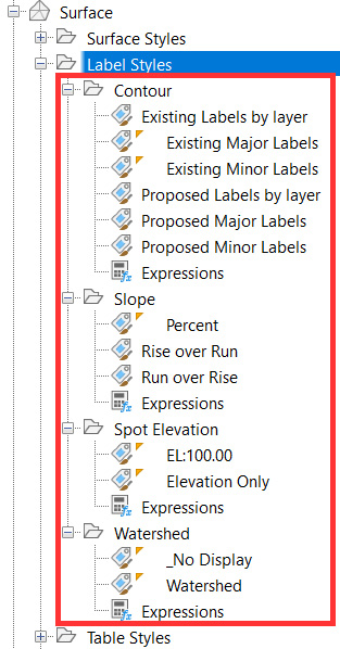
Figure 6.11 – Surface Label Styles (detailed version)

• Contour: Contour labels are displayed using the Add Surface Labels option within the Annotate ribbon (refer to Figure 6.12 for the workflow and location), provided a Surface Display Style showing contours (Minor and/or Major) are displayed as well. Please note that surface contour labels will automatically be associated with the contour interval defined in the Surface Display Style settings.
• Slope: Slope labels will be displayed in various formats as we identify locations where we would like to place them using the Slope labels option within the Annotate ribbon (refer to Figure 6.12 for workflow and location).
• Spot Elevation: Spot labels will be displayed in various formats as we identify locations where we would like to place them using the Spot Elevation option within the Annotate ribbon (refer to Figure 6.12 for workflow and location).

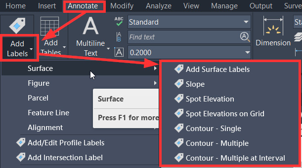
Figure 6.12 – Workflow for adding surface labels

• Watersheds: Watershed labels will be displayed as defined in the Watershed Label Properties, provided a Surface Display Style showing the watersheds is displayed as well, where the label styles displayed in model space are initially identified by the default settings applied in Surface Style | Watersheds | Surface | Surface Watershed Label Style (refer to Figure 6.13).

Figure 6.13 – Workflow for adding surface labels

Next, we’ll look at the surface table styles by clicking on the + icon next to Table Styles – at which point, we’ll then see a comprehensive list of surface table styles that reside in our current drawing as well (refer to Figure 6.11).

Note

It’s important to note that surface table styles will reference the user-defined settings applied in the Analysis tab in the Surface Properties dialog box (refer to Figure 6.14 for the location and example settings).

Figure 6.14 – Example of Analysis settings applied to our surface model

Once expanded, we’ll see the following list of Table Styles (also refer to Figure 6.15 for a detailed breakdown of the surface table styles in our current file) that can be added to our drawings for sheeting purposes.

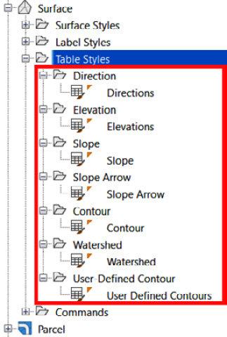
Figure 6.15 – Surface Table Styles (detailed version)

• Direction: This table style will be dynamically linked to the settings defined in Figure 6.14 and display direction ranges, colors, and area values accordingly
• Elevation: This table style will be dynamically linked to the settings defined in Figure 6.14 and display elevation ranges, colors, area, and volume values accordingly
• Slope: This table style will be dynamically linked to the settings defined in Figure 6.14 and display slope ranges, colors, and face area values accordingly
• Slope Arrow: This table style will be dynamically linked to the settings defined in Figure 6.14 and display slope arrow ranges, colors, and face area values accordingly
• Contour: This table style will be dynamically linked to the settings defined in Figure 6.14 and display contour ranges, colors, areas, and volume values accordingly
• Watershed: This table style will be dynamically linked to the settings defined in Figure 6.14 and display number, type, description, color, hatching, and drainage area values accordingly
• User-Defined Contour: This table style will be dynamically linked to the settings defined in Figure 6.14 and display user-defined contour ranges, colors, areas, and volume values accordingly

With the overview of all applicable styles that can be applied to our surfaces out of the way, let’s get a better understanding of what some of these actually mean and represent, how we can apply different styles under different circumstances and scenarios, and enhance our overall understanding of an existing conditions surface model, and any other surface model for that matter.

Surface manipulation and management

In the majority of cases, we’re going to want to display our surface model with contours displayed, where typical intervals applied would be either 1' (minor) and 5' (major) or 2' (minor) and 10' (major), depending on the complexity and the size of the site where the design will be developed from. As we work through our designs, we may want to switch our surface model display as different design elements are introduced.

For example, say we want to perform a slope analysis of the existing surface model to quickly identify any potential risks or concerns related to slope stabilization on our current site. Although there are other factors that play into these types of analysis (such as soil types, water content, and vegetation), we can get a pretty good idea of what the current conditions are by performing a simple slope analysis on our existing surface model.

To do so, let’s jump back into the Survey Model_DisplayStyles_Start.dwg file, select our surface model displayed in model space, right-click and select the Surface Properties option, as shown in Figure 6.16:

Figure 6.16 – Access Surface Properties in the model space

Once the Surface Properties dialog box appears, switch over to the Analysis tab and apply the following settings to begin our slope analysis of our existing surface model:

• Analysis type: Slopes
• Legend: Slope
• Ranges | Number: 8
• Click the down arrow icon next to our Ranges | Number
• Adjust Minimum Slope and Maximum Slope in Range Details as appropriate

Figure 6.17 – Surface Properties dialog box | Analysis tab – applying slope analysis

Once we’re comfortable with our settings, we’ll then switch back over to the Information tab in the Surface Properties dialog box and apply the Slope Banding (2D) surface style (refer to Figure 6.18), and click on the OK button in the bottom right corner of the dialog box.

Figure 6.18 – Surface Properties dialog box | Information tab – applying slope display style

After clicking on the OK button to exit the Surface Properties dialog box, we will now see that the display of our surface has changed from displaying as 2’ and 10’ Contours to Slope Banding (2D) across the entire surface model, as shown in Figure 6.19:

Figure 6.19 – SRF - Existing Grade – FromSurveyPoints slope analysis

If you are not seeing the survey linework we generated in previous exercises after changing the SRF - Existing Grade – FromSurveyPoints surface model display to Slope Banding (2D), then you will need to change the display order of the elements within the file. To do so, simply select the SRF - Existing Grade –FromSurveyPoints surface model in model space, right-click, hover your mouse over the Display Order option, and finally select the Send to Back option, as shown in Figure 6.20:

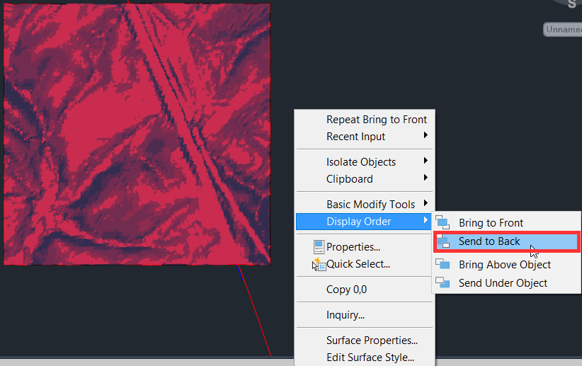
Figure 6.20 – Update Display Order of SRF - Existing Grade – FromSurveyPoints

As identified in Figure 6.21, there are several areas on our site where steeper slopes are present. It’s good to note these areas and ensure that as we progress through our design, we are able to stabilize these areas to withstand long-term weather events and support the construction of our design with minimal impact on the surrounding areas.

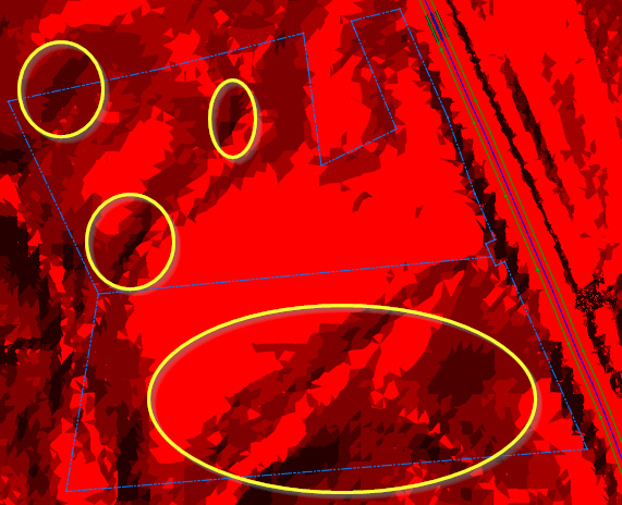
Figure 6.21 – Steep slopes within SRF - Existing Grade – FromSurveyPoints

Next, analysis that comes in handy as we prepare for our design is identifying elevation ranges, high and low spots on our site, and ridges and valleys to understand how and where our existing built environment is draining during storm events.

To perform this type of analysis, select the SRF - Existing Grade – FromSurveyPoints surface model again in the model space, right-click and select the Surface Properties option, just as we did when we started to perform our slope analysis previously.

Once the Surface Properties dialog box has appeared, we’ll switch back over to the Analysis tab and apply the following settings to begin our elevation analysis of our existing surface model (refer to Figure 6.22 for an image of settings):

• Analysis type: Elevations
• Legend: Elevations
• Create ranges by | Number of ranges: 8
• Click the down arrow icon below the Number of ranges field
• Adjust Minimum Elevation and Maximum Elevation in Range Details, as appropriate

Figure 6.22 – Surface Properties dialog box | Analysis tab – elevation analysis

Once we’re comfortable with our settings, we’ll then switch back over to the Information tab in the Surface Properties dialog box and apply the Elevation Banding (2D) surface style, as shown in Figure 6.23, and click on the OK button in the bottom right corner of the dialog box.

Figure 6.23 – Surface Properties dialog box | Information tab – Applying elevation display style

After clicking on the OK button to exit the Surface Properties dialog box, we can now see that the display of our surface has changed from displaying as Slope Banding (2D) to Elevation Banding (2D) across the entire surface model, as shown in Figure 6.24:

Figure 6.24 – Elevations and slope within SRF - Existing Grade – FromSurveyPoints

As identified in Figure 6.25, our existing site appears to be gradually sloping down toward the back of our site, away from York Highway. We can tell this by quickly identifying the high and low spots in our surface model when the Elevation Banding (2D) display style is applied. Furthermore, we can also identify how and where the existing site is draining water during storm events.

Figure 6.25 – SRF - Existing Grade – FromSurveyPoints drainage slopes

Taking this information into account, we’ll need to maintain similar drainage patterns as we progress through our design. By maintaining similar drainage patterns, we are minimizing disruption and any impact on surrounding properties and areas.

Furthermore, as we work through our design and think about the actual construction of it, we’ll need to apply similar tactics during the required construction phasing and staging and when designing and applying erosion control measures to our site.

Now that we have performed some initial investigation and interrogation of our existing surface model, giving us a decent idea of what we’re up against from a design standpoint, we can switch the SRF - Existing Grade – FromSurveyPoints surface model back to the Contours 2’ and 10’ (Background) display style.

We can do this by selecting our existing surface model again in the model space, right-clicking, and selecting the Surface Properties option one more time. Once the Surface Properties dialog box appears, we’ll go ahead and switch our display style from the Elevation Banding (2D) display style to the Contours 2’ and 10’ (Background) display style and click OK, as shown in Figure 6.26:

Figure 6.26 – Surface Properties dialog box – applying the Contours 2’ and 10’ (Background) display style

Following the steps outlined in Chapter 3, Sharing Data within Civil 3D, the last step we’ll take is to create a new data shortcut project, associate it with our current drawing, and then add our SRF - Existing Grade – FromSurveyPoints surface model so that we can later data reference for design purposes into our working models.

As shown in Figure 6.27, you’ll notice that when we create the data shortcut for our existing surface model, the subfolder entitled Existing Conditions that we created earlier in this chapter is automatically created as well.

As projects become more complicated and more team members are involved in project designs, this added level of organization in how we manage our modeled elements can be critical to keeping designs on track and under budget.

Figure 6.27 – Create the Data Shortcuts project and add the SRF - Existing Grade – FromSurveyPoints surface model

Summary

By now, we should have a pretty solid understanding of how we can best utilize survey point data to create, analyze, and manage our surface models. We’ve also begun to familiarize ourselves with the various styles associated with surfaces in particular and can begin thinking about the different ways we can apply each depending on the circumstances and intent.

In the next chapter, we’ll begin to explore alignments, including an overview of the various ways to create, manage, and apply all the styles associated with alignment geometry. We’ll also begin to understand how alignments are considered a foundational component that is common and integral to the majority of our designs.