CHAPTER 17
Macro and Managed Futures Funds
This first of five chapters on hedge fund strategies begins at, literally, the macro level. This chapter explores macro funds (i.e., global macro funds) and managed futures funds. Macro and managed futures strategies can differ substantially from other hedge fund strategies. Many investment strategies, especially in the arbitrage sector, focus on inefficiencies within markets at the security level. Macro and managed futures funds focus on the big picture, placing trades predominantly in futures, forward, and swap markets that attempt to benefit from anticipating price-level movements in major sectors or to take advantage of potential inefficiencies at sector and country levels. At the end of 2014, Hedge Fund Research (HFR) estimated that macro and managed futures funds managed $542.6 billion, which is 19.1% of the hedge fund universe.
17.1 Major Distinctions between Strategies
Macro and managed futures funds share many common features. They tend to have substantially greater liquidity and capacity and, when focused on exchange-traded futures markets, lower counterparty risks than hedge funds that follow other strategies. Capacity refers to the quantity of capital that a fund can deploy without substantial reduction in risk-adjusted performance. Counterparty risk is the uncertainty associated with the economic outcomes of one party to a contract due to potential failure of the other side of the contract to fulfill its obligations, presumably due to insolvency or illiquidity. This section focuses on the major distinctions within the category of macro and managed futures funds.
17.1.1 Discretionary versus Systematic Trading
Discretionary fund trading occurs when the decisions of the investment process are made according to the judgment of human traders. The trader may rely on computers for calculations and other data analysis, but in discretionary trading, the trader must do more than simply mechanically implement the instructions of a computer program. Despite the fact that computer programs are obviously written with human judgment, in discretionary trading there must be an ongoing and substantial component of human judgment.
Systematic fund trading, often referred to as black-box model trading because the details are hidden in complex software, occurs when the ongoing trading decisions of the investment process are automatically generated by computer programs. Although these computer programs are designed with human judgment, the ongoing application of the program does not involve substantial human judgment. Traders make decisions about when to use the program and may even adjust various parameters, including those that control the size and risk of positions. The key is that individual trades are not regularly subjected to human judgment before being implemented.
The concept of discretionary versus systematic trading applies to all investment processes, not just macro and managed futures funds. However, the distinction is especially relevant in discussing macro and managed futures funds. Global macro funds tend to use discretionary trading, and managed futures funds tend to use systematic trading. However, there are many exceptions, and some funds use discretionary trading for some of their trading activity and systematic trading for their other trading activity.
17.1.2 Fundamental and Technical Analysis
Trading strategies are based on analysis of information. A major distinction is whether the investment strategy analyzes information with fundamental analysis, technical analysis, or both. Briefly, technical analysis relies on data from trading activity, including past prices and volume data. Fundamental analysis uses underlying financial and economic information to ascertain intrinsic values based on economic modeling. Trading decisions can be based purely on technical or fundamental analysis or on a combination of the two. For example, some investment processes rely on fundamental analysis to determine potential long and short positions and on technical analysis to determine the timing of entering and exiting those positions.
Technical analysis focuses on price movements due to trading activity or other information revealed by trading activity to predict future price movements. Typically, technical analysis quantitatively analyzes the price and volume history of one or more securities with the goal of identifying and exploiting price patterns or tendencies.
One motivation for using technical analysis is based on the idea that prices already incorporate some economic information, but price patterns may be identified that could be exploited for profit opportunities. The underlying assumption is that prices may not instantaneously and completely reflect all available information (i.e., prices may be slow to react to new information). For instance, if there is asynchronous global economic growth, one might forecast exploitable price movements as some local markets (e.g., in country-specific equity indices) react on a delayed basis to information already reflected in larger and more efficient markets. A common strategy in macro and managed futures funds is to attempt to exploit currency exchange rate movements, such as trends resulting from announced government intervention in foreign exchange markets. The key to this technical trading is the assumption that although prices are predominantly based on underlying economic information, analysis of trading activity can reveal consistent patterns of how prices respond to new information.
A second motivation to pursuing strategies based on technical analysis is a belief that market prices are substantially determined by trading activity that is unrelated to a rational analysis of underlying economic information. These technical strategies attempt to identify price patterns generated by trading activity and to identify those patterns on a timely basis. An example would be a prediction that an index is not likely to pass through a particular level as it approaches that level (e.g., an index nearing a round number such as 1,000), but if that level is breached, then the price is likely to continue moving in the same direction.
Fundamental analysis attempts to determine the value of a security or some other important variable through an understanding of the underlying economic factors. Fundamental analysis can be performed at a macro level using economy-wide information, such as economic growth rates, inflation rates, unemployment rates, and data on commodity supply and demand. It can also be performed at the micro level using firm-specific data, such as revenues, expenses, earnings, and dividends, or security-specific information. Fundamental analysis often focuses on predicting price changes to securities based on current and anticipated changes in underlying economic factors. Underlying economic factors can include (1) market or economy-wide factors, such as changes to monetary or fiscal policies; (2) industry-wide factors, such as changes in relevant commodity prices or consumer preferences; and (3) firm-specific factors, such as product innovations, product failures, labor strikes, or accidents.
Fundamental analysis and technical analysis are used throughout alternative investments strategies, but the distinction in macro and managed futures funds is especially interesting. As in the case of distinguishing between discretionary and systematic trading, some funds focus on strategies using fundamental analysis, some focus on strategies using technical analysis, and some have a mix. However, systematic trading strategies tend to be built around technical analysis.
17.1.3 Organization of the Chapter
There are sufficient similarities between macro funds and managed futures funds to combine in this chapter. Global macro funds are more likely to be discretionary and emphasize fundamental analysis, whereas managed futures tend to be more systematic and emphasize technical analysis. So although exceptions are frequent, the remainder of this chapter begins with a section on global macro funds to discuss the use of discretionary trading and strategies based on fundamental analysis. Then, the section on managed futures funds discusses futures contracts, systematic trading, and technical analysis.
17.2 Global Macro
Most macro funds employ discretionary trading and are often concentrated in specific markets or themes. As their name implies, global macro hedge funds take a macroeconomic approach on a global basis in their investment strategy. These are top-down managers who invest opportunistically across national borders, financial markets, currencies, and commodities. They take large positions that are either long or short, depending on the hedge fund manager's forecast of changes in equity prices, interest rates, currencies, monetary policies, and macroeconomic variables such as inflation, unemployment, and trade balances.
Global macro funds have the broadest investment universe: They are not limited by market segment, industry sector, geographic region, financial market, or currency, and therefore tend to offer high diversification. Macro funds tend to have low correlation to stock and bond investments, as well as to other types of hedge funds. Given their broad mandate, the returns earned by macro managers may also have relatively low correlation to other macro funds.
The ability to invest widely across currencies, commodities, financial markets, geographic borders, and time zones is a double-edged sword. On the one hand, this mandate allows global macro funds the widest universe in which to implement their strategies. On the other hand, it lacks a predetermined focus. As more institutional investors have moved into the hedge fund marketplace, they are demanding fund managers who offer greater investment focus rather than investing with managers who have free rein.
17.2.1 Illustrations of Global Macro Fund Investing
Global macro funds tend to have large amounts of investor capital. In addition, they may apply leverage to increase the size of their macro bets. As a result, global macro hedge funds tend to receive the greatest attention and publicity in the financial markets. Although macro managers have broad latitude in their trades, examples of trading strategies that are common or classic across managers are discussed here, to illustrate the essence of global macro fund investing.
The first example deals with potential profit opportunities when national governments impose fixed or managed exchange rates. Macro managers often seek to invest in markets that they perceive to be out of equilibrium or that exhibit a risk-reward trade-off skewed in the manager's favor. High levels of competition tend to drive market prices to approximate their informationally efficient values. However, actions by powerful national governments can, at least temporarily, cause market prices to diverge substantially from their expected long-run values in the absence of government actions. Perhaps the best example of these types of trades can be found in countries where the government has mandated fixed or managed currency rates between its currency and the currency of one or more other nations. Managers of macro funds monitor these currencies and estimate the likelihood of a currency revaluation or devaluation to a price other than the official rate.
Fund manager George Soros speculated famously in currency markets in the 1990s through the Quantum Fund. Soros made substantial gains in 1992 by successfully wagering that the British pound would devalue. In the days before the euro, the British pound (GBP) was a member of the European Exchange Rate Mechanism (ERM), which sought to keep currencies within a specified range of values relative to other European currencies. Specifically, the GBP was not allowed to deviate by more than 6% relative to its official rate, stated in terms of German deutsche marks (DM). When the pound reached the limit of 6% below the target rate, the British government would intervene to raise the value of the GBP relative to the DM. For the GBP, this scheme fell apart in September 1992. Hedge funds and other market participants were short selling the GBP, betting that the British government would stop purchasing the GBP in order to defend the ERM rate and system. Finally, the GBP moved to a floating rate and exited the ERM. The GBP suffered an overnight loss of 4% and fell 25% versus the U.S. dollar by the end of 1992. Those who were short GBP against DM were able to book a large and swift profit as the market forced the GBP to trade at a rate more reflective of the fundamentals. At the time, Germany had stronger monetary and fiscal policy fundamentals.
Soros was accused of contributing to the Asian contagion in the fall of 1997, when Thailand devalued its currency, the baht, triggering a domino effect in currency movements throughout Southeast Asia. In this case, Thailand, Malaysia, and Indonesia had currency rates that were pegged relative to a basket of currencies, with a heavy weighting to the U.S. dollar. Each country had high interest rates, large external debt, and large current account deficits, in which the value of imports exceeded the value of exports. Soros and other market participants increasingly short sold these currencies at the government-supported fixed exchange rates, and the respective governments seemed to be the only buyers. Eventually, each government exhausted its official reserves and was forced to stop the defense of its currency. Once the governments stopped buying their currency at the official rate, each currency moved to a freely floating value. Within a short time, the Thai baht and other Asian currencies declined by 40% to 70%.
Markets for sovereign bonds may also present global macro funds with potential trade and profit opportunities. In addition to attempting to control currency rates, national governments exert enormous influence on the interest rates of their bonds, which are known as sovereign bonds. Global macro hedge fund managers often speculate on sovereign bond prices. Between 1994 and 1998, a bullish bet was to take large positions on new entrants into the euro currency. The sovereign bonds of Portugal, Italy, Greece, and Spain—the countries that joined the euro currency in 2001—were extraordinarily profitable investments as the countries prepared to enter the economic union. As with all countries seeking to enter the union, these nations were required to meet the terms of the Maastricht Treaty, which required annual government budget deficits below 3% of GDP, total national debt below 60% of GDP, an inflation rate no higher than 1.5% above the strongest member countries, and long-term interest rates within 2% of the current members of the union.
As indications of the profits earned by funds establishing long positions in the debt and equity of countries entering the economic union, note that Greek sovereign bonds denominated in drachmas yielded 25% in 1994 and declined to 11% by 1998, whereas the Greek stock market increased by 130% between 1998 and 1999. More recently, some funds have profited from shorting sovereign debt.
Macro managers are expert at understanding the impact of central bank intervention in the markets. A recent example is the election of Shinzo Abe as the prime minister of Japan. His 2012 campaign focused on economic reform, seeking to restore inflation and economic growth after two decades of malaise. Abe's plan, now deemed “Abenomics,” had three arrows: aggressive monetary easing, large public investments, and structural reforms. In just over one year, the monetary supply doubled, which led to a quick increase in the Nikkei index of over 50% and a decline in the yen against many world currencies of approximately 20%. Macro managers with long stock and short yen positions made quick and substantial profits by buying into the short-term stimulus measures implemented by Abe shortly after his election. As the value of the yen declines, exports become more competitive and profitable. The goal is for these increased profits of large exporting firms to result in increased investment, productivity, employment, and wages. Ideally, these higher incomes would lead to increased domestic spending and consumption.
Macro managers, though, need to separate the short-term stimulus from the long-term effects and decide whether Abenomics will continue its effect on asset and currency prices or the long-term decline in the economy is more difficult to reverse. In the first half of 2014, the Nikkei declined by over 7% while the yen strengthened by an even greater amount.
Fighting against Abenomics are demographics, a consumption tax increase, and the delay of a decline in corporate tax rates from 35% to a desired 29%. Demographics are difficult, as the population of 127 million is expected to decline to less than 87 million by 2060, according to the National Institute of Population and Social Security Research. As the number of retirees increases and the number of births declines, old age benefits deplete government budgets faster than young entrants can increase the productive workforce and the resulting income tax payments. When sales taxes were increased from 3% to 5% in 1997, a multiyear recession ensued. This consumption tax increased to 8% in 2014 and is expected to reach 10% in 2015. These recent tax increases offset the optimism that higher stock prices and easing monetary policy are meant to provide. While exports have increased, domestic job growth and consumer demand remain weak, even in the face of import price inflation.
Thematic investing is a trading strategy that is not based on a particular instrument or market; rather, it is based on secular and long-term changes in some fundamental economic variables or relationships—for example, trends in population, the need for alternative sources of energy, or changes in a particular region of the world economy. The last type is exemplified by the rise of China. Investors who believe that Chinese GDP growth will remain strong have a wide variety of trading ideas, many of them outside the Chinese markets. One such view might be the decline of the developed markets of the United States and Europe as they continue to deal with large trade and budget deficits. China's rise may have benefits for other Asian countries, including Japan, India, and South Korea. The strength of the Chinese economy may cause even the Chinese to outsource, which could lead to economic growth and additional wage income in less developed Asian countries, such as Vietnam. The power of China is, perhaps, most clearly seen in making the bullish case for commodity prices. China's rise has accounted for a substantial portion of the world's increased demand for a number of commodities. As China continues to urbanize and industrialize, building new roads, cities, workplaces, and consumer goods will continue to stoke the demand for commodities. Of course, China's growth could falter, much as Japan faltered economically after the 1980s. Savvy global macro managers who are able to better predict these major global economic themes may use bets in commodity markets and other markets to attempt to generate superior returns.
These examples of common global macro investing illustrate the role of macroeconomics in the implementation of the strategy. Many of the hedge fund strategies discussed in the remaining chapters of Part 3 are implemented through an understanding of individual firms, individual securities, and market microstructure. Market microstructure is the study of how transactions take place, including the costs involved and the behavior of bid and ask prices. But each of the examples of global macro investing just discussed is more concerned with the economic workings of economy-wide or even global markets, institutions, and forces. The illustrations involved exchange rates, interest rates, inflation rates, country economic growth rates, regional growth rates, and so forth.
Success in global macro investing requires superior skills in forecasting changes at the macroeconomic level. The necessary macroeconomic analysis can be performed qualitatively or quantitatively. Quantitative macroeconomic models can be empirical models of how markets have behaved (i.e., positive models) or theoretical models of how they ought to behave (i.e., normative models). The models vary in size and sophistication. However, the importance of experience, intuition, and data gathering should not be underestimated.
17.2.2 Three Primary Risks of Macro Investing
Macro funds often have higher risk exposures than most other strategies to market risk, event risk, and leverage risk.
Market risk refers to exposure to directional moves in general market price levels. Macro funds typically do not focus on equity markets, as equities can be highly influenced by microeconomic factors, such as company-specific events. However, macro funds can take substantial and concentrated risks in currency, commodity, and sovereign debt markets, especially when it is believed that changes in governmental policies will lead to large moves in the underlying markets.
Event risk refers to sudden and unexpected changes in market conditions resulting from a specific event (e.g., Lehman Brothers bankruptcy). Macro funds attempt to benefit from particular events. They seek profits from large market dislocations, especially those involving governmental financial policies. However, because macro funds seek out situations of event risk at the macroeconomic level, these funds can have substantial changes in value over short periods of time.
Leverage refers to the use of financing to acquire and maintain market positions larger than the assets under management (AUM) of the fund. Leverage is typically established through borrowing or derivatives positions and poses risks. Funds with leverage may be forced to deploy additional capital if they experience losses, and if they are unable to do so, they may be forced to liquidate positions at the least opportune time. Magnifying the risk of their concentrated positions in markets with substantial event risks, many macro funds use futures, swap, and forward markets to increase the leverage of the fund. While gains can be substantial, leverage can also lead to dramatic losses. Leverage in these derivatives markets, though, is less problematic than leverage in single securities sourced through prime brokers, as derivatives markets are less likely to require large changes in margin without notice.
17.3 Returns of Macro Investing
Exhibit 17.1 provides an analysis of global macro fund monthly returns, as indicated by the Credit Suisse Global Macro Index (CSGMI) alongside the HFRI Macro Index, following the standardized framework detailed in the appendix. The HFRI Macro Index contains a variety of strategies, including macro discretionary thematic, systematic diversified, multistrategy, and several commodity strategies. Exhibit 17.1a indicates the high mean returns, low volatility, and excellent risk-adjusted performance of global macro funds from January 2000 through December 2014. The Sharpe ratio of the CSGMI is substantially higher than the Sharpe ratios of global stocks, global bonds, U.S. high-yield bonds, or commodities. The minimum monthly returns and maximum drawdowns also support the superior historical performance of both indices over the 15-year interval.
Exhibit 17.1A Statistical Summary of Returns
| Credit Suisse | HFRI Macro | World | Global | U.S. High- | ||
| Index (Jan. 2000−Dec. 2014) | Global Macro | (Total) | Equities | Bonds | Yield | Commodities |
| Annualized Arithmetic Mean | 9.6%** | 5.7%** | 4.4%** | 5.7%** | 7.7%** | 3.8%** |
| Annualized Standard Deviation | 5.5% | 5.2% | 15.8% | 5.9% | 10.0% | 23.3% |
| Annualized Semistandard Deviation | 4.5% | 2.9% | 12.0% | 3.6% | 9.0% | 16.8% |
| Skewness | –1.0** | 0.3 | –0.7** | 0.1 | –1.0** | –0.5** |
| Kurtosis | 4.1** | 0.4 | 1.5** | 0.6* | 7.7** | 1.3** |
| Sharpe Ratio | 1.35 | 0.67 | 0.14 | 0.60 | 0.56 | 0.07 |
| Sortino Ratio | 1.63 | 1.19 | 0.18 | 0.97 | 0.62 | 0.10 |
| Annualized Geometric Mean | 9.4% | 5.5% | 3.1% | 5.5% | 7.2% | 1.1% |
| Annualized Standard Deviation (Autocorrelation Adjusted) | 6.4% | 5.4% | 18.3% | 6.2% | 13.3% | 27.9% |
| Maximum | 5.0% | 5.7% | 11.2% | 6.6% | 12.1% | 19.7% |
| Minimum | –6.6% | –3.7% | –19.0% | –3.9% | –15.9% | –28.2% |
| Autocorrelation | 16.2%** | 3.2% | 16.0%** | 6.1% | 30.7%** | 19.4%** |
| Max Drawdown | –14.9% | –8.0% | –54.0% | –9.4% | –33.3% | –69.4% |
* = Significant at 90% confidence.
** = Significant at 95% confidence.
Exhibit 17.1b illustrates the relatively high return and low risk of the CSGMI relative to global equities through a cumulative wealth chart. The CGSMI was relatively unscathed by the financial crisis that began in 2007 relative to equities, yet was able to generate substantial growth prior to the crisis.

Exhibit 17.1B Cumulative Wealth
Exhibit 17.1c provides mixed correlations of both macro indices to major market indices. Note that the HFRI Macro Index was statistically uncorrelated to changes in the credit spread.
Exhibit 17.1C Betas and Correlations
| Index (Jan. 2000−Dec. 2014) | World | Global | U.S. High- | Annualized | ||
| Multivariate Betas | Equities | Bonds | Yield | Commodities | Estimated α | R2 |
| Credit Suisse Global Macro | –0.01 | 0.29** | 0.07 | 0.06** | 5.88%** | 0.24** |
| HFRI Macro (Total) | 0.07** | 0.27** | –0.06 | 0.05** | 2.66%** | 0.23** |
| World | Global | U.S. High- | %Δ Credit | |||
| Univariate Betas | Equities | Bonds | Yield | Commodities | Spread | %Δ VIX |
| Credit Suisse Global Macro | 0.08** | 0.37** | 0.15** | 0.08** | –0.02* | –0.02** |
| HFRI Macro (Total) | 0.09** | 0.33** | 0.08** | 0.08** | –0.01 | –0.02** |
| World | Global | U.S. High- | %Δ Credit | |||
| Correlations | Equities | Bonds | Yield | Commodities | Spread | %Δ VIX |
| Credit Suisse Global Macro | 0.25** | 0.39** | 0.27** | 0.34** | –0.14** | –0.23** |
| HFRI Macro (Total) | 0.28** | 0.37** | 0.16** | 0.34** | –0.06 | –0.20** |
* = Significant at 90% confidence.
** = Significant at 95% confidence.
Finally, Exhibit 17.1d indicates modest correlation between the CSGMI strategy and world equities via a scatter plot. Note that the very worst months for world equities correspond with the worst months for the cross-sectionally averaged returns of the CSGMI. However, some very strong months for the CSGMI correspond to down months for equities, as shown in the lower right quadrant.

Exhibit 17.1D Scatter Plot of Returns
17.4 Managed Futures
Futures contracts emerged in the agricultural markets of the 1800s as cost-effective vehicles for the transfer and management of the risk related to uncertain crop prices. The history of managed futures products goes back to the middle of the 1900s. The first public futures fund began trading in 1948 and was active until the 1960s. That fund was established before financial futures contracts were invented, and it consequently traded primarily in agricultural commodity futures contracts. The success of that fund spawned other managed futures vehicles, and a new industry was born. Financial futures contracts emerged in the 1970s and eventually offered opportunities for market participants to transfer and manage a variety of financial risks, including equity market risk, interest rate risk, exchange rate risk, and credit risk. With the advent and rapid growth of financial futures contracts, more and more managed futures trading funds and strategies were born.
The term managed futures refers to the active trading of futures and forward contracts on physical commodities, financial assets, and exchange rates. The purpose of the managed futures industry is to enable investors to receive the risk and return of active management within the futures market while enhancing returns and diversification.
The managed futures industry provides a skill-based style of investing. Investment managers attempt to use their special knowledge and insight to establish and manage long and short positions in futures and forward contracts for the purpose of generating consistent, positive returns. These futures managers tend to argue that their superior skill is the key ingredient in generating profitable returns from the futures markets.
Managed futures strategies tend to be based on systematic trading more than discretionary trading. Further, futures managers tend to use more technical analysis, as opposed to trading based on fundamental analysis. This section on managed futures takes a detailed look at systematic trading and technical analysis. The section begins, however, with an overview of futures contracts and futures markets.
17.4.1 Futures Contracts and Futures Markets
Chapters 6, 11, and 12 provide detailed foundational material on the pricing of futures contracts and forward contracts. For the purposes of this chapter, it suffices to know that futures and forward contracts are similar and can be cost-effective means of establishing positions with risk exposures that very closely approximate those that can be established in the cash market. For example, a market participant may wish to speculate that a particular price, such as the price of corn, gold, a stock index, or a Japanese government bond, is likely to rise. The speculator could buy those assets in the cash market, store them, and then sell them to close the trade. However, cash positions can have numerous disadvantages, such as storage costs, financing costs, higher transaction costs, inconvenience, and restrictions on short selling. Market participants with short-term trading horizons often prefer futures and forward contracts. Futures and forward contracts usually offer lower transaction costs, higher liquidity, more observable pricing, and more flexibility to short sell.
17.4.2 Regulation, Background, and Organizational Structures
Until the early 1970s, the managed futures industry was largely unregulated. Anyone could advise an investor regarding commodity futures investing or form a fund for the purpose of investing in the futures markets. Recognizing the growth of this industry, the industry's potential impacts on an economy, and the lack of regulation associated with the industry, regulatory authorities have been established for managed futures funds, futures contracts, and, to a lesser extent, forward contracts.
For example, in the United States in 1974, Congress enacted the Commodity Exchange Act (CEA) and created the Commodity Futures Trading Commission (CFTC). Under the CEA, Congress first defined the terms commodity pool operator (CPO) and commodity trading adviser (CTA). In addition, Congress established standards for financial reporting, offering memorandum disclosure and bookkeeping. Congress required CTAs and CPOs to register with the CFTC. Last, Congress required CTAs and CPOs to undergo periodic educational training in cooperation with the National Futures Association (NFA), the designated self-regulatory organization for the managed futures industry.
Commodity trading advisers may invest in both exchange-traded futures contracts and forward contracts. The economic structure of forward contracts is highly similar to that of futures contracts, with the most major difference being that futures contracts are exchange-traded while forward contracts are usually traded over the counter. Forward contracts are private agreements. Therefore, they can have terms that vary considerably from the standard terms of exchange-listed futures contracts. Forward contracts accomplish virtually the same economic goal as a futures contract but with the flexibility of custom-tailored terms. However, futures contracts provide substantial protection against counterparty risk as a result of being backed by the exchange's clearinghouse, whereas forward contracts are exposed to full counterparty risk. In the remainder of this chapter, both types of contracts are referred to as futures contracts.
There are three ways to access the skill-based investing of the managed futures industry:
- Public commodity pools
- Private commodity pools
- Individually managed accounts
Commodity pools are investment funds that combine the money of several investors for the purpose of investing in the futures markets. Public commodity pools are open to the general public for investing in much the same way that a mutual fund sells its shares to the public. In the United States, public commodity pools must file a registration statement with the SEC (Securities and Exchange Commission) before distributing shares in the pool to investors. An advantage of public commodity pools is the low minimum investment and the high liquidity that they provide for investors, allowing them to withdraw their investments with relatively short notice (compared to other hedge fund strategies).
Private commodity pools are funds that invest in the futures markets and are sold privately to high-net-worth investors and institutional investors. They are similar in structure to hedge funds and are increasingly considered a subset of the hedge fund marketplace. Commodity pools are managed by a general partner. In the United States, the general partner for the pool must typically register with the CFTC and the NFA as a CPO. However, there are exceptions to the general rule. Private commodity pools are organized privately to avoid lengthy or burdensome initial regulatory requirements, such as registration with the SEC in the United States, and to avoid ongoing reporting requirements, such as those of the CFTC in the United States. Otherwise, their investment objective is the same as that of a public commodity pool. Advantages of private commodity pools are usually lower fees and greater flexibility to implement investment strategies.
The CPOs for either public or private pools typically hire one or more CTAs to manage the money deposited with the pool. Commodity trading advisers (CTAs) are professional money managers who specialize in the futures markets. Some CPOs act as a fund of funds, diversifying investments across a number of CTA products. Like CPOs, CTAs in the United States must register with the CFTC and the NFA before managing money for a commodity pool. In some cases, a managed futures investment manager is registered as both a CPO and a CTA. In this case, the general partner for a commodity pool may also act as its investment adviser.
In addition, wealthy investors and institutional investors may use a managed account. A managed account (or separately managed account) is created when money is placed directly with a CTA in an individual account rather than being pooled with other investors. When large enough to be cost-effective, managed accounts offer numerous advantages over pooled arrangements. These separate accounts have the advantage of representing narrowly defined and specific investment objectives tailored to the investor's preferences. With a managed account, the investor retains custody of the assets with the investor's regular broker and only needs to allow the CPO or CTA to exert trading authority in the account. Other advantages to the investor include transparency and control, which allow the investor to see all of the trading activity, as well as the ability to increase or decrease the leverage applied.
Like hedge funds, CTAs and CPOs charge management fees and incentive fees. The standard hedge fund fees of 2 and 20 (2% management fee and 20% incentive fee) are equally applicable to the managed futures industry, although management fees can range from 0% to 3%, and incentive fees can range from 10% to 35%.
17.5 Systematic Trading
Systematic trading is usually quantitative in nature and often referred to as computer-based, model-based, or black-box trading. Systematic trading in this context refers to the automation of the investment process, not to systematic risk. Systematic trading models apply a fixed set of trading rules in determining when to enter and exit positions. Deviation from the system's rules is generally not permitted.
17.5.1 Derivation of Systematic Trading Rules
Systematic trading rules are generally derived from backtests. In the context of systematic trading rules, a backtest is an identification of a price or return pattern that appears to persist, as located and verified through a quantitative analysis of historical prices. Trading systems are generally based on the expectation that historical price patterns will recur in the future. However, many trading systems that appear to perform well using backtested data end up performing poorly when they are implemented in real time. Statistics show that when many analysts search through many data sets with many hypothetical trading systems, very many trading systems appear ex post to be profitable but in fact are generated purely by randomness or by market regimes that no longer exist. Being able to avoid data dredging and false identification of attractive trading rules is the key to successful backtesting.
Backtests should also have reasonable estimates for transaction costs and slippage. Slippage is the unfavorable difference between assumed entry and exit prices and the entry and exit prices experienced in practice. Thus, an analyst observing a long history of daily closing prices should assume that an actual trading strategy is likely to generate less favorable price executions due to the tendency of buy orders to push prices up, or be executed at an offer price, and of sell orders to push prices down, or be executed at a bid price. Care should also be taken to ensure that reported prices on which backtests are performed are executable prices rather than stale prices or published indications of prices, and that they are free from large errors.
Systematic traders rarely employ only a single trading system with a single security. Managers who have success with one trading system in one market typically search for other markets in which that trading system, or a modified version of it, can be successfully applied. Over time, managers may modify their trading systems, develop new ones, and abandon others.
17.5.2 Three Questions in Evaluating a Systematic Trading System
There are three useful questions to ask when evaluating an individual trading strategy:
- What is the trading system, and how was it developed? Here, one is looking to understand the broad underlying trading approach (e.g., trend following versus countertrend) and specific characteristics of the strategy itself. It is also important to understand the research methods used to identify and develop the trading strategy to avoid strategies based on spurious results from data dredging. Poor research methods can lead to overfitting of historical data, such that a historical price series may appear to have a recurring pattern yet be in fact random.
- Why and when does the trading system work, and why and when might it not work? It is important to understand the underlying hypothesis of a specific trading strategy. If the trading system is making money for its investors, from where or from whom is that money coming? Such understanding is important in and of itself but is also critical in identifying market conditions that are likely to be supportive of the strategy (e.g., trend accompanied by low volatility). Although it may be difficult to forecast market conditions, understanding what impact various market conditions are likely to have on the strategy's performance is important in interpreting the potential success or failure of a strategy over time.
- How is the trading system implemented? Many operational factors contribute to a successful systematic trading strategy, including selection of data sources, determination of periodicity of data, establishment of protocols to clean the data, processing of the data into a trading signal, placement of trades, record keeping, and broker reconciliation.
The key to systematic trading systems is to differentiate spurious results from results that will persist. Similarly, analysts seek to ascertain whether trading systems that were successful in the past but have stopped working recently will perform poorly on a temporary basis or on a permanent basis. In other words, at what point should a trading system be abandoned or modified if the system worked very well in the past but has generated poor results recently?
17.5.3 Validation and Potential Degradation of Systematic Trading Rules
Systematic managed futures strategies rely on quantitative research methods that backtest trading rules using historical price data. Validation of a trading rule refers to the use of new data or new methodologies to test a trading rule developed on another set of data or with another methodology. For example, a trading rule developed analyzing data during five calendar years should be tested first in subperiods of those five years to see if the results are robust across data sets and sub-intervals. Robustness refers to the reliability with which a model or system developed for a particular application or with a particular data set can be successfully extended into other applications or data sets.
Most important, validation of the trading rule should be performed with out-of-sample data. Out-of-sample data are observations that were not directly used to develop a trading rule or even indirectly used as a basis for knowledge in the research. For example, the trading rule should be validated on the most recent data, which, of course, should not have been used explicitly or implicitly in the model's development. In-sample data are those observations directly used in the backtesting process. Out-of-sample data consist of more recent data than were used in the backtest. Out-of-sample data should be used to test the profitability of a trading strategy beyond the period covered by the backtest. The goal is to avoid data dredging and to ensure that a trading rule generates persistent performance.
Further, it is vital to know how many trading rules were tested, how many were subjected to validation, and how many were rejected in the validation process. If 20 trading rules (e.g., one model with 20 different parameter values) are subjected to validation, one of them on average will survive a validation process with a confidence interval of 95%, even if none of the rules truly offers value-added properties. More to the point, if several analysts test hundreds of strategies (e.g., hundreds of parameter values) on numerous data sets (e.g., securities), then numerous trading strategies will survive the validation process unless the validation process is carefully designed to incorporate into its statistical approach the total number of tests performed.
Trading rules typically evolve over time as analysts try to optimize profitability. Analysts perform ongoing research to estimate and refine trading parameters, add new trading parameters, and drop old trading parameters. Markets also typically evolve over time. A once-profitable price pattern that becomes identified and exploited by numerous CTAs eventually ceases to exist or substantially changes. Therefore, a trading model or trading strategy that has been successful over the past 10 years often experiences degradation and is not profitable over the next 10 years. In this context, degradation is the tendency and process through time by which a trading rule or trading system declines in effectiveness. The key is to differentiate between (1) trading rules that are being changed to better identify true price patterns, and (2) trading rules that are data dredging for a pattern that no longer exists. Both an effective trading system and a fully degraded trading system experience episodes of high returns and episodes of poor returns due to randomness. Identifying which systems remain effective and which have degraded requires careful statistical analysis as well as informed qualitative analysis.
17.6 Systematic Trading Strategies
Systematic trading strategies are generally categorized into three groups: trend-following, non-trend-following, and relative value.
17.6.1 Trend-Following Strategies
Trend-following strategies are designed to identify and take advantage of momentum in price direction (i.e., trends in prices). Momentum is the extent to which a movement in a security price tends to be followed by subsequent movements of the same security price in the same direction. Trend-following strategies use recent price moves over some specific time period (e.g., ranging from a few minutes to several hundred days) to identify a price trend. The goal is to establish long positions in assets experiencing an upward trend, establish short positions in assets experiencing a downward trend, and avoid positions in assets not experiencing a trend.
Mean-reverting refers to the situation in which returns show negative autocorrelation—the opposite tendency of momentum or trending. An asset that consistently tends to return toward its previous price level after a move in one direction is typically said to be mean-reverting or to exhibit mean reversion. Mean reversion is the extent to which an asset's price moves toward the average of its recent price levels. Trending markets exhibit returns with positive autocorrelation. A price series with changes in its prices that are independent from current and past prices is a random walk. Therefore, momentum and mean reversion are properties that are not consistently displayed by prices that follow a random walk.
One of the most popular classes of trend-following strategies uses moving averages to signal trades. A moving average is a series of averages that is recalculated through time based on a window of observations. The most basic approach uses a simple moving average, a simple arithmetic average of previous prices. More sophisticated averaging techniques place a greater weight on more recent prices. The formula for calculating a simple moving average, SMAt(n), is shown in Equation 17.1, where t is the current time period and n is the number of time periods used in the computation:
The window of observations is composed of a fixed number of lagged prices. For example, a current 10-day moving average price (day 0) is formed using the 10 prices corresponding to the 10 days immediately preceding the current price (days –1 to –10). Yesterday's (day –1) 10-day moving average would be composed of the prices corresponding to the 10 days prior to that day (days –2 to –11). Exhibit 17.2 summarizes the process along with the classic trading signals based on a simple trend-following rule.
Exhibit 17.2 Simple Moving Average Summary
| Description: | In a simple moving average, the daily prices are equally weighted. As each new price observation is added to the series, the oldest observation falls away, creating a window of averaged prices that is often charted. |
| Signals: | Enter long if current price Pt > SMAt(n)
Enter short if current price Pt < SMAt(n) |
Like the underlying market itself, the moving average price changes every day, but the moving average changes value in a lagged and muted fashion relative to the current price. The shorter the time period used to calculate the moving average, the more quickly the average will respond to changes in the level of more current prices, the more volatile the average will be, and, generally, the more times the current price will cross over the moving average price (i.e., the more trading signals will be generated).
Numerous variations of moving average computations exist:
- The number of periods (and the length of the time period) used in the moving average, n, can vary (e.g., 10-day versus 30-day versus 60-minute).
- The entry and exit levels can be a percentage of the moving average (e.g., enter when the current price exceeds the moving average by 1%).
- An unequally weighted moving average can be calculated, using an averaging process that weights recent prices more heavily than older prices.
There are trading signals other than the comparison of the current price to a single moving average. For example, trading signals to establish long positions may be identified as follows:
- When the current price exceeds two or more moving averages (e.g., both the 10-day and the 30-day moving averages)
- When a shorter-term moving average crosses up and over a longer-term moving average
- When moving averages align upward (i.e., are all in the same direction, with the shorter moving averages exceeding the longer moving averages)
The three computational variations taken together with the various signal identification rules generate an astounding number of possible strategies. The abundance of potential strategies leads to the potential problem of data dredging, in which so many potential strategies can be tested that strategies will be identified that satisfy empirical tests with high levels of statistical confidence even when true patterns do not exist.
There are two major approaches to weighting more recent prices more heavily than older prices: weighted moving averages and exponential moving averages.
17.6.2 Weighted Moving Averages and Exponential Moving Averages
Although simple moving averages are the most commonly used measures, weighted and exponential moving averages are also used and have the potential advantage of assigning larger weights to the most recent prices.
A weighted moving average is usually formed as an unequal average, with weights arithmetically declining from most recent to most distant prices. To illustrate, the length of the averaging interval (i.e., the number of observations used in the computation of each average) is denoted as n. The oldest price is multiplied by 1,
the second oldest price is multiplied by 2, and so forth, until the most recent price is multiplied by n. Each product is then divided by the sum of the digits. The n-period weighted moving average, WMAt(n), is shown in Equation 17.2:

In the case of n = 4, the sum of the labels, N, is 10 (the sum of 1 through 4). The most recent previous price (Pt–1) is weighted 40% (4/10), the second most recent price is weighted 30% (3/10), and so forth, until the oldest price is weighted only 10% (1/10). Note that the weights decline arithmetically: 40%, 30%, 20%, and 10%.
The exponential moving average is a geometrically declining moving average based on a weighted parameter, λ, with 0 < λ < 1. The most recent observation is weighted through multiplication by the weighted parameter, λ. All other previous observations are weighted by λ (1 – λ)n, in which n is the length of the time lag. For example, with λ = 0.4, the most recent observation is multiplied by 0.4. The second and third most recent observations are weighted by λ (1 – λ)1 and λ (1 – λ)2 (0.24 and 0.144), respectively. The formula for the exponential moving average at time t, EMAt(λ), is given next in an expanded form (Equation 17.3a) and a reduced form (Equation 17.3b):
Equation 17.3a illustrates the intuition of the exponential moving average. The most recent price receives the weighted parameter, λ. The terms after the first term are multiplied both by λ and by (1 – λ)n. Since (1 – λ) is less than 1, the weight assigned to each previous price declines as the price becomes more distant. The problem with Equation 17.3a is that to compute EMAt(λ) using that equation requires input of the entire history of the price series.
Equation 17.3b denotes how the exponential moving average is calculated in practice. In this view, today's exponential moving average is a weighted average of the current price and yesterday's exponential moving average. Inspection of either equation reveals that the formula requires an infinitely long history of previous prices. Therefore, in practice, computation is performed by seeding some initial value to EMAt–1. Once an initial approximation is set for a previous value of the exponential moving average, all subsequent exponential moving averages are simply computed as the sum of λ times the most recent price (1 – λ) times the most recent exponential moving average.
17.6.3 An Illustration of a System Using Two Moving Averages
Exhibit 17.3 illustrates a strategy employing two moving averages to generate trading signals. In the example, the strategy uses a 10-day and a 45-day moving average as the shorter-term and the longer-term indicators, respectively. The first signal in the example (denoted with a vertical line) is a sell signal (i.e., a signal to establish a short position), because the 10-day moving average line (the shorter average) crossed below the 45-day moving average line (the longer average). Some days later, a signal to establish a long position emerged when the 10-day moving average line crossed above the 45-day moving average line.
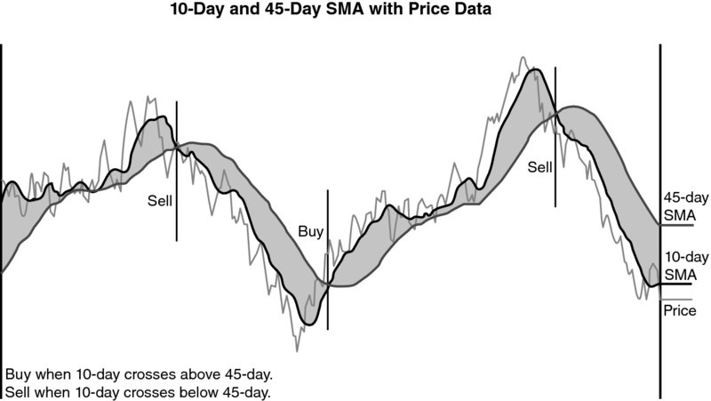
Exhibit 17.3 Example with Two Simple Moving Averages
Exhibit 17.3 appears to illustrate a highly successful trading period with two sell signals at prices much higher than the buy signal. Trend-following strategies perform well when there is an extended move in the price from one level to another, and tend to be more powerful when that move is accompanied by low daily price volatility. This low volatility makes it less likely that the trend-following manager will be whipsawed. Whipsawing is when a trader alternates between establishing long positions immediately before price declines and establishing short positions immediately before price increases and, in so doing, experiences a sequence of losses. In trend-following strategies, whipsawing results from a sideways market. A sideways market exhibits volatility without a persistent direction. Exhibit 17.3 contains several regions in which whipsawing may take place. Midway between the starting point and the first indicated trade signal are two instances where the two moving averages appear to touch and then return to their previous relationship. When trading signals are clustered, whipsawing generally takes place, and traders lose from the accompanying back-and-forth price pattern as well as the trading costs (bid-ask spreads and commissions).
Visual exhibits with discrete prices tend to mask the potential for whipsawing and its trading costs. Also, when a market price consistently reverts toward previous values (i.e., is mean-reverting), trend-following strategies tend to generate negative alphas. The primary challenge of implementing a moving average strategy is forecasting when markets are likely to trend, meaning the strategy should be applied, and forecasting when markets are likely to be random or to mean-revert, meaning the strategy should not be applied. Thus, implementation of moving average strategies focuses on developing methods of determining when to apply the strategy in addition to specifying which particular moving average strategy to apply. There has been considerable academic debate over the viability of trend-following strategies.
17.6.4 Breakout Strategies
Breakout strategies focus on identifying the commencement of a new trend by observing the range of recent market prices (e.g., looking back at the range of prices over a specific time period). If the current price is below all prices in the range, the strategy identifies this as a breakout and possibly the beginning of a downward trend, and a short position is initiated. Breakout strategies lead to long trade entry points when prices break above these ranges. If a price is within the range, then the system might continue to hold the previous position or no position at all. The concept can apply to both prices and volatilities, and these are often used in tandem. Exhibit 17.4 describes a simple channel breakout strategy.
Exhibit 17.4 Channel Breakout Strategy Summary
| Description: | Channels are created by plotting the range of new price highs and lows. When one side grows disproportionately to the other, a trend is revealed. |
| Signals: | Buy when channel breaks upward.
Sell when channel breaks downward. |
| Equation: | UpperBound = HighestHigh(n)
LowerBound = LowestLow(n) Most commonly, n = 20 days |
The simplest way to think of this is in terms of a look-back. For example, a 20-day look-back means that the trading system observes today's price in relation to all prices over the past 20 days. Exhibit 17.4 provides a summary.
17.6.5 Analysis of Trend-Following Strategies
Trend following is generally believed to be the dominant strategy applied in managed futures, in terms of both numbers of managers and the amount of industry assets. Empirical analysis by Fung and Hsieh confirms that trend following is the dominant style employed by CTAs.1
Lhabitant explains two drawbacks of trend-following systems based on moving average rules.2 First, they are slow to recognize the beginning or end of trends. That is, an entry signal occurs after the trend has already been in effect for a while and profits have been missed, and the exit signal occurs after the trend has reversed and losses have occurred. The second drawback is that moving average rules are designed to exploit trends or momentum that should not persist in competitive markets. Perfect competition causes randomness rather than trending in price. But even at modest levels of competition, trends may cease to exist at approximately the same time that they become easily identified. In this case, moving average rules tend to generate useless and costly signals; that is, the trader may end up incurring substantial transaction costs and being whipsawed.
Some observers have described trend-following strategies as long volatility strategies. The idea is that trend-following strategies profit when market prices make large unidirectional changes and that large unidirectional changes generate higher reported volatility, as indicated by some measures of volatility. However, large unidirectional changes can also be consistent with low volatility. For example, a prolonged period of consistently positive daily or weekly returns compounds into large monthly returns and a large unidirectional change. But the standard deviation of the daily or weekly returns will be low if most of the returns are near the mean return. Thus, depending on how volatility is viewed or measured, trend-following systems may or may not be accurately described as being long volatility.
Malek and Dobrovolsky provide an extended discussion of the volatility exposure of managed futures programs.3 Rather than describing CTAs as managers who take long volatility positions, Malek and Dobrovolsky assert that a better view is that CTAs take long gamma positions. Gamma is more completely discussed in Chapter 19. In this context, gamma refers to the risk exposure from increasing long positions in rising markets and decreasing short positions in falling markets.
Managed futures programs can benefit when markets trade in wide ranges, making prolonged moves between levels that vary substantially. Trend-following programs struggle to profit when markets trade in narrow ranges and exhibit negative autocorrelation. Predicting those markets that will consistently experience trends, and identifying when those markets are going to trend—and when they will not trend—is the goal of many CTAs and the source of alpha.
17.6.6 Non-Trend-Following Strategies
Non-trend-following strategies are designed to exploit nonrandomness in market movements, such as a pattern of relative moves in prices of related commodities (e.g., oil and gasoline). Non-trend-following strategies generally fall into the major categories of countertrend or pattern recognition. Countertrend strategies use various statistical measures, such as price oscillation or a relative strength index, to identify range-trading opportunities rather than price-trending opportunities. The relative strength index (RSI), sometimes called the relative strength indicator, is a signal that examines average up and down price changes and is designed to identify trading signals such as the price level at which a trend reverses. The formula for RSI is shown in Equation 17.4.

where U = average of all price changes for each period with positive price changes for the last n periods, D = average of all price changes (expressed as absolute values) for each period with negative price changes for the last n periods, and n = number of periods (most commonly, n = 14 days).
An example of applying the RSI is summarized in Exhibit 17.5. The RSI is a simple form of a pattern recognition system. A pattern recognition system looks to capture non-trend-based predictable abnormal market behavior in prices or volatilities. The RSI can be implemented with any periodicity or unit of time. The periodicity, n, is defined as days, and the number of periods is often set at 14 days. But the periodicity can be expressed in hours, in minutes, or even in terms of individual price ticks; the user sets the number of periods.
Exhibit 17.5 Relative Strength Index (RSI)
| Description: | The RSI is an oscillator based on an index of 0 (a market low) to 100 (a market high), with 50 being neutral. The RSI attempts to determine the relative market strength of the current price. To do this, the RSI compares the average price change for each period having a positive price change with the average price change for each period having a negative price change. |
| Signals: | Establish long position when RSI < 30 (oversold market).
Establish short position when RSI > 70 (overbought market). |
The RSI trading signals are based on numerical levels. When an RSI is less than 30, the market is typically considered oversold (i.e., underpriced), and a long position is established. When its value is more than 70, the market is considered overbought, and a short position is taken. Exhibit 17.6 illustrates the use of an RSI graphically using hypothetical data. As can be seen in the diagram, the price of a futures contract declined sharply early in the series, eventually reaching a level for which the corresponding RSI was less than 30, indicated by the dark-shaded area below the 30% RSI horizontal line. At or below this level, the countertrend strategy would buy (i.e., go long) the futures contract and hold the position (subject to other risk management rules in the strategy) until the RSI moved back into its midrange, where it might be liquidated. As prices continued to move higher, so did the RSI, eventually reaching levels associated with an overbought market. The strategy would then signal the trader to establish a short futures position, once again hoping to liquidate the position when the RSI returned to its midrange.

Exhibit 17.6 Relative Strength Index (RSI; Sometimes Termed Relative Strength Indicator)
Relative strength index applications vary in terms of the timing of transactions. For example, a buy or entering trade might be made when the RSI reaches 30 from above, when it returns to 30 from below, or even using more sophisticated analysis to select a point while the RSI is below 30. Exhibit 17.6 illustrates basing buy decisions on when the RSI reaches 30 from below and sell decisions when the RSI reaches 70 from above.
Exhibit 17.6 portrays a very successful example of using the RSI. Prolonged downtrends and uptrends can generate losses. Non-trend-following strategies trade frequently, usually much more often than do most trend-following systems, although short-term trend-following strategies are likely to have high turnover as well. In the managed futures industry, most countertrend strategies operate within a relatively short time frame, using periods ranging from minutes to a few days. This higher-frequency price sampling, at least relative to trend followers, more often than not results in substantially higher daily trading volumes. For instance, many trend followers trade between 1,000 and 2,000 contracts annually per $1 million AUM, whereas nontrend managers frequently trade 5,000 or more contracts per $1 million AUM.
17.6.7 Relative Value Strategies and Technical Analysis
Relative value strategies attempt to capture inefficient short-term price divergences between two empirically or theoretically correlated prices or rates. Technical strategies commonly applied to prices and rates can also be applied to spreads or ratios between prices and rates in relative value strategies. For example, RSIs can be applied to the price spread between related assets, such as the spread between the futures price of corn and the futures price of wheat.
In managed futures, relative value strategies focus on short time frames (e.g., measured in seconds to days) or long time frames (e.g., measured in months). Relative value strategies analyze the correlation structure between two or more futures contracts and attempt to exploit deviations in prices as individual futures contracts respond differently to new information or to liquidity imbalances.
Exhibit 17.7 illustrates a relative value futures trade. It depicts the price evolution of two contracts, A and B, which are assumed to be highly correlated (e.g., oil and gasoline). Assume that earlier in the series, prior to the time period graphed in Exhibit 17.7, the prices of both contracts behaved very similarly. However, as illustrated in Exhibit 17.7, after reaching an initial low, the price of contract A rose much faster than the price of contract B. Relative value strategies look to exploit the price gap that developed between these two contracts by selling (i.e., going short) contract A and buying (i.e., going long) contract B when the spread becomes large relative to past spreads. The trade is unwound as the two price series converge.

Exhibit 17.7 Relative Value Strategy Example
The relative value strategy does not directly rely on the separate behavior of either price series. In other words, it is not essential that price A or price B experience trending or mean reversion. Rather, the focus is on the behavior of the relationship between the two prices.
The strategies outlined here are just a few of those used in managed futures trading. In practice, these trading strategies are often quite complex, containing a variety of rules and filters, entries, exits, position sizing, and risk management.
17.7 Evidence on Managed Futures Returns
There are a number of key questions with respect to managed futures: Can managed futures products produce consistent alpha? Can managed futures provide downside risk protection? What are the sources of returns, and what are the potential risks?
17.7.1 Evidence on Managed Futures Alpha
There are two types of relevant empirical research on the issue of consistent alpha. The first type examines the actual returns of managed futures funds. The second type estimates returns to funds based on simulations of well-known trading strategies using historical prices.
The first empirical approach is addressed by Kazemi and Li, who use the direct examination of actual managers to show that systematic CTAs have demonstrated statistically significant, positive market-timing ability.4 Returns to trend-following, systematic CTAs are achieved through long positions in rising markets and short positions in falling markets. Kazemi and Li conclude that CTAs have demonstrated skill in differentiating between upward- and downward-trending markets.
The simulation-based approach is studied by Miffre and Rallis, who simulate well-known momentum strategies, such as trend following.5 By examining historical returns of 31 U.S.-based commodity futures contracts for evidence of shorter- and longer-term price momentum or reversal characteristics for the period January 31, 1979, through September 30, 2004, they find that 13 of the momentum strategies they study were profitable for the period of their analysis.
In general, the empirical research supports the inclusion of managed futures in a diversified portfolio context. However, the potential benefits of managed futures may be neutralized if the investments take place through CPOs managing a pool of CTAs. The second layer of fees charged by these CPOs effectively eliminates most of the benefits associated with this asset class.
17.7.2 The Evidence on Downside Risk Protection
The greatest concern for investors is typically downside risk. The ability to protect the value of an investment portfolio in hostile or turbulent markets is the key to the value of diversification. An asset class distinct from traditional financial asset classes has the potential to diversify and protect an investment portfolio from hostile markets. In 2008, the downside risk of the market crisis was severe. While some investors bemoaned that there was nowhere to hide from the market losses and risks, the last three lines of Exhibit 17.8 indicate that macro and managed futures funds emerged relatively unscathed from the turbulence of the financial crisis that began in 2007.
Exhibit 17.8 Returns of Various Asset Classes and Hedge Fund Strategies, 2007 to 2009
| Asset Returns | ||||
| 2007 | 2008 | 2009 | 2007–2009 | |
| GSCl Commodities | 32.7% | –46.5% | 13.5% | –19.4% |
| MSCI World Index | 9.0% | –40.7% | 30.0% | –16.0% |
| S&P 500 | 5.5% | –37.0% | 26.5% | –15.9% |
| Convertible Arb | 5.2% | –31.6% | 47.3% | 6.0% |
| Emerging Markets Hedge | 20.2% | –30.4% | 30.0% | 8.8% |
| Fixed Income Arb | 3.8% | –28.8% | 27.4% | –5.9% |
| 60% MSCI World, 40% Barclays Global | 9.4% | –24.9% | 20.7% | –0.8% |
| Equity Long/Short | 13.7% | –19.7% | 19.5% | 9.0% |
| Hedge Fund Index | 12.6% | –19.1% | 18.6% | 8.0% |
| Event-Driven Multistrategy | 16.8% | –16.2% | 19.9% | 17.3% |
| Macro | 17.4% | –4.6% | 11.5% | 24.9% |
| Barclays Global Aggregate | 9.5% | 4.8% | 6.9% | 22.7% |
| Managed Futures | 6.0% | 18.3% | –6.5% | 17.2% |
Source: Bloomberg.
Exhibit 17.9 Conditional Correlation (January 1994 to December 2014)
| Rising | Falling | Rising | Falling | |
| Stocks: Managed | Stocks: Managed | Stocks: | Stocks: | |
| Correlation | Futures | Futures | Macro | Macro |
| MSCI World Index | 0.382 | 0.027 | –0.160 | 0.029 |
| S&P 500 | 0.481 | 0.093 | –0.139 | –0.023 |
| Emerging Markets | 0.264 | –0.020 | –0.416 | –0.364 |
| Hedge Fund Index | 0.111 | –0.320 | –0.733 | –0.882 |
| JPM Global Aggregate Bond Index | –0.317 | –0.266 | –0.117 | 0.041 |
Source: Bloomberg.
Exhibit 17.9 reports conditional correlation coefficients for the returns of managed futures and macro funds with various indices in two market environments. A conditional correlation coefficient is a correlation coefficient calculated on a subset of observations that is selected using a condition. In this case, the condition is whether the equity market was rising or falling. Thus, each strategy (managed futures and macro funds) exhibits two such conditional correlation coefficients with each index: one based on those observations (time periods) in which equity prices rose, and one based on the remaining observations in which equity prices fell.
The conditional correlation characteristics shown in the first two lines of Exhibit 17.9 indicate that managed futures and macro funds do not experience the strong correlation to stocks in down markets that many other investments demonstrate. Managed futures returns have historically had the rare and attractive quality of having a positive correlation to various stock indices in rising equity markets and a negative correlation or near zero correlation during falling markets, which demonstrates excellent diversifying power for these investments. Managed futures generally demonstrated favorable conditional correlation characteristics to emerging markets and hedge fund returns in Exhibit 17.9.
The empirical evidence supports the proposition that managed futures have the ability to diversify a stock and bond portfolio when analyzed in a mean-variance framework. In other words, analysis of mean returns, correlation coefficients, and volatilities indicates that returns of managed futures have provided enhanced investment opportunities when expressed in terms of mean and variance. The question of whether skill-based strategies like macro and managed futures can provide substantial downside protection when analyzed with other measures, such as higher moments and drawdown, is addressed next.
The last three lines of Exhibit 17.10 show that the returns of macro and managed futures funds were close to normally distributed, with skewness near zero. Although managed futures strategies may have had a higher standard deviation than many hedge fund strategies, managed futures experienced a smaller maximum drawdown than equity markets and many hedge fund styles. Exhibit 17.11 presents statistics regarding downside risk protection. Two portfolios were constructed: one consisting of 60% global stocks and 40% global bonds, and the other consisting of 50% stocks, 30% bonds, and 10% each in macro and managed futures indices. The results indicate enhanced protection from risk, as portfolio volatility and maximum drawdowns declined.
Exhibit 17.10 Risk Analysis of Various Strategies (January 1994 to December 2014)
| Average | Standard | Maximum | |||
| Jan. 1994−Dec. 2014 | Return | Deviation | Drawdown | Skewness | Kurtosis |
| MSCI World Index | 7.9% | 15.0% | –56.0% | –0.78 | 1.74 |
| S&P 500 | 10.2% | 14.9% | –56.7% | –0.72 | 1.21 |
| Convertible Arbitrage | 7.5% | 6.9% | –37.5% | –2.89 | 26.63 |
| Emerging Markets | 8.4% | 13.2% | –47.7% | –0.78 | 5.94 |
| Fixed-Income Arbitrage | 5.4% | 5.4% | –32.1% | –4.67 | 34.92 |
| Long/Short Equity | 9.4% | 9.4% | –25.2% | –0.03 | 3.67 |
| Hedge Fund Index | 8.4% | 7.2% | –22.8% | –0.17 | 2.94 |
| Multistrategy | 8.6% | 6.6% | –20.8% | –1.73 | 7.76 |
| Global Macro | 10.8% | 9.2% | –29.4% | 0.08 | 4.52 |
| JPM Global Aggregate Bond | 5.6% | 5.7% | –12.3% | 0.16 | 0.76 |
| Managed Futures | 6.2% | 11.5% | –24.1% | 0.02 | 0.00 |
Source: Bloomberg.
Exhibit 17.11 Portfolio Effects of Macro and Managed Futures Investments (January 1994 to December 2014)
| Average | Standard | Maximum | |||
| Jan. 1994−Dec. 2014 | Return | Deviation | Drawdown | Skewness | Kurtosis |
| 60% MSCI World Index | 7.0% | 9.8% | –38.4% | –0.71 | 1.90 |
| 40% JPM Global Agg | |||||
| 50% MSCI World Index | 6.3% | 8.2% | –32.4% | –0.60 | 1.31 |
| 30% JPM Global Agg | |||||
| 10% Managed Futures | |||||
| 10% Macro | |||||
| Jan. 2007–Dec. 2009 | |||||
| 60% MSCI World Index | 1.0% | 14.3% | –38.4% | –0.90 | 1.48 |
| 40% JPM Global Agg | |||||
| 50% MSCI World Index | 1.2% | 11.8% | –32.4% | –0.80 | 1.04 |
| 30% JPM Global Agg | |||||
| 10% Managed Futures | |||||
| 10% Macro |
Source: Bloomberg.
The downside risk protection demonstrated by managed futures products is consistent with the research of Schneeweis, Spurgin, and Potter as well as that of Anson.6 Specifically, they find that a combination of 50% S&P 500 stocks and 50% CTA managed futures outperformed a portfolio of the S&P 500 plus protective put options. The research indicates that only in limited circumstances do managed futures products offer financial benefits greater than those offered by a passive commodities futures index. These results may indicate why it is highly unusual to find an institutional portfolio with a large allocation to CTAs or even a large allocation to commodities.
The Mount Lucas Management Index provides a useful comparison for evaluating trend-following futures strategies. The Mount Lucas Management (MLM) Index is a passive, transparent, and investable index designed to capture the returns to active futures investing. It provides a useful benchmark for evaluating trend-following futures strategies. The MLM Index mechanically applies a simple price trend-following rule for buying and selling commodity, financial, and currency futures. Each of the three sub-baskets is weighted by its relative historical volatility, whereas markets within each sub-basket are equally weighted. The MLM Index can take long or short positions in any of its 22 constituent markets; there are no neutral positions. Because the MLM Index is investable, its performance is representative of what investors may actually obtain if they use the index's simple strategy in their portfolios. One of the biggest advantages of the MLM Index is the observed symmetry of its past returns. The distribution of returns has shown a somewhat bell-shaped curve, albeit with larger tails than those of a normal distribution. Also, there has been lower volatility in the MLM Index compared to all of the managed futures indices.
Last, managed futures indices provide substantial downside risk protection. The addition of managed futures to a portfolio not only generates more attractive average returns in downside months but also reduces the number of months with a negative return.
17.7.3 Why Might Managed Futures Provide Superior Returns?
Whether managed futures funds can be a source of alpha can be addressed intuitively, not just empirically. Having an intuitive or theoretical explanation of the sources of superior returns can provide valuable information in differentiating between empirical results that help predict future performance and empirical results that do not indicate future performance because they are spurious or apply only to past specific market regimes. This section introduces a conceptual framework that could explain why CTAs may provide alpha to investors.
CTAs tend to trade futures contracts in which the underlying assets are broad asset classes, such as equities, commodities, currencies, and fixed-income instruments. Further, CTAs trade in futures contracts that are highly liquid, with rather narrow bid-ask spreads. Finally, note that futures contracts represent zero-sum games: Any dollar received on one side of a futures contract is paid for by the other side of the futures contract. Therefore, capital gains earned by CTAs must result from capital losses by other futures market participants. Thus, it appears that the typical arguments put forth to describe the economic sources of alpha for other investment strategies do not apply in this case. For instance, there is no illiquidity premium to be earned by CTAs. So what is the potential source of alpha for a typical CTA? If a theoretical argument for the presence of ex ante alpha cannot be provided, then any empirically estimated ex post alpha must be looked at with an especially skeptical eye.
The starting point of this conceptual framework is the observation that most futures contracts are used as hedging instruments by some market participants and as speculating instruments by other market participants. A large group of futures market participants are natural hedgers. A natural hedger is a market participant who seeks to hedge a risk that springs from its fundamental business activities. Natural hedgers participate in futures markets to hedge their risks rather than to earn profits through speculation.
Consider the case of corn producers (farmers) taking short positions in corn futures to hedge their future income (i.e., hedge their risk exposure to corn prices at harvest). The corn producers are effectively locking in the sales price at which they will be able to deliver their product at harvest. There may be other natural hedgers who are consumers of corn (e.g., cattle owners), and they may want to hedge their input cost by taking long positions in corn futures contracts. On the one hand, if there are equal numbers of natural hedges on both sides of a market, then a CTA can profit only at the expense of another CTA. This means the total alpha earned by CTAs ends up being zero or even negative once fees and transaction costs are taken into account. On the other hand, if there are more natural hedgers on one side of a market (e.g., long) than on the other side of the market, then speculators (e.g., CTAs) step in and fill the gap between supply and demand in futures contracts. In this case, CTAs, much like insurance agents, earn positive excess return for providing a valuable service to natural hedgers. In other words, CTAs earn a return by accepting risks that natural hedgers want to avoid. CTAs are able and willing to accept this risk because, unlike natural hedgers, they tend to hold diversified portfolios of futures contracts.
The motive of CTAs is to make a profit. When demand by natural hedgers for short positions in a particular futures contract is strong, prices fall to the point that CTAs perceive a profit opportunity by taking an offsetting long position, such as illustrated in the previous example of corn futures contracts. When demand by natural hedgers for long positions in a particular futures contract is strong, prices rise to the point that CTAs perceive a profit opportunity by taking an offsetting short position. An example of a natural hedger seeking a long position in a futures contract is a manufacturer requiring a metal or other material for a production process.
The presence of natural hedgers with different time horizons, risk profiles, and break-even points could also explain the presence of trends in futures. As more producers come to market to hedge their positions, CTAs are willing to take larger long positions only if they expect ongoing increases in futures prices. In this context, CTAs may be viewed as providing protection from price risk for a group of natural hedgers who are willing to pay the cost for the protection that the futures contract provides.
Often there is approximately equal demand from potential natural hedgers on each side of a futures contract. If there are enough natural hedgers on each side of the market, the CTAs' potential source of alpha tends to disappear. However, even when long-term demand for long and short positions by natural hedgers is equal, there are occasional mismatches, provided the natural hedgers do not come to the market at the same time. These temporary mismatches between demand and supply of futures contracts provide a role for CTAs to play. They also explain why CTAs are not always long or short in a particular market. If there are more corn producers who are trying to hedge their income, then CTAs need to be long; and when more corn users come to the market to hedge their cost, CTAs need to take short positions.
One implication of this conceptual framework is that CTAs are likely to earn positive alphas in those markets in which there is a great need for hedging when natural hedgers come to market at different points in time. For example, futures markets for industrial metals, agricultural products, and currencies are more likely to be sources of alpha than are futures markets for equities and precious metals. There are fewer natural hedgers in the equity and precious metal markets and therefore less need for CTAs to provide a service to other market participants.
Additional arguments for a consistent source of alpha to CTAs are available. For example, central banks may be willing to manipulate exchange rates in the short run away from levels consistent with long-term market forces for the purpose of pursuing their domestic policy agenda. The massive level of governmental resources involved in these interventions raises the possibility that exchange rates are periodically, substantially, and temporarily dislocated, thereby generating profitable speculative opportunities to CTAs. In other words, ongoing intervention by central banks could cause persistent trends in exchange rates or sovereign debt yields until the intervention ceases, at which point the trend may reverse. CTAs may profit from these patterns at the expense of the central banks.
17.7.4 Six Potentially Important Risks of Managed Futures Funds
The risks of managed futures funds can be summarized as follows:
Many investors find it difficult to invest in black-box systems, in which trading algorithms are not disclosed, as it gives rise to transparency risk. Transparency is the ability to understand the detail within an investment strategy or portfolio. Transparency risk is dispersion in economic outcomes caused by the lack of detailed information regarding an investment portfolio or strategy. Trusting investment capital to an automated system may also bring fears of computer bugs, viruses, or connectivity issues, not unlike those that may cause flash crashes or rare instances of enormous market price changes for no apparent reason other than massive intentional or unintentional trades.
A second major risk is model risk. Model risk is economic dispersion caused by the failure of models to perform as intended. Systematic trend-following managers rely on algorithmic models to generate trade signals. Model risk arises if a model is not adequately tested before deployment and could therefore break down under particular market conditions. For example, the model may not have been tested for the situation in which the price of a futures contract rises substantially during one day and therefore hits a prespecified limit set by the exchange.
Capacity risk arises when a managed futures trader concentrates trades in a market that lacks sufficient depth (i.e., liquidity). The performance of a trader who has developed expertise in trading a thinly traded futures contract will suffer if investors decide to substantially increase their allocations to this fund.
A fourth risk, liquidity risk, is somewhat related to capacity risk in that it refers to how a large fund that is trading in a thinly traded market will affect the price should it decide to increase or decrease its allocation. However, liquidity risk can also arise in markets with high volume. If too many funds seek to trade the same markets at the same price, competition for trades can lead to increased slippage and trading costs. If trading volume among other market participants declines, managed futures funds become a larger part of the market and find it difficult to execute in less liquid markets.
Given their association with speculation, futures exchanges are especially prone to change margin terms or to face actions by governmental entities that tax or restrict futures trading. This exposes managed futures to a fifth risk, regulatory risk, which is the risk of unanticipated changes in taxation or regulations.
Trend-following CTAs need trending markets to profit. Volatile, trendless markets can leave managed futures funds with substantial losses. This gives rise to the final risk, lack of trends risk, which comes into play when the trader continues allocating capital to trendless markets, leading to substantial losses. Therefore, the attrition rate among managed futures funds is relatively high.
17.8 Analysis of Historical Returns Conclusion
Exhibit 17.12 provides an analysis of managed futures monthly returns using the HFRI Macro Systematic Diversified Index as a proxy. These managed futures returns are illustrated alongside the HFRI Macro Index, as demonstrated in Exhibit 17.1 and following the standardized framework detailed in the appendix. Compared to the larger category of macro funds represented by the HFRI Macro Index, the cross-sectionally averaged managed futures returns in Exhibit 17.12a indicate higher mean returns, higher volatility, and similar risk-adjusted performance. Exhibit 17.12b confirms the high mean returns and reduced volatility of both macro indices relative to global equities. Exhibit 17.12a indicates the substantially higher Sharpe ratios of both macro indices relative to the Sharpe ratios of global stocks, U.S. high-yield bonds, and commodities. The minimum monthly returns and maximum drawdowns also indicate the observed low risk of both strategies. Both macro strategies exhibited nearly normally distributed returns, as evidenced by their near-zero skew and nearly mesokurtotic returns.
Exhibit 17.12A Statistical Summary of Returns
| HFRI Macro: | HFRI Macro | World | Global | U.S. High- | ||
| Index (Jan. 2000–Dec. 2014) | Systematic Diversified | (Total) | Equities | Bonds | Yield | Commodities |
| Annualized Arithmetic Mean | 6.9%** | 5.7%** | 4.4%** | 5.7%** | 7.7%** | 3.8%** |
| Annualized Standard Deviation | 7.6% | 5.2% | 15.8% | 5.9% | 10.0% | 23.3% |
| Annualized Semistandard Deviation | 4.1% | 2.9% | 12.0% | 3.6% | 9.0% | 16.8% |
| Skewness | 0.3 | 0.3 | –0.7** | 0.1 | –1.0** | –0.5** |
| Kurtosis | –0.1 | 0.4 | 1.5** | 0.6* | 7.7** | 1.3** |
| Sharpe Ratio | 0.62 | 0.67 | 0.14 | 0.60 | 0.56 | 0.07 |
| Sortino Ratio | 1.15 | 1.19 | 0.18 | 0.97 | 0.62 | 0.10 |
| Annualized Geometric Mean | 6.6% | 5.5% | 3.1% | 5.5% | 7.2% | 1.1% |
| Annualized Standard Deviation (Autocorrelation Adjusted) | 7.6% | 5.4% | 18.3% | 6.2% | 13.3% | 27.9% |
| Maximum | 6.5% | 5.7% | 11.2% | 6.6% | 12.1% | 19.7% |
| Minimum | –4.4% | –3.7% | –19.0% | –3.9% | –15.9% | –28.2% |
| Autocorrelation | –1.2% | 3.2% | 16.0%** | 6.1% | 30.7%** | 19.4%** |
| Max Drawdown | –11.8% | –8.0% | –54.0% | –9.4% | –33.3% | –69.4% |
* = Significant at 90% confidence.
** = Significant at 95% confidence.

Exhibit 17.12B Cumulative Wealth
Exhibit 17.12c indicates low correlation of both macro indices to most major market indices, including equity market volatility and credit spreads.
Exhibit 17.12C Betas and Correlations
| Index (Jan. 2000–Dec. 2014) | World | Global | U.S. High- | Annualized | ||
| Multivariate Betas | Equities | Bonds | Yield | Commodities | Estimated α | R2 |
| HFRI Macro: Systematic Diversified | 0.24** | 0.12 | –0.26** | 0.01 | 5.23%** | 0.16** |
| HFRI Macro (Total) | 0.07** | 0.27** | –0.06 | 0.05** | 2.66%** | 0.23** |
| World | Global | U.S. High- | %Δ Credit | |||
| Univariate Betas | Equities | Bonds | Yield | Commodities | Spread | %Δ VIX |
| HFRI Macro: Systematic Diversified | 0.14** | 0.18* | 0.02 | 0.05* | 0.02 | –0.03** |
| HFRI Macro (Total) | 0.09** | 0.33** | 0.08** | 0.08** | –0.01 | –0.02** |
| World | Global | U.S. High- | %Δ Credit | |||
| Correlations | Equities | Bonds | Yield | Commodities | Spread | %Δ VIX |
| HFRI Macro: Systematic Diversified | 0.30** | 0.14** | 0.03 | 0.14** | 0.09 | –0.22** |
| HFRI Macro (Total) | 0.28** | 0.37** | 0.16** | 0.34** | –0.06 | –0.20** |
* = Significant at 90% confidence.
** = Significant at 95% confidence.
Finally, Exhibit 17.15d visually indicates modest correlation between managed futures returns and world equities. Note that the worst month for world equities corresponds with one of the better months for managed futures. The lower-right and upper-left quadrants contain instances of opposite movement that lower the observed correlation between managed futures and world equities. Note also that some of the best months for managed futures occurred in months of stable or modestly rising world equity markets. However, the clusters of returns in the upper-right and lower-left quadrants drove the overall positive historical correlation.

Exhibit 17.12D Scatter Plot of Returns
Review Questions
-
Distinguish discretionary fund trading from systematic fund trading.
-
Describe the strategy of a global macro fund.
-
What does market risk mean in the context of macro investing?
-
Describe the strategy of a managed futures fund.
-
What is a commodity trading adviser (CTA)?
-
List three questions to ask when evaluating a systematic trading system.
-
In a market trending upward, explain how the value of a simple moving average compares to the value of an exponential moving average.
-
Does whipsawing tend to occur in a trending market or a sideways market?
-
What is a breakout strategy?
-
List the six major potential risks of managed futures funds.