CHAPTER 15
Real Estate Equity Investments
Real estate equity investments are residual claims. In other words, the value of an equity investment in real estate is equal to the value of the underlying real estate property minus the value of mortgage claims, if any, against that real estate. The previous chapter provided detailed information about mortgages. This chapter provides details about the valuation and analysis of the equity claims on real estate. The chapter begins with a discussion of real estate development.
15.1 Real Estate Development
Real estate development projects can include one or more stages of creating or improving a real estate project, including the acquisition of raw land, the construction of improvements, and the renovation of existing facilities. The development phase may terminate with the sale of improved parcels to interested buyers or through the leasing of improved properties. Typically, real estate development entails (1) acquiring land or a site; (2) estimating the marketing potential and profitability of the development project; (3) developing a building program and design; (4) procuring the necessary public approvals and permits; (5) raising the necessary financing; (6) building the structure; and (7) leasing, managing, and perhaps eventually selling the property.
15.1.1 Real Estate Development as Real Options
This section focuses on issues related to the initial stages of development. Development is one of the most entrepreneurial as well as one of the riskiest sectors in the real estate investment space. The primary risks involved in real estate development center around the possibility that a project will fail to progress successfully into realization of the perceived potential. Two key factors differentiate development projects from standing real estate investments. First, real estate development is a process in which a new asset is being created. Second, during the lifetime of the development, there is a high degree of uncertainty regarding the estimates of the revenues and costs of the investment.
Most real estate development projects may be viewed as a string of real options. A real option is an option on a real asset rather than a financial security. The real option may be a call option to purchase a real asset, a put option to sell a real asset, or an exchange option involving exchange of nonfinancial assets.
Each expenditure in the development process may be viewed as the purchase of a call option. Consider a stylized three-stage real estate project that involves (1) an initial feasibility analysis, (2) the purchase of a suitable tract of land, and (3) the construction of a building, all of which lead to the ownership of a completed project. The potential to move forward with the third stage (after the second stage has been completed) may be viewed as a call option in which the developer has the option to pay money and contribute vacant land in exchange for an improved property. The potential to move forward with the second stage (after the first stage has been completed) may be viewed as a call option in which the developer has the option to pay money to receive vacant land, which is itself an option on further development. The first stage, payment for a feasibility analysis, may be viewed as the purchase of a call option on a call option (the second stage), which is in turn a call option on the final stage.
A view of the stages of real estate development as a string of call options provides intuition into understanding the risks of real estate development. But the option view can also reveal important insights into the value of a project. The following sections illustrate the application of option theory to a simplified real estate development project.
15.1.2 An Example of a Real Estate Project with Real Options
Consider a decision of whether to build a large hotel next to a stadium that is trying to obtain a franchise for a major sports team. The project being considered is to be the official hotel of the stadium. The sports league will announce its decision regarding whether to award the franchise in exactly one year. If the sports franchise is granted, the need for the hotel will begin two years later (a total of three years from the present time). To be the official hotel, the hotel must be finished when the games begin. It will take three years to build the hotel. Therefore, any decision to build the hotel must be made now. Assume the following costs to getting the hotel opened:
| First Year | Purchase of rights, land, plans, and permits | $10,000,000 |
| Second Year | Construction of building shell | $20,000,000 |
| Third Year | Construction of building interior and furnishings | $20,000,000 |
| Total | $50,000,000 |
Assume for simplicity that if the sports franchise is successful, the hotel will be a terrific investment worth $80 million when it opens. However, if the sports franchise is denied, then the hotel will struggle to attract guests and be worth only $20 million. Should the project be begun?
To begin the analysis, assume that there is a 50% chance that the franchise will be granted, whereby the hotel will be worth $80 million, and a 50% chance that the hotel will be worth only $20 million. Using these probabilities, the expected value of the hotel is $50 million.
To make the analysis as simple as possible, assume that interest rates are 0%. Thus, the expected value of the hotel and the total cost of the completed project are both $50 million, and it would appear that the project would have a zero expected value (i.e., net present value). Ignoring options theory, it appears as though the only way this project would be viable would be if the probability of the franchise being granted were more than 50%.
But this analysis ignores an important real option that exists throughout such construction projects: the right to abandon the project or change plans if events unfold that make the continuation of the existing project undesirable. Ignoring interest rate and other risks, when the option to abandon is included, the sports hotel project should be undertaken even if there is only a 25% chance of the franchise being granted.
Here's how the abandonment option may be viewed. First, the developer pays $10 million for all first-year expenses to acquire the rights, land, plans, and permits. If after that first year the franchise is granted, then the developer has the right to continue the project by building the hotel for another $40 million. The investors would then make a $30 million profit, since the hotel costs $50 million and is worth $80 million. On the other hand, if after one year the franchise is denied, the investors would abandon the hotel for a total loss of $10 million. In most real situations, some of the investment might be recouped, such as would be the case in this example if the land still had value.
Thus, if there is a 25% chance that the franchise would be granted, there would be a 75% chance of losing $10 million and a 25% chance of making $30 million, and the project would represent a fair investment. Any higher probability of the franchise being granted would create a positive expected value.
15.1.3 Decision Trees
In the sports hotel example, there were two decision points. The first was whether to begin the project, and the second was whether to abandon the project after the first year. In practice, a real estate development project can have numerous decision points at which a project can be terminated or modified. Projects can also be delayed, expanded, reduced, or otherwise altered, such as by devising a change in purpose.
To analyze more complex problems, it is often useful to construct a decision tree. A decision tree (as depicted in Exhibit 15.1) shows the various pathways that a decision maker can select as well as the points at which uncertainty is resolved. A decision tree enables analysis and solutions regarding the choices that should be made based on various decision-making points and on new information as that information becomes available.
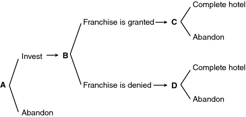
Exhibit 15.1 A Decision Tree for the Sports Hotel
The decision tree models two types of events: the arrival of new information and decisions. Alternative outcomes of decisions are illustrated vertically. Each potential decision is modeled as two or more branches that emanate from a decision node. The starting node in Exhibit 15.1 is labeled A and represents a decision node. A decision node is a point in a decision tree at which the holder of the option must make a decision. In the case of node A, the decision is that the investor must decide whether to start the project. Node B represents an information node. An information node denotes a point in a decision tree at which new information arrives. In the case of node B, the information is the decision by the league as to whether a sports franchise will be granted.
15.1.4 Backward Induction and Decision Trees
Backward induction is used to solve a problem involving options and using a decision tree. Backward induction is the process of solving a decision tree by working from the final nodes toward the first node, based on valuation analysis at each node. Backward induction guides the decision maker to resolve the final decisions first, since those decisions involve a single period and have no real options remaining unresolved. Then, working backward through time one period at a time, the decision maker can resolve decisions until the only remaining decision is the first one. Backward induction is also used in pricing financial derivatives.
Exhibit 15.2 illustrates backward induction. In Exhibit 15.2a, the ends of each path have been valued using the assumed information and based on all possible paths of outcomes and decisions; all uncertainty has been resolved. The analysis now moves to nodes C and D, which are decision nodes representing points in time at which the investor can decide which path to take. The decisions of the investor at nodes C and D can be solved under the continuing and simplifying assumption that the appropriate discount rate is 0%. For example, at node C, the investor would prefer to complete the hotel (receive $30 million), and at node D, the investor would prefer to abandon the hotel (lose only $10 million). These decisions are reflected in Exhibit 15.2b. The process is repeated to value the project at node B, yielding a value of $10 million (multiplying $30 million by 0.5 and multiplying –$10 million by 0.5, and summing). The results are reflected in Exhibit 15.2c.
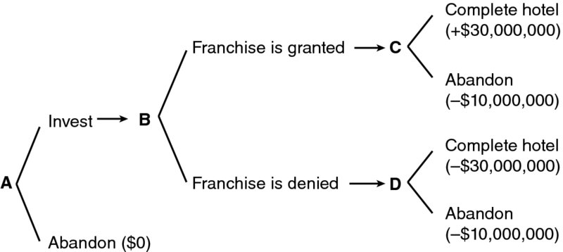
Exhibit 15.2A The Sports Hotel Decision Tree with Final Nodes Valued

Exhibit 15.2B The Sports Hotel Decision Tree with Final Decision Included

Exhibit 15.2C The Sports Hotel Decision Tree with Final Decision and New Information Included
Exhibit 15.2 illustrates that the investor's decision is simple. Proceeding with the first-year plans for the hotel produces an expected profit of $10 million. The project appeared to have no value, meaning expected benefits equaled expected costs, when options were ignored. However, when options are priced, the project has tremendous value. The essential driver of value emanating from an option analysis is the ability to revise plans when new information arrives. Real estate investment involves risk, and real estate development typically involves great risk. However, the risk that a developer might not be able to sell or lease when a real estate development is completed (e.g., because of adverse general market conditions) can be mitigated by preselling or preleasing all or part of the real estate development before its completion. Analysis using real options can help structure the problem such that the value of being able to defer decisions until after new information has arrived and uncertainty has been resolved can be assessed and appreciated.
15.2 Valuation and Risks of Real Estate Equity
Valuation is central to finance and critical to real estate analysis. Real estate valuation is the process of estimating the market value of a property and should be reflective of the price at which informed investors would be willing to both buy and sell that property. In the case of private commercial real estate equity, the assets and their valuations have idiosyncrasies. Valuation challenges arise because the respective assets are not exchange traded, like stocks or bonds of public companies, and also because each real estate asset is unique, with its own risk and return characteristics. Real estate assets are also notorious for their illiquidity, as an individual property may not be traded for a considerable number of years. Nevertheless, in spite of the difficulties, and perhaps because of those difficulties, commercial real estate valuation is necessary.
This section summarizes two approaches used for valuing private commercial real estate equity: the income approach and the comparable sale prices approach. The income approach values real estate by projecting expected income or cash flows, discounting for time and risk, and summing them to form the total value. The comparable sale prices approach values real estate based on transaction values of similar real estate, with adjustments made for differences in characteristics.
Other approaches, such as the profit approach, exist. The profit approach to real estate valuation is typically used for properties with a value driven by the actual business use of the premises; it is effectively a valuation of the business rather than a valuation of the property itself. The profit approach can be used when the value of the property is based primarily on the value of the business that occupies the space.
15.2.1 Cash Flows for the Income Approach
The value of a commercial property depends on the benefits it can offer to its investors. The benefits are the future incomes or, preferably, cash flows that are expected over the life of the property being held as a standing investment. The income approach to real estate valuation consists of forecasting a property's future expected revenues (e.g., rents) and expenses and then discounting the income, which is revenues minus expenses, at an appropriate rate to find an estimate of the property's value. The income approach is also known as the discounted cash flow (DCF) method when cash flows are discounted rather than accounting estimates of income.
Since most properties are unlimited in longevity, cash flows are often projected to some horizon point in time, at which a liquidation value is forecasted. Alternatively, a property may be valued using a perpetuity formula. For long-term horizons, annual values and annual discounting are common.
The investment value (IV) or intrinsic value of the property is based on the discounted expected cash flows, E[CFt], for each time period, t, as illustrated in Equation 15.1:

The final term in the equation is the present value of the net sale proceeds. The net sale proceeds (NSP) is the expected selling price minus any expected selling expenses arising from the sale of the property at time T. In the case of real estate, interim or operating cash flows are usually estimated using the concept of net operating income. Net operating income (NOI) is a measure of periodic earnings that is calculated as the property's rental income minus all expenses associated with maintaining and operating the property. Equating the expected cash flow at time t, E[CFt], with the net operating income, E[NOIt], generates the following equation:

We illustrate the income approach with the following example. Suppose that an investor is considering the purchase of an office building. The potential gross income is the gross income that could potentially be received if all offices in the building were occupied. For this example, the potential gross income of the first year of operations has been estimated at $300,000. However, it is unlikely that the building will be fully occupied all year round. In the case of commercial properties, there typically needs to be some consideration for possible vacancies and therefore the loss of rental income. The vacancy loss rate is the observed or anticipated rate at which potential gross income is reduced for space that is not generating rental income. The effective gross income is the potential gross income reduced for the vacancy loss rate. Assuming a 10% vacancy loss rate and no other income, the effective gross income from the building in the first year will be $300,000 – ($300,000 × 0.1) = $270,000.
To be able to estimate the NOI, the operating expenses arising from the property need to be estimated and then subtracted from the gross income. Operating expenses are non-capital outlays that support rental of the property and can be classified as fixed or variable. Fixed expenses, examples of which are property taxes and property insurance, do not change directly with the level of occupancy of the property. Variable expenses, examples of which are maintenance, repairs, utilities, garbage removal, and supplies, change as the level of occupancy of the property varies. This simplified example does not consider depreciation, which is discussed later. Continuing with the example, assume that fixed and variable expenses were estimated at $42,000 and $75,000, respectively, for a total operating expense of $117,000 for the first year, or 43.3% of the first-year effective gross income. Therefore, the NOI arising from this property in the first year is estimated to be:
or
Now, assuming that the investor expects to maintain the property for seven years, that rents are estimated to increase by 4% per year, that the vacancy loss rate will remain constant at 10%, and that annual operating expenses will continue to represent the same fraction of effective gross income (117/270), the projected annual NOI for each year in the seven-year period is as shown in Exhibit 15.3.
Exhibit 15.3 Estimates of Annual Net Operating Income
Year 1 |
Year 2 |
Year 3 |
Year 4 |
Year 5 |
Year 6 |
Year 7 |
|
| Potential gross income | $300,000 |
$312,000 |
$324,480 |
$337,459 |
$350,958 |
$364,996 |
$379,596 |
| Vacancy loss | −$30,000 |
−$31,200 |
−$32,448 |
−$33,746 |
−$35,096 |
−$36,500 |
−$37,960 |
| Effective gross income | $270,000 |
$280,800 |
$292,032 |
$303,713 |
$315,862 |
$328,496 |
$341,636 |
| Operating expenses | −$117,000 |
−$121,680 |
−$126,547 |
−$131,609 |
−$136,873 |
−$142,348 |
−$148,042 |
| Net operating income | $153,000 |
$159,120 |
$165,485 |
$172,104 |
$178,988 |
$186,148 |
$193,594 |
Finally, assume that the net sale proceeds in year 7 have been estimated at $1,840,000.
15.2.2 Discount Rate for the Income Approach
To be able to calculate the investment value of the office building in the previous section, a discount rate needs to be estimated to compute the present value of the expected cash flows. There are several approaches that can be used to estimate an appropriate discount rate. In the case of real estate investments, the discount rate is often estimated using a risk premium approach. The risk premium approach to estimation of a discount rate for an investment uses the sum of a riskless interest rate and one or more expected rewards—expressed as rates—for bearing the risks of the investment. The following formulas use a risk premium approach with two risk premiums: one for liquidity and one for risk.
where r is the required return on the respective real estate investment, Rf is the risk-free rate of return (the return or yield on a Treasury security of similar maturity to the real estate investment), E(RLP) is a liquidity premium that is inherent to direct real estate investments, and E(RRP) is the required risk premium or extra return demanded for bearing the remaining risks of investing in the specific real estate project.
Equation 15.3 expresses r using a multiplicative relationship that generates a generally more accurate measure of r using traditional interest rate conventions and annual compounding. Equation 15.4 expresses r as an approximation. The three summed components on the right-hand side of Equation 15.4 ignore the cross products of Rf and the risk premiums. For many situations, the approximation is adequate.
Using a discount rate of 9%, the investment value of the office building is as follows:

In practice, the cash flow estimates typically involve a far more detailed projection of cash flows than were illustrated in the example. Full pro forma appraisals usually incorporate the following key elements: rental income on a lease-by-lease basis, other sources of income, a deduction for factors such as allowances for unanticipated vacancies and downtime between leases in a given space, detailed operating expenses, capital items, tenant improvements, and leasing commissions.
For large properties, rental income calculations can become complicated if the property has multiple leases. In such a case, total rental income is estimated by calculating and summing the annual rental income received for each lease in the property. Future demand-and-supply dynamics in the relevant real estate market and the impact of market conditions on the cash flows of the property are vital concerns. As the largest factor in the cash flows will be the net rental income, rent estimates must be as unbiased as possible. A simplistic approach is to assume that rents will increase through all of the years at an estimated and fixed rate of growth that reflects anticipated inflation and any other relevant factors.
The operating expenses incurred by the property include a wide variety of items. Some of them, such as general property management expenses, are recurring and contracted and can therefore be regarded as fixed expenses. Other expenses are considered variable because they depend on the level of property vacancy. It is important to take into consideration the terms of the leases, as some leases may be gross and some may be net. In a net lease, the tenant is responsible for almost all of the operating expenses.
The other major expense items on the pro forma cash flow are primarily related to capital improvements and leasing costs. These are irregular payments that are dependent on such factors as the terms of the lease and the condition of the property. In addition, it is common to include a capital reserve for the anticipated level of unexpected costs.
The issue of tenant improvements depends on the exact nature of the property. However, office and retail space is generally offered in such a condition as to allow tenants to tailor it to their own needs. It is common for a landlord to at least partially contribute to these fitting-out costs. The extent to which this is a major cost largely depends not only on the magnitude of the costs but also on the frequency of tenant turnover in the property. The final major item is leasing commissions, which are the costs payable to the brokerage firm for marketing the space.
There are other important issues in applying the DCF approach. First, there is a difference between income and cash flow, especially with real estate when depreciation is involved. Depreciation is a noncash expense that is deducted from revenues in computing accounting income to indicate the decline of an asset's value. To convert income to cash flow, it is necessary to add depreciation back into income. Importantly, depreciation is tax deductible, and its role in decreasing taxable income and increasing after-tax cash flows is essential to the analysis. The importance of depreciation for taxable investors is detailed later in this chapter.
15.2.3 Taxes and Financing Costs in the Income Approach
The example in Exhibit 15.3 ignored income taxes and implicitly used a required rate of return that would be appropriate for pre-tax cash flows. In the case of institutional investors without income taxes, there is no need to incorporate taxes. For investors subject to income taxes, there are two ways to view income taxation.
The pre-tax discounting approach is commonly used in finance, where pre-tax cash flows are used in the numerator of the present value analysis (as the cash flows to be received), and the pre-tax discount rate is used in the denominator. An alternative is to use an after-tax approach. In an after-tax discounting approach, the estimated after-tax cash flows (e.g., after-tax bond payments) are discounted using a rate that has been reduced to reflect the net rate received by an investor with a specified marginal tax rate.
Note that in this simplified example, the investor's required after-tax rate of return was simply the pre-tax required rate of return reduced for the tax rate being applied to the cash flows. Further, every cash flow except the final return of the investment was taxed at the same rate, which caused the two approaches to generate identical results. In more realistic scenarios, the taxability of different cash flows and the tax rate of the investor are likely to vary through time.
The pre-tax analysis in the simplified example contains a theoretically inconsistent feature. The $80 coupon payments and $1,000 principal payment to a taxable investor are all discounted at the same high rate (8%) in order to adjust for the effect of taxes. In theory, it is inappropriate to adjust for taxes by attaching a higher discount rate to both the coupon payments and the principal payment because only the coupon payments are taxed. Care should be exercised in interpreting the pre-tax yield in the case of a taxable investor. Nevertheless, both approaches are used in fixed-income analysis.
Finally, the example using Exhibit 15.3 ignored financing flows, such as interest payments and principal payments on a mortgage. The approach valued ownership of the entire real estate property as if there were no mortgage on the property. If there is a mortgage on the property, then the resulting value ($1,863,772) should be equal to the sum of the values of the property's mortgage and equity. The value of the equity in the property could then be estimated as $1,863,772 minus the value of the mortgage. An alternative approach, often termed the equity residual approach, focuses on the perspective of the equity investor by subtracting the interest expense and other cash outflows due to mortgage holders (in the numerator) and by discounting the remaining cash flows using an interest rate reflective of the required rate of return on the equity of a leveraged real estate investment (in the denominator). The resulting value would estimate the value of the equity in the real estate project.
In summary, the income or DCF approach involves projecting all cash flows, including a terminal value (net sale proceeds), and discounting the cash flows using a rate commensurate with the investment's longevity and risk. The accuracy of the approach depends on the accuracy of the cash flow projections and the accuracy of the estimation of the discount rate (required rate of return).
15.2.4 Valuations Based on Comparable Sale Prices
For non-income-producing properties, such as an owner-occupied single-family residence, a DCF approach is not viable. In these cases for which sufficient transaction data are available, valuations are typically based on the comparable sale prices approach. The comparable sale prices approach involves collecting data on the prices at which real estate has traded for properties that are closely related to the property being appraised and that were traded as recently as possible. Since each observed sale will differ from the property being analyzed in terms of property characteristics and/or the time of sale, the professional needs to use judgment and market-based evidence to make appropriate adjustments to the observed prices when estimating an appraised value.
For some properties, a reasonable number of recent sales may be available from reasonably comparable properties. For example, transactions of midsize single-family houses in a relatively large and homogeneous area may provide a reasonable basis for applying the comparable sale prices approach to the valuation of a midsize single-family house in the same area.
However, the comparable sale prices approach is not viable when the number of recent and relevant real estate transactions is very limited. This can occur for highly specialized properties, such as industrial properties that are highly specific in their use, or properties of large scale that cannot be compared in terms of zoning, topography, and other factors that influence value. An alternative approach in these cases is based on two components: (1) the replacement construction costs of the structure, and (2) indications of the market value of the site, assuming it is being employed for its most profitable use.
15.3 Alternative Real Estate Investment Vehicles
Several alternative real estate investment vehicles are available, some of which have been recently introduced. (New alternative real estate investment vehicles are anticipated to be launched in the coming years.) These alternative investments include both private and exchange-traded products. This section begins by discussing the main characteristics of the following private real estate alternative investments: commingled real estate funds, syndications, joint ventures, and limited partnerships. The remainder of the section focuses on public real estate investments, including open-end real estate mutual funds, closed-end real estate mutual funds, and equity real estate investment trusts (REITs).
15.3.1 Private Equity Real Estate Funds
Private equity real estate funds are privately organized funds that are similar to other alternative investment funds, such as private equity funds and hedge funds, yet have real estate as their underlying asset. Three specific types of private equity real estate funds (commingled real estate funds, syndications, and joint ventures) are discussed in the sections that follow. These funds collect capital from investors with the objective of investing in the equity or the debt side of the private real estate space. The funds follow active management real estate investment strategies, often including property development or redevelopment. Private equity real estate funds usually have a life span of 10 years: a two- to three-year investment period and a subsequent holding period during which the properties are expected to be sold.
The primary advantage to an investor is the access to private real estate, especially useful for smaller institutions that are limited in the size of the real estate portfolios they are able to construct directly. However, even for larger institutions, there are advantages to investments in private equity real estate funds (and also to commingled real estate funds, explained in the next section), as these investment vehicles can provide access to larger properties in which an institution may be reluctant to invest alone because of the unique asset risk it would need to bear and because a single asset could account for a portfolio allocation that might be too high. The use of private equity real estate funds can also provide access to local or specialized management or to specific sectors and markets in which the institution does not feel it has sufficient market knowledge or expertise.
However, investments through private equity funds do not allow investors direct control over the real estate portfolio and its management. In addition to the loss of control, private equity fund investors often lack a sufficiently liquid exit route. Another major issue with private equity funds is the difficulty of reporting the values of the underlying properties. Hence, the reported performance may not be accurate, and there may be considerable time or uncertainty in realizing reported performance. The finite life of this vehicle tends to make the funds a “hold to liquidation” instrument.
15.3.2 Commingled Real Estate Funds
Commingled real estate funds (CREFs) are a type of private equity real estate fund that is a pool of investment capital raised from private placements that are commingled to purchase commercial properties. The investors are primarily large financial institutions that receive a negotiable, although non-exchange-traded, ownership certificate that represents a proportionate share of the real estate assets owned by the fund. Generally, CREFs are closed-end in structure (i.e., without additional shares issued or old shares redeemed), with unit values reported through annual or quarterly appraisals of the underlying properties. Other than the negotiability of the ownership certificates, the advantages and disadvantages of CREFs are similar to those of other private equity real estate funds.
15.3.3 Syndications
Syndications are private equity real estate funds formed by a group of investors who retain a real estate expert with the intention of undertaking a particular real estate project. A syndicate can be created to develop, acquire, operate, manage, or market real estate investments. Legally, real estate syndications may operate as REITs, as corporations, or as limited or general partnerships. Most real estate syndications are structured as limited partnerships, with the syndicator performing as general partner and the investors performing as limited partners. This structure facilitates the passing through of depreciation deductions, which are normally high, directly to individual investors, and potentially circumvents double taxation.
Syndications are usually initiated by developers who require extra equity capital to raise money to begin a project. Syndications can be a form of financing that offers smaller investors the opportunity to invest in real estate projects that would otherwise be outside their financial and management competencies. Syndicators profit from both the fees they collect for their services and the interest they may preserve in the syndicated property.
15.3.4 Joint Ventures
Real estate joint ventures are private equity real estate funds that consist of the combination of two or more parties, typically represented by a small number of individual or institutional investors, embarking on a business enterprise such as the development of real estate properties. An example of a joint venture would be the case of an institutional investor with an interest in investing in real estate, but with no expertise in this area, that agrees to form a joint venture with a developer. A joint venture can be structured as a limited partnership, an important form of real estate investment that is explained in the next section.
15.3.5 Limited Partnerships
Private equity real estate funds, including the three types described in the previous sections, are increasingly organized as limited partnerships. Not only have real estate funds increasingly adopted limited partnership structures, but existing limited partnerships—such as private equity and hedge funds—have increasingly entered the real estate market. As with other limited partnership structures, a private real estate equity fund's sponsors act as the general partner and raise capital from institutional investors, such as pension funds, endowments, and high-net-worth individuals, who serve as limited partners. Generally, the initial capital raised is in the form of commitments that are drawn down only when suitable investments have been identified.
Limited partnership funds in real estate have largely adopted a more aggressive investment, reflected by gearing. Gearing is the use of leverage. The degree of gearing can be expressed using a variety of ratios. In real estate funds, a popular gearing ratio is the percentage of a fund's capital that is financed by debt divided by the percentage of all long-term financing (e.g., debt plus equity). This ratio is often called the LTV (loan-to-value) ratio or the debt-to-assets ratio. Many traditional real estate funds have limited, if any, gearing, whereas a large proportion of the new private equity real estate limited partnerships have LTVs as high as 75%. Gearing ratios are also commonly expressed as the ratio of debt to equity.
Limited partnerships have also tended to adopt the fee structures commonly in place in private equity funds. In addition to an annual management fee, commonly in the region of 1% to 2% of assets under management, the newer funds have introduced performance-related fees, commonly in the region of 20% of returns. Generally, the incentive-based performance fees are subject to some form of hurdle rate or preferred return. The fund sponsors (or general partners) usually contribute some capital to the fund (e.g., 8% to 10%), thus potentially benefiting not only from the explicit incentive and management fees but also from their share of the limited partnership's return through their investments.
15.3.6 Open-End Real Estate Mutual Funds
Open-end real estate mutual funds are public investments that offer a non-exchange-traded means of obtaining access to the private real estate market. These funds are operated by an investment company that collects money from shareholders and invests in real estate assets following a set of objectives laid out in the fund's prospectus. Open-end funds initially raise money by selling shares of the funds to the public and generally continue to sell shares to the public when requested. Open-end real estate mutual funds allow investors to gain access to real estate investments with relatively small quantities of capital. These funds often allow investors to exit the fund freely by redeeming their shares (potentially subject to fees and limitations) at the fund's net asset value, which is computed on a daily basis.
However, these funds may limit investors' ability to redeem units and exit the fund when, for example, a significant percentage of shareholders wish to redeem their investments and the fund is encountering liquidity problems. These liquidity problems can be exacerbated when the real estate market is either booming or declining. Given that upward and downward phases in real estate prices may last a considerable length of time, some analysts may view real estate valuations used in some net asset value computations as trailing true market prices in a bull market (and trailing declines in a bear market).
The use of prices that lag changes in true market prices is known as stale pricing. Stale pricing of the net asset value of a fund provides an incentive for existing shareholders to exit (sell) during declining markets and new investors to enter (buy) during rising markets. These actions of investors exploiting stale pricing may be viewed as transferring wealth from long-term shareholders in the fund to the investors exploiting the stale prices. The reason that the purchase transactions in a rising market transfer wealth from existing shareholders to new shareholders is that the stale prices are artificially low and permit new shareholders to receive part of the profit when the fund's net asset value catches up to its true value. Conversely, sales transactions during declining markets transfer wealth from remaining shareholders to exiting shareholders because the stale prices are artificially high and permit the exiting shareholders to receive proceeds that do not fully recognize the true losses, leaving the true losses to be disproportionately borne by the remaining shareholders when the fund's net asset value falls to its true value.
During declining markets, an open-end fund may face redemption problems and be forced to sell some of its real estate assets at deep discounts to obtain liquidity. To protect long-term investors and fund assets, many open-end real estate mutual funds increasingly opt to reserve the right to defer redemption by investors to allow sufficient time to liquidate assets in case they need to do so.
In summary, investors in open-end mutual funds are typically offered daily opportunities to redeem their outstanding shares directly from the fund or to purchase additional and newly issued shares in the fund. This attempt to have high liquidity of open-end real estate fund shares contrasts with the illiquidity of the underlying real estate assets held in the fund's portfolio. This liquidity mismatch raises issues about the extent to which investors will receive liquidity when they need it most and whether realized returns of some investors will be affected by the exit and entrance of other investors who are timing or arbitraging stale prices.
15.3.7 Options and Futures on Real Estate Indices
Derivative products allow investors to transfer risk exposure related to either the equity side or the debt side of real estate investments without having to actually buy or sell the underlying properties. This is accomplished by linking the payoff of the derivative to the performance of a real estate return index, thus allowing investors to obtain exposures without engaging in real estate property transactions or real estate financing.
Challenges to real estate derivative pricing and trading include difficulties that arise with the highly heterogeneous and illiquid assets comprising the indices that underlie the derivative contracts. The indices underlying the derivatives may not correlate highly to the risk exposures faced by market participants, and therefore use of the derivatives for hedging may introduce basis risk, discussed in Chapter 12. Nevertheless, real estate derivatives may offer the potential for increased transparency and liquidity in the real estate market.
15.3.8 Exchange-Traded Funds Based on Real Estate Indices
Exchange-traded funds (ETFs) represent a tradable investment vehicle that tracks a particular index or portfolio by holding its constituent assets or a subsample of them. They trade on exchanges at approximately the same price as the net asset value of the underlying assets due to provisions that allow for the creation and redemption of shares at the ETF's net asset value. The actions of speculators attempting to earn arbitrage profits by creating and selling ETF shares when they appear overpriced in the market or buying and redeeming ETF shares when they appear underpriced in the market tend to keep ETF market prices within a narrow band of the underlying value of the ETF. These funds have the advantage of being a relatively low-trading-cost investment vehicle (in the case of those ETFs that have reached a particular size or popularity among investors); they can be tax efficient; and they offer stock-like features, such as liquidity, dividends, the possibility to go short or to use with margin, and, in some cases, the availability of calls and puts. Exchange-traded funds based on real estate indices track a real estate index such as the Dow Jones U.S. Real Estate Index, which raises issues of basis risk to hedgers. Other ETFs, such as the FTSE NAREIT Residential, track a REITs index. Since REITs are publicly traded, the use of ETFs on REITs may offer cost-effective diversification but may not offer substantially distinct hedging or speculation opportunities.
15.3.9 Closed-End Real Estate Mutual Funds
A closed-end fund is an exchange-traded mutual fund that has a fixed number of shares outstanding. Closed-end funds issue a fixed number of shares to the general public in an initial public offering, and in contrast to the case of open-end mutual funds, shares in closed-end funds cannot be obtained from or redeemed by the investment company. Instead, shares in closed-end funds are traded on stock exchanges.
A closed-end real estate mutual fund is an investment pool that has real estate as its underlying asset and a relatively fixed number of outstanding shares. Unlike open-end funds, closed-end funds do not need to maintain liquidity to redeem shares, and they do not need to establish a net asset value at which entering and exiting investors can transact with the investment company. Most important, unlike with open-end funds, the closed-end funds themselves and their existing shareholders are not disrupted by shareholders entering and exiting the fund, especially in an attempt to arbitrage stale prices. This is because shareholders buy and sell shares on secondary markets rather than affecting fund liquidity by redeeming shares or subscribing to new shares.
Since closed-end funds are not required to meet shareholder redemption requests, the fund structure is generally more suitable for the use of leverage than that of open-end funds. The closed-end structure is frequently used to hold assets that investors often prefer to hold with leverage, such as municipal bonds. Similarly, the closed-end fund structure has advantages for investment in relatively illiquid assets, and is often used for such assets as real estate and emerging market stocks.
Like other closed-end funds, closed-end real estate mutual funds often trade at premiums or substantial discounts to their net asset values, especially when net asset values are not based on REITs, since REITs have market values. Closed-end real estate mutual funds usually liquidate their real estate portfolios and return capital to shareholders after an investment term (typically 15 years), the length of which is stated at the fund's inception.
15.3.10 Equity Real Estate Investment Trusts
This introduction to public equity real estate investment products concludes with a discussion of equity REITs. As introduced and briefly described in Chapter 14, REITs are a popular form of financial intermediation in the United States. This discussion focuses on equity REITs, which are REITs with a majority of their underlying real estate holdings representing equity claims on real estate rather than mortgage claims.
An equity REIT acquires, renovates, develops, and manages real estate properties. It produces revenue for its investors primarily from the rental and lease payments it receives as the landlord of the properties it owns. An equity REIT also benefits from the appreciation in value of the properties it owns as well as any increase in rents. In fact, one of the benefits of equity REITs is that their rental and lease receipts tend to increase along with inflation, making REITs a potential hedge against inflation.
One of the biggest advantages is that REITs are publicly traded. Most REITs fall into the capitalization range of $500 million to $5 billion, a range typically associated with small-cap stocks and the smaller half of mid-cap stocks. The market returns on equity REITs have been observed to have a strong correlation with equity market returns, especially the returns of small-cap stocks (and to a slightly lesser extent those of mid-cap stocks).
The strong correlation of equity REIT returns with the returns of similarly sized operating firms raises a very important issue. Are the returns of equity REITs highly correlated with the returns of small stocks because the underlying real estate assets are highly correlated with the underlying assets of small stocks? Or is this correlation due to the similar sizes (total capitalization values) of REITs and small-cap stocks and the fact that they are listed on the same exchanges? The explanation that REIT returns are highly correlated with the returns of similarly sized operating firms due to the similarity of the risks of their underlying assets seems dubious.
Commercial real estate valuations tend to depend on projected rental income, whereas operating firm valuations tend to depend on sales of products and services that are generally unrelated to real estate. However, the idea that the shared size and shared financial markets explain the correlation runs counter to traditional efficient capital market theory. Financial theory implies that market prices reflect underlying economic fundamentals rather than trading location and size or total capitalization. To the extent that REIT prices are substantially influenced by the nature of their trading would mean that observed returns are more indicative of stock market fluctuations and less indicative of changes in underlying real estate valuations. However, due to problems with other approaches (as addressed in a subsequent section), REIT returns form the basis for the empirical analyses presented at the end of this chapter.
15.4 Real Estate and Depreciation
The tax implications of depreciation expense are important in real estate investing. Especially when leveraged, the effects of income taxes on real estate returns can be substantial, and can often cause real estate to be prized as a highly tax-advantaged investment opportunity. Taxable investors have obvious reasons to analyze the tax advantages, but even non-taxable investors should be aware of the tax implications of depreciation, because the market prices of investments with large tax advantages will tend to be relatively high. Tax-free investors should be concerned about implicitly paying for these benefits when they are embedded in real estate prices.
Outlays of cash by real estate investors include capital expenditures on capital assets, expenses, and capital flows, such as principal payments on debt. In the United States and in many other jurisdictions, expenses are tax-deductible in the current year and therefore generate a prompt reduction in cash outflows through reduced income taxes. Capital expenditures are generally not immediately tax-deductible and therefore do not generally produce the benefit of an immediate reduction in taxable income and taxes. Rather, purchasers of capital assets do not receive tax deductions on the expenditure until and unless the asset is depreciated.
For taxable investors, when depreciation expense can be deducted from revenues in determining income taxes, the depreciation expense can substantially increase after-tax cash flows and after-tax rates of return. Buildings are generally depreciable, but land is not. Depreciation was not included in the simplified example depicted in Exhibit 15.3. However, for a taxable investor, depreciation is an important item in the determination of taxable income, in the relationship between income and cash flow, and in the determination of income taxes. This section takes a closer look at the effect of depreciation methods on after-tax returns by analyzing a stylized example. This section illustrates four important principles regarding the effects of depreciation rates on the relationship between pre-tax and after-tax rates of return. The purpose is to show the effect of the rate at which an asset is allowed to be depreciated on the after-tax internal rate of return (IRR) generated by the asset.
15.4.1 Real Estate Example without Taxation
Consider a real estate property that cost $100 million and will be sold after three years. For simplicity, ignore inflation and assume that the true value of the property will decline by 10% each year due to wear and aging. Assume that the cash flows generated by the property each year are equal to the sum of 10% of the property's value at the end of the previous year plus the amount by which the property declined in value. For example, operating cash flow at the end of year 1 is equal to $20 million, found as 10% of $100 million plus the difference between $100 million and $90 million. These numbers are illustrated in Exhibit 15.4 and are constructed to generate a 10% IRR on a pre-tax basis. The 10% IRR should be expected because the assets earn 10% above and beyond depreciation each year. The IRR is computed using the initial investment ($100 million), the operating cash flows for each year, and the assumption that the property can be sold at the end of the third year at its year 3 value ($72.90 million).
Exhibit 15.4 A Stylized Depreciable Real Estate Property: No Taxes ($ in millions)
| End of Year 0 | End of Year 1 | End of Year 2 | End of Year 3 | |
| True property value | $100.00 | $90.00 | $81.00 | $72.90 |
| Operating cash flow | $0 | $20.00 | $18.00 | $16.20 |
| − Depreciation | $0 | −$10.00 | −$9.00 | −$8.10 |
| − Taxes | $0 | $0 | $0 | $0 |
| Net income | $0 | $10.00 | $9.00 | $8.10 |
| Sales proceeds | $72.90 | |||
| Total cash flow | −$100.00 | $20.00 | $18.00 | $89.10 |
| IRR = 10.0% |
15.4.2 After-Tax Returns When Depreciation Is Not Allowed
This section continues with the previous real estate example and modifies the example to include taxation at a stated rate of 40% of income. A stated rate of income tax is the statutory income tax rate applied to reported income each period. The stated tax rate can differ from the effective tax rate. The effective tax rate is the actual reduction in value that occurs in practice when other aspects of taxation are included in the analysis, such as exemptions, penalties, and timing of cash flows. For example, a corporation with $100 million of taxable income that is taxed at a 10% statutory rate would experience a lower effective tax rate if the tax law granted the corporation the opportunity to pay the taxes several years later and without penalty.
To include taxation without depreciation, assume that the operating cash flows from each year are fully taxed, even though the cash flows overstate the income because the value of the property is declining through time. In other words, depreciation expense is not allowed for tax purposes in this example. Depreciation may be viewed as a way of marking an asset to market. If the property were marked-to-market in the first year, the $20 million of operating cash flow would not be fully taxed, since the process of marking the property's value to market would generate a $10 million offsetting loss through depreciation.
Exhibit 15.5 illustrates the incomes and cash flows. The property is sold at a loss to its initial purchase price. Because depreciation is not allowed, assume that this loss is allowed to offset the investor's taxable income in that year, thereby generating reduced taxes in the third year. Assume through this section that the investor has sufficient income from other investments to utilize any tax losses generated by this investment.
Exhibit 15.5 A Stylized Depreciable Real Estate Property: No Depreciation ($ in millions)
| End of Year 0 | End of Year 1 | End of Year 2 | End of Year 3 | |
| True property value | −$100.00 | −$90.00 | −$81.00 | −$72.90 |
| Operating cash flow | $0 | −$20.00 | −$18.00 | −$16.20 |
| Pre-tax profit | $0 | −$20.00 | −$18.00 | −$16.20 |
| − Taxes | $0 | −$8.00 | −$7.20 | −$6.48 |
| Net income | $0 | −$12.00 | −$10.80 | −$9.72 |
| Sales proceeds | −$72.90 | |||
| Capital loss tax shield (40% of loss) | −$10.84 | |||
| Total cash flow | −$100.00 | −$12.00 | −$10.80 | −$93.46 |
| IRR = 5.8% |
Depreciation, which is not included in Exhibit 15.5, can have a substantial effect on measured performance. Depreciation as a measure of the decline in the value of an asset can be either an estimation of the true economic decline that the asset experiences or an accounting value based on accounting conventions.
As indicated in Exhibit 15.5, the after-tax IRR of the property is 5.8%. Note that the after-tax IRR is less than 6%, which would be 60% of the 10% pre-tax IRR. This result illustrates the first principle of depreciation and returns: When accounting depreciation either is not allowed for tax purposes or is allowed at a rate that is slower than the true economic depreciation, the after-tax IRR will be less than the pre-tax IRR reduced by the tax rate. In this example, the pre-tax IRR of 10% reduced by the tax rate of 40% is 6%. The actual after-tax IRR of 5.8% is more than 40% lower than the pre-tax IRR, demonstrating that the present value of the taxes exceeds 40% of the present value of the profits. Thus when depreciation for tax accounting purposes either is not allowed or is allowed on a deferred basis relative to true economic depreciation, the after-tax return will generally be less than the pre-tax return reduced by the stated income tax rate.
The intuition of the first principle is that by disallowing a deduction for depreciation on a timely basis, the investor is, in an economic sense, paying taxes before they are due. The investor may be viewed as providing an interest-free loan to the government by paying taxes in advance of when the taxes would be paid if the investor were being taxed on true economic income as it occurred. Thus, the effective tax rate exceeds the stated tax rate.
15.4.3 Return When Accounting Depreciation Equals Economic Depreciation
This section continues with the real estate example of the previous two sections and modifies the example to include depreciation for tax accounting purposes that is allowed at a rate that matches the true economic depreciation of decline in the value of the property. Exhibit 15.6 illustrates the incomes and cash flows. Since the property is sold at its depreciated value, there is no income tax due on its sale.
Exhibit 15.6 A Stylized Depreciable Real Estate Property: Economic Depreciation ($ in millions)
| End of Year 0 | End of Year 1 | End of Year 2 | End of Year 3 | |
| True property value | −$100.00 | $90.00 | $81.00 | $72.90 |
| Operating cash flow | $0 | $20.00 | $18.00 | $16.20 |
| − Depreciation | $0 | −$10.00 | −$9.00 | −$8.10 |
| Pre-tax profit | $0 | $10.00 | $9.00 | $8.10 |
| − Taxes | $0 | −$4.00 | −$3.60 | −$3.24 |
| Net income | $0 | $6.00 | $5.40 | $4.86 |
| Sales proceeds | $72.90 | |||
| Total cash flow | −$100.00 | $16.00 | $14.40 | $85.86 |
| IRR = 6.0% |
As indicated in Exhibit 15.6, the after-tax IRR of the property is 6%. Note that this after-tax IRR is exactly 60% of the pre-tax IRR (10%). In other words, a stated income tax rate of 40% causes a 40% reduction in the IRR earned by the investor, so the effective tax rate equals the stated tax rate. This illustrates the second principle of depreciation and returns: When depreciation for tax accounting purposes matches true economic depreciation in timing, the after-tax return generally equals the pre-tax return reduced by the stated income tax rate.
It should be noted that the speed of the depreciation method does not affect the aggregated taxable income (summed through all of the years). Rather, the rate of the depreciation changes the timing of the taxes. When the time value of money is included, the rate of the depreciation changes the after-tax IRR and the effective tax rate.
15.4.4 Return When Accounting Depreciation Is Accelerated
This section demonstrates the most common situation in practice: Accounting depreciation for tax purposes is allowed to write off the value of an asset more quickly than it is actually declining in value. In fact, in practice, it is typically the case that accounting depreciation for tax purposes writes off the value of real estate assets that are actually increasing in value through time. For simplicity, accelerated depreciation is modeled as $20 million in each of the first three years. Exhibit 15.7 illustrates the incomes and cash flows. Since the property is sold above its depreciated value, there is income tax due on its sale.
Exhibit 15.7 A Stylized Depreciable Real Estate Property: Accelerated Depreciation ($ in millions)
| End of Year 0 | End of Year 1 | End of Year 2 | End of Year 3 | |
| True property value | $100.00 | $90.00 | $81.00 | $72.90 |
| Operating cash flow | $0 | $20.00 | $18.00 | $16.20 |
| Profit before depreciation | $0 | $20.00 | $18.00 | $16.20 |
| − Depreciation | $0 | −$20.00 | −$20.00 | −$20.00 |
| Pre-tax profit | $0 | $0 | −$2.00 | −$3.80 |
| − Taxes | $0 | $0 | $0.80 | $1.52 |
| Net income | $0 | $0 | −$1.20 | −$2.28 |
| Book value end of period | $100.00 | $80.00 | $60.00 | $40.00 |
| Sales proceeds | $72.90 | |||
| − Capital gain taxes (40% of profit) | −$13.16 | |||
| Total cash flow | −$100.00 | $20.00 | $18.80 | $77.46 |
| IRR = 6.3% |
As indicated in Exhibit 15.7, the after-tax IRR of the property is 6.3%. Accelerated depreciation, shown in Exhibit 15.5, generates an after-tax IRR that exceeds the after-tax IRR that was found in Exhibit 15.6 when accounting depreciation matched the true economic depreciation. The reason is that accelerated depreciation defers income taxes, effectively serving as an interest-free loan from the government to the investor, enhancing the value of the property. The resulting effective tax rate is less than the stated tax rate. This illustrates the third principle of depreciation and returns: When depreciation for tax accounting purposes is accelerated in time relative to true economic depreciation, the after-tax return generally exceeds the pre-tax return reduced by the stated income tax rate.
15.4.5 Return When Capital Expenditures Can Be Expensed
This section analyzes an extreme situation in which capital expenditures are allowed to be immediately and fully deducted, or expensed, for income tax purposes. Such treatment is generally allowed for smaller and shorter-term assets, such as minor equipment, but not for real estate. The point here is to illustrate the most extreme possible form of accelerated depreciation. Exhibit 15.8 illustrates the incomes and cash flows. The initial purchase price of $100 million can be expensed, generating $40 million of tax savings (i.e., offsets to the investors' other taxable income). Since the property is sold above its depreciated value ($0), there is income tax due on the full proceeds of its sale.
Exhibit 15.8 A Stylized Depreciable Real Estate Property: Expensed ($ in millions)
| End of Year 0 | End of Year 1 | End of Year 2 | End of Year 3 | |
| True property value | $100.00 | $90.00 | $81.00 | $72.90 |
| Operating cash flow | −$100.00 | $20.00 | $18.00 | $16.20 |
| Pre-tax profit | −$100.00 | $20.00 | $18.00 | $16.20 |
| − Taxes | $40.00 | −$8.00 | −$7.20 | −$6.48 |
| Net income | $0 | $12.00 | $10.80 | $9.72 |
| Sales proceeds | $72.90 | |||
| − Capital gain taxes (40% of profit) | −$29.16 | |||
| Total cash flow | −$60.00 | $12.00 | $10.80 | $53.46 |
| IRR = 10% |
As indicated in Exhibit 15.8, the after-tax IRR of the property is 10%. Amazingly, being able to expense outlays immediately on an investment causes the after-tax IRR to equal the pre-tax IRR (10%). The intuition is that all cash inflows and outflows are reduced by 40%. The scale of the cash flows is reduced, but the relative values and timing do not change. Thus, the IRRs of the pre-tax and after-tax cash flows are the same. In practice, major capital expenditures can typically not be expensed in the year of purchase. However, the case parallels the benefits of fully tax-deductible retirement investing. This illustrates the fourth principle of depreciation and returns: When all investment outlays can be fully and instantly expensed for tax accounting purposes, the after-tax return generally equals the pre-tax return.
The reduced taxation afforded by depreciation is due to the depreciation tax shield. A depreciation tax shield is a taxable entity's ability to reduce taxes by deducting depreciation in the computation of taxable income. The present value of the depreciation tax shield is the present value of the tax savings generated by the stream of depreciation. Real estate equity investment tends to offer substantial depreciation tax shields to taxable investors.
The above discussions regarding depreciation and taxes have shown that when depreciation for tax accounting purposes occurs at the same rate as true economic decline in the value of the asset, the value of the depreciation tax shield drives the effective tax rate to equal the stated tax rate. In other words, the after-tax IRR will equal the pre-tax IRR reduced by the stated tax rate. However, as is often the case, when real estate depreciation for tax purposes is allowed to substantially exceed the true economic depreciation, the value of the depreciation tax shield can cause the effective income tax rate on the property to be substantially lower than the stated tax rate.
15.4.6 Summary of Depreciation and Taxes
As an alternative asset, real estate requires specialized analysis. Depreciation is a noncash expense that can have important effects on taxes and after-tax rates of return. Generally, real estate buildings offer taxable investors in the equity of the real estate the opportunity to receive a depreciation tax shield that can be very valuable and needs to be considered in decision-making. Most equity positions in real estate possess average to above-average income tax benefits.
Competition should drive the prices and expected returns of investments to reflect the taxability of the investment's income. Entities in zero or low income tax brackets should generally prefer investments that are highly taxed, whereas investors in high income tax brackets should prefer investments that offer income tax advantages, such as the opportunity to claim accelerated depreciation. Tax-exempt investors and investors in very low income tax brackets may find the rates of return on equity real estate to be insufficient to support equally high asset allocations to real estate. Nevertheless, substantial real estate is held by and typically should be held by tax-exempt investors due to the other advantages offered by real estate.
15.5 Real Estate Equity Risks and Returns
Most real estate is privately owned and privately traded. Thus, observation and measurement of real estate prices are problematic. There are three general approaches to computing indices of real estate returns: (1) appraisals, (2) adjusted privately traded prices, and (3) financial market prices. In practice, some applications are a combination of these three approaches.
15.5.1 Real Estate Indices Based on Appraisals
Privately held real estate values can be appraised (estimated professionally) and used as a basis for a price index. The NCREIF Property Index (NPI) is the primary example of an appraisal-based real estate index in the United States and is published by the National Council of Real Estate Investment Fiduciaries (NCREIF), a not-for-profit industry association that collects data regarding property values from its members. Every quarter, members of NCREIF are required to submit their data about the value of the real estate properties they own to support the computation of the NPI. Then NCREIF aggregates this information from its members on a confidential basis, builds price indices based on these data, and publishes these indices.
The NPI is frequently used as a proxy for the performance of direct investments in commercial real property. More specifically, it proxies the returns for an institutional-grade real estate portfolio held by large U.S. investors. In addition, NCREIF publishes sub-indices. For example, NCREIF offers a breakdown by the types of properties underlying the NPI, including offices, apartments, industrial properties, and retail. Collectively, these types of properties form the core of institutional real estate portfolios.
The NPI is calculated on an unleveraged basis, as if the property being measured were purchased with 100% equity and no debt, so the returns are less volatile than returns to equity investment in real estate that contain leverage, and no interest charges are deducted. The returns to the NPI are calculated on a before-tax basis and therefore do not include income tax effects. Finally, the returns are calculated for each individual property and then are value-weighted in the index calculation.
NCREIF indices are based on appraisals. Appraisals are professional opinions with regard to the value of an asset, such as a real estate property. The appraised values of real estate properties are generally based on analysis using two methods: the comparable sales method or the DCF method. Both methods were detailed in previous sections of this chapter. The DCF method has become the more accepted practice by real estate appraisers for commercial real estate.
The members of NCREIF report the value of their properties every quarter based on these appraisals. Although the NPI is reported quarterly, NPI properties are not necessarily appraised every quarter. Most properties are valued once per year, but some are appraised only every two or three years. The reason is that appraisals cost money, and therefore there is a trade-off between the benefits of having frequent property valuations and the costs of those valuations. Instead of conducting a full revaluation of the property, property owners may simply adjust its value for any additional capital expenditures. In fact, many institutional real estate investors revalue their portfolio properties only when they believe there is a substantial change in value based on new leases, changing economic conditions, or the sale of a similar property close to the portfolio property. Even when appraisals can be performed frequently and regularly, the use of appraisal data introduces the potential for data smoothing.
15.5.2 Data Smoothing and Its Effects
Data smoothing occurs in a return series when the prices used in computing the return series have been dampened relative to the volatility of the true but unobservable underlying prices. In the case of real estate returns, if appraisals are used in place of true market values, and if the appraisals provide dampened price changes, then the resulting return series consistently underestimates the volatility of the true return series and understates the correlation to the returns of other assets in the investor's portfolio. Dampened price changes result from the tendency of appraisers to undervalue assets with values that are high relative to recent values, and to overvalue assets with values that are low relative to recent values.
The explanations of why professionals misvalue assets in a manner that dampens price changes are twofold. First, professional appraisers may receive information regarding changes in market conditions on a delayed or lagged basis because nobody is able to maintain current knowledge on all market conditions; therefore, appraisers are slow in incorporating the new information into appraised values. Thus, it is argued that appraisals lag true values. The potentially lagged nature of the information used by appraisers is a result of how appraisals are generally conducted. Specifically, both the comparable sale prices approach and the DCF approach potentially contain aspects of being backward-looking rather than purely forward-looking. For example, using the comparable sale prices method, the information on similar market transactions is obtained from previous sales. The appraiser often looks at transactions that happened over the past four quarters to estimate the current value of the real estate property being appraised. But these data are already stale by up to one year. Using the DCF method can also lead to a lag in appraised values relative to true market values. The problem occurs when lease payments negotiated in prior years, when market conditions were different, are used to forecast future revenues. In a rising or falling market, the tenant lease payments may underestimate or overstate the true value of the cash flows that the property could now demand, causing a lag in valuations.
The second explanation of why professionals misvalue assets is more behavioral. Appraisers, like other humans in similar situations, are reluctant to recognize large value changes as being unbiased. People who observe a major price change suspect that the newly reported price information is probably an exaggeration of the true price change and therefore adjust their expectations only partially in the direction of the new price. This smoothing is a type of anchoring new appraisal values to past values and is most prevalent when the appraiser is concerned that definitive support for the latest price information is missing.
To illustrate anchoring in general and data smoothing in particular, assume that an analyst receives an indication that the value of an asset has risen dramatically. Further, assume that the analyst is not sure if the new information is unbiased and accurate. The analyst is likely to form an expectation that the asset's true value lies somewhere between the value consistent with the analyst's prior beliefs and the value consistent with the new information. This smoothing happens even when the new information is accurate, so long as the analyst is not yet convinced that the new information is completely reliable.
There are three major impacts from smoothing. First, a smoothed index lags the true values of the underlying real estate properties, both up and down. Second, the reported volatility of the index is dampened. This lower volatility results in a more attractive risk-adjusted performance measure, such as a higher Sharpe ratio. This, in turn, can make an investment appear more attractive than it would be if the investment were evaluated based on true volatilities and Sharpe ratios. Third, the slowness with which changes in market values are reflected in a smoothed index means that the NPI does not react to changes in macroeconomic events as quickly as stock and bond indices. This translates to lower correlation coefficients of the smoothed real estate index with traditional stock and bond indices. These lower correlation coefficients underestimate systematic risk and exaggerate the diversification benefits to real estate, leading to an overallocation to real estate in the asset allocation process. This does not mean that real estate cannot diversify a portfolio of stocks and bonds. Indeed, it can. It just means that the lagging and smoothing process of the NPI overstates the diversification benefit of real estate.
Returning to the impact of smoothing on volatility, smoothing reduces measured volatility by systematically lowering the highest values and raising the lowest values. When the highest and lowest values of a series are moved toward the central tendency, there is a considerable decrease in the reported volatility such that true volatility is substantially underestimated. An important consequence in portfolio management of underestimating volatility is causing an overallocation of funds to the assets with smoothed returns. For instance, portfolio models based on mean-variance models and using smoothed volatility data for real estate and market volatility data for other assets would recommend allocating a suboptimally high weight to real estate equity investments.
15.5.3 Real Estate Indices Based on Adjusted Privately Traded Prices
Infrequent trading is a characteristic of real estate. Most real estate turns over (i.e., is traded) so slowly that it is unrealistic to maintain a price index based purely on the most recently observed price for each property. If 20% of the properties turned over each year, more than half of the prices in the index would be at least 2.5 years old. When infrequent observations are combined, it forms a lagged perception of market changes, much like the moving averages of stock prices that are often used as trading indicators in technical investment analysis.
An improved approach to real estate price index construction that uses observed sales prices on properties that are turned over involves using the prices of properties that do turn over to estimate hypothetical sales prices on properties that did not turn over. Thus, a recent sale of a particular apartment property is used to infer the fair market prices of similar apartment properties. The subsample of recently traded properties is used to infer the price behavior of all of the properties underlying the index.
Computation of private real estate returns using transaction data can cause smoothing of reported returns and underestimation of volatility due to a selection bias. The biased observation of market transactions, especially in markets with potentially inefficient pricing, can cause observed price changes to lag true price changes in both bull markets and bear markets. The explanation for this bias is mostly behavioral. The types of properties that trade in various stages of bull and bear markets differ, as do the idiosyncratic characteristics of the properties. Sellers may be reluctant to take losses in bear markets, so the transactions that do occur are overrepresentative of the properties that have declined less in price than the typical property. Conversely, buyers are often reluctant to pay unprecedented prices in bull markets, so the transactions that do occur may be overrepresentative of the properties that have increased less in value.
Approaches based on observed or reported private transactions require a model that values real estate based on its characteristics so that price changes from an observed sale, or subsample, can be used to estimate unbiased price changes from properties without sales information. For example, the price change experienced by one apartment property would be used to estimate hypothetical price changes on apartment properties that differed somewhat in size, quality, location, and other factors.
A popular example of this approach is a hedonic price index. A hedonic price index estimates value changes based on an analysis of observed transaction prices that have been adjusted to reflect the differing characteristics of the assets underlying each transaction. The process begins by using prices from real estate transactions to estimate returns on the small subset of properties that actually changed hands. A hedonic regression is then used to explain transaction prices based on the characteristics underlying each transaction, such as size, quality, and location. The regression results are then used to infer how property prices changed for the general population of real estate based on the characteristics of the general population. The benefit of the method is to remove (or control for) the effects of differences between the characteristics of the properties in the subsample that turned over and the characteristics of the general population. For example, without adjustment, if small, low-quality apartment properties happened to be overrepresented in recent real estate transactions, the averaged observed price changes for an index of apartment prices would tend to be biased toward the returns on small, low-quality apartment properties rather than the returns on apartment properties in general. The hedonic price index approach is designed to attribute price changes to underlying characteristics and allow the information from the subsample to be projected to a larger set of properties with a different mix of characteristics.
15.5.4 Real Estate Indices Based on Financial Market Prices
Unlike private real estate, the reported returns of REITs are based on observations of frequent market prices. The ability to observe frequent market prices offers a huge potential advantage to measuring risk and return. Publicly traded real estate, especially REITs in the United States, provides regular market prices with which to observe, measure, and report real estate returns. The FTSE NAREIT US Real Estate Index Series is a family of REIT-based performance indices that covers the different sectors of the U.S. commercial real estate space. As with most investment categories of listed securities, there are numerous indices published.
The market trading of REITs is argued by some analysts to generate additional risk relative to direct private real estate investment. As previously noted, publicly traded real estate or REITs appear to have a high correlation with equity market indices that may not be representative of the true correlations between equity markets and the underlying real estate (private commercial real estate). Thus, an important valuation concern specific to REITs is the extent to which these exchange-traded investment vehicles echo the behavior of the overall stock market rather than reflect only the dynamics of the underlying private real estate market. At least in the short run, REIT indices appear to respond more substantially to fluctuations in the overall stock market than do private real estate equity indices. But it is difficult to ascertain whether the difference is attributable to distortion in REIT returns from echoing stock price movements or to distortion in price indices of private real estate introduced by smoothing and the use of methodologies that are not based on market prices.
Are the market prices of REITs erroneous indicators of underlying real estate price fluctuations because they are driven by trading alongside non-real-estate equities? Or are indices that are not based on market prices erroneous indicators of underlying price fluctuations due to the lack of reliability of appraisals in quickly reflecting true real estate value changes? Perhaps the answer is a combination of the two, and perhaps the answer might change with market conditions. Nevertheless, the empirics that follow are based on the NAREIT REIT indices. The reason that the following section uses REIT returns for empirical analysis is that the difficulties caused by appraisal-based and private-transaction-based methodologies are judged more problematic than using purely market-based returns.
15.6 Historical Risks and Returns of Equity REITs
Exhibits 15.9a through 15.9d summarize the returns of equity REITs and several relevant indices over the 180 months from January 2000 to December 2014. As Exhibit 15.9a indicates, U.S. equity REITs enjoyed very high average annualized returns compared to world equities, bonds, and commodities. The total risk of equity REITs, however, was much higher than bonds and somewhat higher than equities. Equity REITs had a high volatility and a wide range. The Sharpe ratio of equity REITs indicated comparable risk-adjusted performance to that of global bonds and U.S. high-yield bonds, but higher than that of world equities and commodities. The high average return to equity REITs over the 15-year period is illustrated in the high ending cumulative wealth index (relative to world equities and global bonds) in Exhibit 15.9b.
Exhibit 15.9A Statistical Summary of Returns
| Index (Jan. 2000−Dec. 2014) | Equity REITs | World Equities | Global Bonds | U.S. High-Yield | Commodities |
| Annualized Arithmetic Mean | 14.6%** | 4.4%** | 5.7%** | 7.7%** | 3.8%** |
| Annualized Standard Deviation | 22.2% | 15.8% | 5.9% | 10.0% | 23.3% |
| Annualized Semistandard Deviation | 0.2 | 0.1 | 0.0 | 0.1 | 0.2 |
| Skewness | –0.9** | –0.7** | 0.1 | –1.0** | –0.5** |
| Kurtosis | 7.1** | 1.5** | 0.6* | 7.7** | 1.3** |
| Sharpe Ratio | 0.56 | 0.14 | 0.60 | 0.56 | 0.07 |
| Sortino Ratio | 0.632 | 0.181 | 0.970 | 0.617 | 0.098 |
| Annualized Geometric Mean | 12.1% | 3.1% | 5.5% | 7.2% | 1.1% |
| Annualized Standard Deviation (Autocorrelation Adjusted) | 23.1% | 18.3% | 6.2% | 13.3% | 27.9% |
| Maximum | 31.0% | 11.2% | 6.6% | 12.1% | 19.7% |
| Minimum | –31.7% | –19.0% | –3.9% | –15.9% | –28.2% |
| Autocorrelation | 4.2% | 16.0%** | 6.1% | 30.7%** | 19.4%** |
| Max Drawdown | –68.3% | –54.0% | –9.4% | –33.3% | –69.4% |
* = Significant at 90% confidence.
** = Significant at 95% confidence.
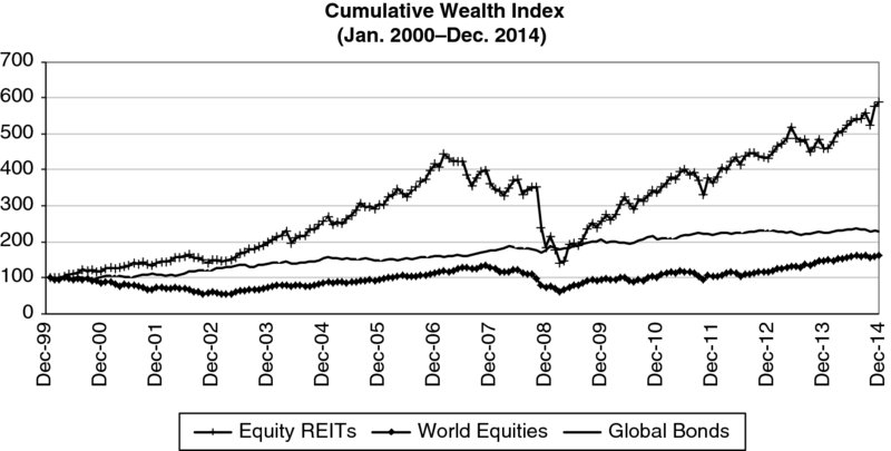
Exhibit 15.9B Cumulative Wealth
Exhibit 15.9C Betas and Correlations
| Multivariate Betas | World Equities | Global Bonds | U.S. High-Yield | Commodities | Annualized Estimated α | R2 |
| Equity REITs | 0.55** | 0.47** | 0.79** | −0.09 | 5.28% | 0.49** |
| Univariate | World | Global | U.S. High- | %Δ Credit | ||
| Betas | Equities | Bonds | Yield | Commodities | Spread | %Δ VIX |
| Equity REITs | 0.89** | 1.08** | 1.40** | 0.18** | −0.15** | −0.14** |
| World | Global | U.S. High- | %Δ Credit | |||
| Correlations | Equities | Bonds | Yield | Commodities | Spread | %Δ VIX |
| Equity REITs | 0.63** | 0.29** | 0.63** | 0.19** | −0.24** | −0.43** |
* = Significant at 90% confidence.
** = Significant at 95% confidence.

Exhibit 15.9D Scatter Plot of Returns
Exhibits 15.9c and 15.9d indicate historical correlations over the same time period. Exhibit 15.9c depicts high monthly return correlation between equity REITs and global equities as well as between equity REITs and U.S. high-yield bonds. However, the monthly return correlations were more modest between equity REITs and global bonds, changing credit spreads, and commodities. Note the substantial negative correlation of equity REITs with changes in the volatility index, indicating the tendency of equity REITs to perform poorly during periods of increasing uncertainty in equity market returns.
Exhibit 15.9d illustrates the correlation between equity REITs and world equities with a scatter plot. Note that the months with the very highest and lowest equity REIT returns corresponded to the months with similarly extreme world equity returns. These outlier months during extreme events can drive the estimated correlation.
Taken together, the empirics regarding the risk of equity REITs appear consistent with the high-risk nature of equity REITs that should be expected given the leverage utilized by REITs and the expectation that real estate values vary with the health of the overall economy. The historical average returns of equity REITs relative to world equity returns appear out of line with their systematic risks, and care should be taken in inferring that future average returns of equity REITs will remain so relatively high.
Review Questions
-
What is the complement option type to financial options?
-
What is the name of the point in a decision tree at which new information arrives?
-
List the two major approaches to valuing private commercial real estate equity.
-
Define effective gross income.
-
How does the numerator of a pre-tax discounting approach differ from the numerator of an after-tax discounting approach?
-
How does the equity residual approach to real estate valuation differ from a DCF approach applied to the assets of a real estate project?
-
What are the characteristics that distinguish syndications from other real estate investment vehicles?
-
A real estate project is estimated to offer a 10% after-tax rate of return when the depreciation allowed for tax purposes is equal to the true economic depreciation. In what direction would the expected rate of return change if the depreciation allowed for tax purposes were accelerated relative to the true economic depreciation, and why?
-
What is the effect of using appraised prices of real estate values to estimate risk when the appraisals are based on lagged information consisting of varying lengths of time lag?
-
What data (i.e., pieces of information) are required to construct a hedonic price index for real estate?