Chapter 8

The Supreme Law of Unreason

During the last 27 years of his life, which ended at the age of 78 in 1855, Carl Friedrich Gauss slept only once away from his home in Göttingen.1 Indeed, he had refused professorships and had declined honors from the most distinguished universities in Europe because of his distaste for travel.

Like many mathematicians before and after him, Gauss also was a childhood genius—a fact that displeased his father as much as it seems to have pleased his mother. His father was an uncouth laborer who despised the boy’s intellectual precocity and made life as difficult as possible for him. His mother struggled to protect him and to encourage his progress; Gauss remained deeply devoted to her for as long as she lived.

Gauss’s biographers supply all the usual stories of mathematical miracles at an age when most people can barely manage to divide 24 by 12. His memory for numbers was so enormous that he carried the logarithmic tables in his head, available on instant recall. At the age of eighteen, he made a discovery about the geometry of a seventeen-sided polygon; nothing like this had happened in mathematics since the days of the great Greek mathematicians 2,000 years earlier. His doctoral thesis, “A New Proof That Every Rational Integer Function of One Variable Can Be Resolved into Real Factors of the First or Second Degree,” is recognized by the cognoscenti as the fundamental theorem of algebra. The concept was not new, but the proof was.

Gauss’s fame as a mathematician made him a world-class celebrity. In 1807, as the French army was approaching Göttingen, Napoleon ordered his troops to spare the city because “the greatest mathematician of all times is living there.”2 That was gracious of the Emperor, but fame is a two-sided coin. When the French, flushed with victory, decided to levy punitive fines on the Germans, they demanded 2,000 francs from Gauss. That was the equivalent of $5,000 in today’s money and purchasing power—a heavy fine indeed for a university professor.a That was gracious of the Emperor, but fame is a two-sided coin. When the French, flushed with victory, decided to levy punitive fines on the Germans, they demanded 2,000 francs from Gauss. That was the equivalent of $5,000 in today’s money and purchasing power—a heavy fine indeed for a university professor.a A wealthy friend offered to help out, but Gauss rebuffed him. Before Gauss could say no a second time, the fine was paid for him by a distinguished French mathematician, Marquis Pierre Simon de Laplace (1749–1827). Laplace announced that he did this good deed because he considered Gauss, 29 years his junior, to be “the greatest mathematician in the world,”3 thereby ranking Gauss a few steps below Napoleon’s appraisal. Then an anonymous German admirer sent Gauss 1,000 francs to provide partial repayment to Laplace.

Laplace was a colorful personality who deserves a brief digression here; we shall encounter him again in Chapter 12.

Gauss had been exploring some of the same areas of probability theory that had occupied Laplace’s attention for many years. Like Gauss, Laplace had been a child prodigy in mathematics and had been fascinated by astronomy. But as we shall see, the resemblance ended there. Laplace’s professional life spanned the French Revolution, the Napoleonic era, and the restoration of the monarchy. It was a time that required unusual footwork for anyone with ambitions to rise to high places. Laplace was indeed ambitious, had nimble footwork, and did rise to high places.4

In 1784, the King made Laplace an examiner of the Royal Artillery, a post that paid a handsome salary. But under the Republic, Laplace lost no time in proclaiming his “inextinguishable hatred to royalty.”5 Almost immediately after Napoleon came to power, Laplace announced his enthusiastic support for the new leader, who gave him the portfolio of the Interior and the title of Count; having France’s most respected scientist on the staff added respectability to Napoleon’s fledgling government. But Napoleon, having decided to give Laplace’s job to his own brother, fired Laplace after only six weeks, observing, “He was a worse than mediocre administrator who searched everywhere for subtleties, and brought into the affairs of government the spirit of the infinitely small.”6 So much for academics who approach too close to the seats of power!

Later on, Laplace got his revenge. He had dedicated the 1812 edition of his magisterial Théorie analytique des probability to “Napoleon the Great,” but he deleted that dedication from the 1814 edition. Instead, he linked the shift in the political winds to the subject matter of his treatise: “The fall of empires which aspired to universal dominion,” he wrote, “could be predicted with very high probability by one versed in the calculus of chance.”7 Louis XVIII took appropriate note when he assumed the throne: Laplace became a Marquis.

Unlike Laplace, Gauss was reclusive and obsessively secretive. He refrained from publishing a vast quantity of important mathematical research—so much, in fact, that other mathematicians had to rediscover work that he had already completed. Moreover, his published work emphasized results rather than his methodology, often obliging mathematicians to search for the path to his conclusions. Eric Temple Bell, one of Gauss’s biographers, believes that mathematics might have been fifty years further along if Gauss had been more forthcoming; “Things buried for years or decades in [his] diary would have made half a dozen great reputations had they been published promptly.”8

Fame and secretiveness combined to make Gauss an incurable intellectual snob. Although his primary achievement was in the theory of numbers, the same area that had fascinated Fermat, he had little use for Fermat’s pioneering work. He brushed off Fermat’s Last Theorem, which had stood as a fascinating challenge to mathematicians for over a hundred years, as “An isolated proposition with very little interest for me, because I could easily lay down a multitude of such propositions, which one could neither prove nor dispose of.”9

This was not an empty boast. In 1801, at the age of 24, Gauss had published Disquisitiones Arithmeticae, written in elegant Latin, a trailblazing, historic work in the theory of numbers. Much of the book is obscure to a non-mathematician, but what he wrote was beautiful music to himself.10 He found “a magical charm” in number theory and enjoyed discovering and then proving the generality of relationships such as this:

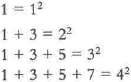
Or, in general, that the sum of the first n successive odd numbers is n². This would make the sum of the first 100 odd numbers, from 1 to 199, equal to 100², or 10,000; and the sum of the numbers from 1 to 999 would be equal to 250,000.

Gauss did deign to demonstrate that his theoretical work had important applications. In 1800, an Italian astronomer discovered a small new planet—technically, an asteroid—that he named Ceres. A year later Gauss set out to calculate its orbit; he had already calculated lunar tables that enabled people to figure out the date of Easter in any year. Gauss was motivated in large part by his desire to win a public reputation. But he also wanted to join his distinguished mathematical ancestors—from Ptolemy to Galileo and Newton—in research into celestial mechanics, quite aside from wishing to outdo the astronomical work of his contemporary and benefactor, Laplace. In any event, this particular problem was enticing in itself, given the paucity of relevant data and the speed with which Ceres rotated around the sun.

After a spell of feverish calculation, he came up with a precisely correct solution and was able to predict the exact location of Ceres at any moment. In the process he had developed enough skill in celestial mechanics to be able to calculate the orbit of a comet in just an hour or two, a task that took other scientists three or four days.

Gauss took special pride in his achievements in astronomy, feeling that he was following in the footsteps of Newton, his great hero. Given his admiration for Newton’s discoveries, he grew apoplectic at any reference to the story that the fall of an apple on Newton’s head had been the inspiration for discovering the law of gravity. Gauss characterized this fable as:

Silly! A stupid, officious man asked Newton how he discovered the law of gravitation. Seeing that he had to deal with a child intellect, and wanting to get rid of the bore, Newton answered that an apple fell and hit him on the nose. The man went away fully satisfied and completely enlightened.11

Gauss took a dim view of humanity in general, deplored the growing popularity of nationalist sentiments and the glories of war, and regarded foreign conquest as “incomprehensible madness.” His misanthropic attitudes may have been the reason why he stuck so close to home for so much of rfis life.12

Gauss had no particular interest in risk management as such. But he was attracted to the theoretical issues raised by the work in probability, large numbers, and sampling that Jacob Bernoulli had initiated and that had been carried forward by de Moivre and Bayes. Despite his lack of interest in risk management, his achievements in these areas are at the heart of modern techniques of risk control.

Gauss’s earliest attempts to deal with probability appeared in a book titled Theoria Motus (Theory of Motion), published in 1809, on the motion of heavenly bodies. In the book Gauss explained how to estimate an orbit based on the path that appeared most frequently over many separate observations. When Theoria Motus came to Laplace’s attention in 1810, he seized upon it with enthusiasm and set about clarifying most of the ambiguities that Gauss had failed to elucidate.

Gauss’s most valuable contribution to probability would come about as the result of work in a totally unrelated area, geodesic measurement, the use of the curvature of the earth to improve the accuracy of geographic measurements. Because the earth is round, the distance between two points on the surface differs from the distance between those two points as the crow flies. This variance is irrelevant for distances of a few miles, but it becomes significant for distances greater than about ten miles.

In 1816, Gauss was invited to conduct a geodesic survey of Bavaria and to link it to measurements already completed by others for Denmark and northern Germany. This task was probably little fun for an academic stick-in-the-mud like Gauss. He had to work outdoors on rugged terrain, trying to communicate with civil servants and others he considered beneath him intellectually—including fellow scientists. In the end, the study stretched into 1848 and tilled sixteen volumes when the results were published.

Since it is impossible to measure every square inch of the earth’s surface, geodesic measurement consists of making estimates based on sample distances within the area under study. As Gauss analyzed the distribution of these estimates, he observed that they varied widely, but, as the estimates increased in number, they seemed to cluster around a central point. That central point was the mean—statistical language for the average—of all the observations; the observations also distributed themselves into a symmetrical array on either side of the mean. The more measurements Gauss took, the clearer the picture became and the more it resembled the bell curve that de Moivre had come up with 83 years earlier.

The linkage between risk and measuring the curvature of the earth is closer than it might appear. Day after day Gauss took one geodesic measurement after another around the hills of Bavaria in an effort to estimate the curvature of the earth, until he had accumulated a great many measurements indeed. Just as we review past experience in making a judgment about the probability that matters will resolve themselves in the future in one direction rather than another, Gauss had to examine the patterns formed by his observations and make a judgment about how the curvature of the earth affected the distances between various points in Bavaria. He was able to determine the accuracy of his observations by seeing how they distributed themselves around the average of the total number of observations.

The questions he tried to answer were just variations on the kinds of question we ask when we are making a risky decision. On the average, how many showers can we expect in New York in April, and what are the odds that we can safely leave our raincoat at home if we go to New York for a week’s vacation? If we are going to drive across the country, what is the risk of having an automobile accident in the course of the 3,000-mile trip? What is the risk that the stock market will decline by more than 10% next year?

The structure Gauss developed for answering such questions is now so familiar to us that we seldom stop to consider where it came from. But without that structure, we would have no systematic method for deciding whether or not to take a certain risk or for evaluating the risks we face. We would be unable to determine the accuracy of the information in hand. We would have no way of estimating the probability that an event will occur—rain, the death of a man of 85, a 20% decline in the stock market, a Russian victory in the Davis Cup matches, a Democratic Congress, the failure of seatbelts, or the discovery of an oil well by a wildcatting firm.

The process begins with the bell curve, the main purpose of which is to indicate not accuracy but error. If every estimate we made were a precisely correct measurement of what we were measuring, that would be the end of the story. If every human being, elephant, orchid, and razor-billed auk were precisely like all the others of its species, life on this earth would be very different from what it is. But life is a collection of similarities rather than identities; no single observation is a perfect example of generality. By revealing the normal distribution, the bell curve transforms this jumble into order. Francis Galton, whom we will meet in the next chapter, rhapsodized over the normal distribution:

[T]he “Law Of Frequency Of Error”. . . reigns with serenity and in complete self-effacement amidst the wildest confusion. The huger the mob . . . the more perfect is its sway. Ft is the supreme law of Unreason. Whenever a large sample of chaotic elements are taken in hand . . . an unsuspected and most beautiful form of regularity proves to have been latent all along.13

Most of us first encountered the bell curve during our schooldays. The teacher would mark papers “on the curve” instead of grading them on an absolute basis—this is an A paper, this is a C+ paper. Average students would receive an average grade, such as B− or C+ or 80%. Poorer and better students would receive grades distributed symmetrically around the average grade. Even if all the papers were excellent or all were terrible, the best of the lot would receive an A and the worst a D, with most grades falling in between.

Many natural phenomena, such as the heights of a group of people or the lengths of their middle fingers, fall into a normal distribution. As Galton suggested, two conditions are necessary for observations to be distributed normally, or symmetrically, around their average. First, there must be as large a number of observations as possible. Second, the observations must be independent, like rolls of the dice. Order is impossible to find unless disorder is there first.

People can make serious mistakes by sampling data that are not independent. In 1936, a now-defunct magazine called the Literary Digest took a straw vote to predict the outcome of the forthcoming presidential election between Franklin Roosevelt and Alfred Landon. The magazine sent about ten million ballots in the form of returnable postcards to names selected from telephone directories and automobile registrations. A high proportion of the ballots were returned, with 59% favoring Landon and 41% favoring Roosevelt. On Election Day, Landon won 39% of the vote and Roosevelt won 61%. People who had telephones and drove automobiles in the mid-1930s hardly constituted a random sample of American voters: their voting preferences were all conditioned by an environment that the mass of people at that time could not afford.

Observations that are truly independent provide a great deal of useful information about probabilities. Take rolls of the dice as an example.

Each of the six sides of a die has an equal chance of coming up. If we plotted a graph showing the probability that each number would appear on a single toss of a die, we would have a horizontal line set at one-sixth for each of the six sides. That graph would bear absolutely no resemblance to a normal curve, nor would a sample of one throw tell us anything about the die except that it had a particular number imprinted on it. We would be like one of the blind men feeling the elephant.

Now let us throw the die six times and see what happens. (I asked my computer to do this for me, to be certain that the numbers were random.) The first trial of six throws produced four 5s, one 6, and one 4, for an average of exactly 5.0. The second was another hodgepodge, with three 6s, two 4s, and one 2, for an average of 4.7. Not much information there.

After ten trials of six throws each, the averages of the six throws began to cluster around 3.5, which happens to be the average of 1+2+3+4+5+6, or the six faces of the die—and precisely half of the mathematical expectation of throwing two dice. Six of my averages were below 3.5 and four were above. A second set of ten trials was a mixed bag: three of them averaged below 3.0 and four averaged above 4.0; there was one reading each above 4.5 and below 2.5.

The next step in the experiment was to figure the averages of the first ten trials of six throws each. Although each of those ten trials had an unusual distribution, the average of the averages came to 3.48! The average was reassuring, but the standard deviation, at 0.82, was wider than I would have liked.b In other words, seven of the ten trials fell between 3.48 + 0.82 and 3.48 − 0.82, or between 4.30 and 2.66; the rest were further away from the average.

Now I commanded the computer to simulate 256 trials of six throws each. The first 256 trials generated an average almost on target, at 3.49; with the standard deviation now down to 0.69, two-thirds of the trials were between 4.18 and 2.80. Only 10% of the trials averaged below 2.5 or above 4.5, while more than half landed between 3.0 and 4.0.

The computer still whirling, the 256 trials were repeated ten times. When those ten samples of 256 trials each were averaged, the grand average came out to 3.499. (I carry out the result to three decimal places to demonstrate how close I came to exactly 3.5.) But the impressive change was the reduction of the standard deviation to only 0.044. Thus, seven of the ten samples of 256 trials fell between the narrow range of 3.455 and 3.543. Five were below 3.5 and five were above. Close to perfection.

Quantity matters, as Jacob Bernoulli had discovered. This particular version of his insight—the discovery that averages of averages miraculously reduce the dispersion around the grand average—is known as the central limit theorem. This theorem was first set forth by Laplace in 1809, in a work he had completed and published just before he came upon Gauss’s Theoria Motus in 1810.

Averages of averages reveal something even more interesting. We began the experiment I have just described with a die with, as usual, six faces, each of which had an equal chance of coming up when we threw it. The distribution then was flat, bearing no likeness at all to a normal distribution. As the computer threw the die over and over and over, accumulating a growing number of samples, we gleaned more and more information about the die’s characteristics.

Very few of the averages of six throws came out near one or six; many of them fell between two and three or between four and five. This structure is precisely what Cardano worked out for his gambling friends, some 250 yean ago, as he groped his way toward the laws of chance. Many throws of a single die will average out at 3.5. Therefore, many throws of two dice will average out at double 3.5, or .7.0. As Cardano demonstrated, the numbers on either side of 7 will appear with uniformly diminishing frequency as we move away from 7 to the limits of 2 and 12.

The normal distribution forms the core of most systems of risk management. The normal distribution is what the insurance business is all about, because a fire in Chicago will not be caused by a fire in Atlanta, and the death of one individual at one moment in one place has no relationship to the death of another individual at another moment in a different place. As insurance companies sample the experience of millions of individuals of different ages and of each gender, life expectancies begin to distribute themselves into a normal curve. Consequently, life insurance companies can come up with reliable estimates of life expectancies for each group. They can estimate not only average life expectancies but also the ranges within which actual experience is likely to vary from year to year. By refining those estimates with additional data, such as medical histories, smoking habits, domicile, and occupational activities, the companies can establish even more accurate estimates of life expectancies.c

On occasion, the normal distribution provides even more important information than just a measure of the reliability of samples. A normal distribution is most unlikely, although not impossible, when the observations are dependent upon one another—that is, when the probability of one event is determined by a preceding event. The observations will fail to distribute themselves symmetrically around the mean.

In such cases, we can profitably reason backwards. If independence is the necessary condition for a normal distribution, we can assume that evidence that distributes itself into a bell curve comes from observations that are independent of one another. Now we can begin to ask some interesting questions.

How closely do changes in the prices of stocks resemble a normal distribution? Some authorities on market behavior insist that stock prices follow a random walk—that they resemble the aimless and unplanned lurches of a drunk trying to grab hold of a lamppost. They believe that stock prices have no more memory than a roulette wheel or a pair of dice, and that each observation is independent of the preceding observation. Today’s price move will be whatever it is going to be, regardless of what happened a minute ago, yesterday, the day before, or the day before that.

The best way to determine whether changes in stock prices are in fact independent is to find out whether they fall into a normal distribution. Impressive evidence exists to support the case that changes in stock prices are normally distributed. That should come as no surprise. In capital markets as fluid and as competitive as ours, where each investor is trying to outsmart all the others, new information is rapidly reflected in the price of stocks. If General Motors posts disappointing earnings or if Merck announces a major new drug, stock prices do not stand still while investors contemplate the news. No investor can afford to wait for others to act first. So they tend to act in a pack, immediately moving the price of General Motors or Merck to a level that reflects this new information. But new information arrives in random fashion. Consequently, stock prices move in unpredictable ways.

Interesting evidence in support of this view was reported during the 1950s by Harry Roberts, a professor at the University of Chicago.14 Roberts drew random numbers by computer from a series that had the same average and the same standard deviation as price changes in the stock market. He then drew a chart showing the sequential changes of those random numbers. The results produced patterns that were identical to those that stock-market analysts depend on when they are trying to predict where the market is headed. The real price movements and the computer-generated random numbers were indistinguishable from each other. Perhaps it is true that stock prices have no memory.

The accompanying charts show monthly, quarterly, and annual percentage changes in the Standard & Poor’s Index of 500 stocks, the professional investor’s favorite index of the stock market. The data run from January 1926 through December 1995, for 840 monthly observations, 280 quarterly observations, and 70 annual observations.d

Although the charts differ from one another, they have two features in common. First, as J.P. Morgan is reputed to have said, “The market will fluctuate.” The stock market is a volatile place, where a lot can happen in either direction, upward or downward. Second, more observations fall to the right of zero than to the left: the stock market has gone up, on the average, more than it has gone down.

The normal distribution provides a more rigorous test of the random-walk hypothesis. But one qualification is important. Even if the random walk is a valid description of reality in the stock market—even if changes in stock prices fall into a perfect normal distribution—the mean will be something different from zero. The upward bias should come as no surprise. The wealth of owners of common stocks has risen over the long run as the economy and the revenues and profits of corporations have grown. Since more stock-price movements have been up than down, the average change in stock prices should work out to more than zero.

In fact, the average increase in stock prices (excluding dividend income) was 7.7% a year. The standard deviation was 19.3%; if the future will resemble the past, this means that two-thirds of the time stock prices in any one year are likely to move within a range of +27.0% and −12.1%. Although only 2.5% of the years—one out of forty—are likely to result in price changes greater than +46.4%, there is some comfort in finding that only 2.5% of the years will produce bear markets worse than −31.6%.

Stock prices went up in 47 of the 70 years in this particular sample of history, or in two out of every three years. That still leaves stocks falling in 23 of those years; and in 10 of those 23 years, or nearly half, prices plummeted by more than one standard deviation—by more than 12.1%. Indeed, losses in those 22 bad years averaged −15.2%.

Note that the three charts have different scales. The number of observations, shown on the vertical scales, will obviously differ from one another—in any given time span, there are more months than quarters and more quarters than years. The horizontal scales, which measure the range of outcomes, also differ, because stock prices move over a wider span in a year than in a quarter and over a wider span in a quarter than during a month. Each number on the horizontal scale measures price changes between the number to the left and that number.

Let us look first at the 840 monthly changes. The mean monthly change was +0.6%. If we deduct 0.6% from each of the observations in order to correct for the natural upward bias of the stock market over time, the average change becomes +0.00000000000000002%, with 50.6% of the months plus and 49.4% of the months minus. The first quartile observation, 204 below the mid-point, was −2.78%; the third quartile observation, 204 above the mid-point, was +2.91. The symmetry of a normal distribution appears to be almost flawless.

The random character of the monthly changes is also revealed by the small number of runs—of months in which the stock market moved in the same direction as in the preceding month. A movement in the same direction for two months at a time occurred only half the time; runs as long as five months occurred just 9% of the time.

The chart of monthly changes does have a remarkable resemblance to a normal curve. But note the small number of large changes at the edges of the chart. A normal curve would not have those untidy bulges.

Now look at the chart of 280 quarterly observations. This chart also resembles a normal curve. Nevertheless, the dispersion is wide and, once again, those nasty outliers pop up at the extremes. The 1930s had two quarters in which stock prices fell by more than a third—and two quarters in which stock prices rose by nearly 90%! Life has become more peaceful since those woolly days. The quarterly extremes since the end of the Second World War have been in the range of +25% and −25%.

The average quarterly change is +2.0%, but the standard deviation of 12.1% tells us that +2.0% is hardly typical of what we can expect from quarter to quarter. Forty-five percent of the quarters were less than the average of 2.0%, while 55% were above the quarterly average.

The chart of 70 annual observations is the neatest of the three, but the scaling on the horizontal axis of the chart, which is four times the size of the scaling on the quarterly chart, bunches up a lot of large changes.

The differences in scales are not just a technical convenience to make the different time periods comparable to one another on these three charts. The scales tell an important story. An investor who bought and held a portfolio of stocks for 70 years would have come out just fine. An investor who had expected to make a 2% gain each and every three-month period would have been a fool. (Note that I am using the past tense here; we have no assurance that the past record of the stock market will define its future.)

So the stock-market record has produced some kind of resemblance to a random walk, at least on the basis of these 840 monthly observations, because data would not appear to be distributed in this manner around the mean if stock-price changes were not independent of one another—like throws of the dice. After correction for the upward drift, changes were about as likely to be downward as upward; sequential changes of more than a month or so at a time were rare; the volatility ratios across time came remarkably close to what theory stipulates they should have been.

Assuming that we can employ Jacob Bernoulli’s constraint that the future will look like the past, we can use this information to calculate the risk that stock prices will move by some stated amount in any one month. The mean monthly price change in the S&P table was 0.6% with a standard deviation of 5.8%. If price changes are randomly distributed, there is a 68% chance that prices in any one month will change by no less than −5.2% or by no more than +6.4%. Suppose we want to know the probability that prices will decline in any one month. The answer works out to 45%—or a little less than half the time. But a decline of more than 10% in any one month has a probability of only 3.5%, which means that it is likely to happen only about once every thirty months; moves of 10% in either direction will show up about once in every fifteen months.

As it happens, 33 of the 840 monthly observations, or about 4% of the total, were more than two standard deviations away from the monthly average of +0.6%—that is, worse than −11% and greater than 12.2%. Although 33 superswings are fewer than we might expect in a perfectly random series of observations, 21 of them were on the downside; chance would put that number at 16 or 17. A market with a built-in long-term upward trend should have even fewer disasters than 16 or 17 over 816 months.

At the extremes, the market is not a random walk. At the extremes, the market is more likely to destroy fortunes than to create them. The stock market is a risky place.

Up to this point, our story has been pretty much about numbers. Mathematicians have held center stage as we studied the innovations of ancient Hindus, Arabs, and Greeks all the way up to Gauss and Laplace in the nineteenth century. Probability rather than uncertainty has been our main theme.

Now the scene is about to shift. Real life is not like Paccioli’s game of balla, a sequence of independent or unrelated events. The stock market looks a lot like a random walk, but the resemblance is less than perfect. Averages are useful guides on some occasions but misleading on many others. On still other occasions numbers are no help at all and we are obliged to creep into the future guided only by guesses.

This does not mean that numbers are useless in real life. The trick is to develop a sense of when they are relevant and when they are not. So we now have a whole new set of questions to answer.

For instance, which defines the risk of being hit by a bomb, seven million people or one elephant? Which of the following averages should we use to define the stock market’s normal performance: the average monthly price change of +0.6% from 1926 to 1995, the piddling average of only +0.1% a month from 1930 to 1940, or the enticing average of +1.0% a month from 1954 to 1964?

In other words, what do we mean by “normal”? How well does any particular average describe normal? How stable, how powerful, is an average as an indicator of behavior? When observations wander away from the average of the past, how likely are they to regress to that average in the future? And if they do regress, do they stop at the average or overshoot it?

What about those rare occasions when the stock market goes up five months in a row? Is it true that everything that goes up must come down? Doth pride always goeth before a fall? What is the likelihood that a company in trouble will bring its affairs into order? Will a manic personality swing over to depression any time soon, and vice versa? When is the drought going to end? Is prosperity just around the corner?

The answers to all these questions depend on the ability to distinguish between normal and abnormal. Much risk-taking rests on the opportunities that develop from deviations from normal. When analysts tell us that their favorite stock is “undervalued,” they are saying that an investor can profit by buying the stock now and waiting for its value to return to normal. On the other hand, mental depressions or manic states sometimes last a lifetime. And the economy in 1932 refused to move itself around the corner, even though Mr. Hoover and his advisers were convinced that prodding by the government would only deter it from finding its way back all by itself.

Nobody actually discovered the concept of “normal” any more than anybody actually discovered the concept of “average.” But Francis Galton, an amateur scientist in Victorian England, took the foundation that Gauss and his predecessors had created to support the concept of average—the normal distribution—and raised a new structure to help people distinguish between measurable risk and the kind of uncertainty that obliges us to guess what the future will bring.

Galton was not a scientist in search of immutable truths. He was a practical man, enthusiastic about science but still an amateur. Yet his innovations and achievements have had a lasting impact on both mathematics and hands-on decision-making in the everyday world.

a The franc/dollar exchange rate has been remarkably steady over the years at around 5:1. Hence, 2,000 francs was the equivalent of $400 dollars of 1807 purchasing power. A dollar in 1807 bought about twelve times as much as today’s dollar.

b The standard deviation was the device that de Moivre discovered for measuring the dispersion of observations around their mean. Approximately two-thirds of the observations (68.26%) will fall within a range of plus or minus one standard deviation around the mean; 95.46% will fall within two standard deviations around the mean.

c Richard Price’s experience reminds us that the data themselves must be of good quality. Otherwise, GIGO: garbage in, garbage out.

d Readers skilled in statistics will protest that I should have used the lognormal analysis in the discussion that follows. For readers not so skilled, the presentation in this form is much more intelligible and the loss of accuracy struck me as too modest to justify further complexity.

Notes

1. The biographical material on Gauss is primarily from Shaaf, 1964, and from Bell, 1965.

2. Schaaf, 1964, p. 40.

3. Bell, 1965, p. 310.

4. The biographical background on Laplace is from Newman, 1988d, pp. 1291–1299.

5. Newman, 1988d, p. 1297.

6. Ibid., p. 1297.

7. Ibid., p. 1297.

8. Bell, 1965, p. 324.

9. Ibid., p. 307.

10. The following discussion and examples are from Schaaf, 1964, pp. 23–25.

11. Bell, 1965, p. 321.

12. Ibid., p. 331.

13. Quoted in Schaaf, 1964, p. 114.

14. Details on Roberts’ experiment may be found in Bernstein, 1992, pp. 98–103.