Although you can light a 3D scene with basic lights and shadows to create a render that looks realistic, there are advanced lighting and rendering systems that take the realism much further. These systems pay close attention to the physical realities of light and how it interacts with our environments.
This chapter includes the following critical information:
•Overview of scanline and ray trace rendering
•Overview of PBR systems and their unique features
•Introduction to render passes and AOVs
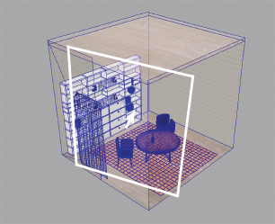
“An image rendered using path tracing, demonstrating notable features of the technique.” by Qutorial licensed via Creative Commons Attribution-ShareAlike 4.0 International (CC BY-SA 4.0).
In this book, I use the terms PBR and Physically Based Rendering to refer to 3D lighting systems, 3D shaders, and 3D rendering systems that strive for physical accuracy in order to create renders that look photoreal or that approach photorealism. When you light a 3D scene, PBR may be an option. However, there are several considerations to take into account:
Is physical accuracy in your lighting necessary? If the scene you are lighting does not benefit from light bounce, color bleed, or accurate shadow decay, then it might not be necessary to use PBR. This decision may be based on aesthetic criteria alone—for example, if the lighting project is stylistic, then it might not require excessive realism.
Can you achieve a realistic look without a PBR system? It’s possible to use non-PBR shaders, lights, and rendering systems to light a scene and produce a render that looks fairly realistic. Such a set up may never achieve the degree of realism of a PBR render, but it may be aesthetically suitable for some projects. (Note that the 3D scenes featured in earlier chapters did not employ PBR.)
Does your lighting schedule allow you enough time to use PBR? In general, PBR systems take more time to set up, adjust, and render than non-PBR systems.
Note that rendering systems, as a term, refers to a specific approach to rendering that uses particular algorithms. An algorithm is a set of rules followed during problem-solving operations. Renderers refer to specific rendering systems provided by software companies.
Before discussing PBR in more detail, it pays to be familiar with two of the most common rendering systems: scanline and ray tracing. Note that all the rendering systems are dependent on rasterization, whereby 2D shapes are converted to raster images, which are composed of rows of pixels (scanlines). With a 3D program, 3D polygonal shapes are converted to 2D via the view plane of the 3D camera.
A scanline rendering system works on a row-by-row basis. For each scanline, the system follows these basic steps:
1.Identify intersections between polygon edges and the current scanline (Figure 5.1).
2.Sort the intersections along the scanline from left to right.
3.Fill in all pixels between pairs of intersections.
Figure 5.1 A simplified representation of a scanline rendering system. A scanline is shown in red. A polygon shape, flattened into 2D by the camera’s view plane, is colored gray. Edge intersections are indicated with white dots. Filled in pixels are drawn as yellow dots.
Scanline rendering systems determine the color of the fill area by taking into account the properties of the shader assigned to the polygon and any present lights and shadows. Some 3D programs offer a scanline renderer as an option. For example, Autodesk Maya, Autodesk 3ds Max, and Blender include optional scanline renderers. Scanline functions may be included as a base component of advanced renderers. For example, you can force mental ray to scanline render and forgo ray tracing.
A scanline rendering system is very efficient. However, the systems have the following limitations:
•No reflections
•No transmissions / refractions
•Creates approximated specular highlights instead of specular reflections
For example, in Figure 5.2, a transparent surface is rendered with a scanline renderer but appears like thin plastic due to the lack of proper reflections or refractions.
Figure 5.2 Left: An ornate bottle is rendered with a scanline renderer. Right: The same bottle is given 100 percent transparency through the assigned Blinn shader. The resulting bottle appears like thin plastic due to the lack of reflections or refractions. Note that the depth map shadow also fails to take into account the transparency.
As discussed in Chapter 3, ray tracing rendering systems trace rays through a scene (Figure 5.3). The rays reflect off the surfaces, transmit through surfaces, or are absorbed by the surfaces (the ray is killed off). Ray tracing systems are able to offer the following:
•Absorption (light rays have a limited number of bounces)
These features, in and of themselves, do not create a PBR render. However, ray tracing is often a critical component of PBR rendering systems. Ray tracing systems may require a great deal of processor time due to the potentially high number of light rays and ray/surface intersections. As such, the systems generally offer controls for limiting the number of times an individual ray is permitted to reflect or transmit.
Figure 5.3 A simplified representation of ray trace rendering. The brightness of a surface point is determined by comparing the vector between the camera and surface point to the vector between the surface point and the light.
Graphic by Henrik, licensed under the Creative Commons Attribution-ShareAlike 4.0 International (CC BY-SA 4.0).
Figure 5.4 Left: Bottle rendered with a ray trace renderer and ray trace shadows, allowing for reflections, refractions, and semitransparent shadows. Right: Same bottle with 75 percent transparency, allowing the purple diffuse color to show. Note that the specular highlights generated by the Blinn shader are only approximations of specular reflections of light sources.
Here are a few things to keep in mind when it comes to PBR shaders, PBR lighting systems, and PBR rendering systems/renderers:
•Linear Calculations For a PBR renderer to function in a physically accurate way, it must operate in a linear color space (a color space with no gamma correction). As such, texture bitmaps with sRGB color space must be converted to linear color space. If color space management tools are provided by a 3D program, there will be an opportunity to interpret the color space of imported bitmaps. See Chapter 3 for more information on linear color space and color space management.
•Shader Properties A PBR shader may support all of the properties listed at the start of this section. PBR shaders are often used by video game engines, requiring the use of specially prepared PBR texture bitmaps. The maps may cover such properties as albedo (diffuse color without lighting), metalness (metallic specularity), glossiness/roughness (degree of diffusion for reflections), and AO (Ambient Occlusion)/micro-occlusions (light absorption in nooks and crannies). One hallmark of a PBR shader is the ability to create specular reflections of light sources. For example, in Figure 5.5, a PBR shader is assigned to the bottle and ground plane. Note that the shaders discussed here are sometimes said to use PBS (Physically Based Shading).
Figure 5.5 The bottle and ground plane are assigned to PBR shaders. The specular highlights become more accurate specular reflections of the lights in the scene. Even though the point lights do not have a specific width in world space, both non-PBR and PBR shaders recognize the different intensities of the lights when calculating the specular highlights/specular reflections.
•Lighting Requirements PBR lighting systems may not require PBR shaders to function. As long as the shaders have basic properties such as diffuse color and reflectivity, the lighting systems will generally work (although some shader functions, like bump mapping, may be ignored). That said, PBR shaders will provide more accurate results for PBR lighting and rendering systems.
•Renderer Requirements PBR rendering systems may not require PBR shaders or PBR-based lights to function. That said, PBR shaders and PBR-based lights will provide more accurate results. For example, area lights are more physically accurate than 0-width point lights or non-positional ambient lights.
•Light Variations Some PBR renderers provide their own light variations, such as specialized area lights or spot lights. In general, these are not required to make the PBR setup function; however, such lights often include additional properties to increase the accuracy of the resulting PBR render.
Microfacets are tiny surface imperfections. When randomly oriented, microfacets create diffuse, matte-like surfaces that create non-glossy reflections. When oriented in the same directions, microfacets create glossy, coherent, mirror-like reflections. Fresnel reflectivity alters the strength of the reflection based on the viewing angle. Metallic specularity bases the color of the specular reflection on the diffuse color. Non-metallic specularity bases the specular reflection color or the color of the incoming light ray. BRDF undertakes energy conservation by ensuring that the light energy reflected off a surface is equal to or less than the energy carried by the incident light ray. For more detail on these shader properties, see the sections “3D Light Interaction with Shaders” and “Common Shader Properties” in Chapter 3.
In this section, we’ll review common rendering and lighting systems that use PBR. This is by no means an exhaustive list, but it does include systems that are commonly used. Each system has strengths and weaknesses, which are discussed here.
GI (Global Illumination), as a term, has come to refer to any rendering system that simulates light bounce (more accurately known as indirect illumination, intersurface reflections, or secondary diffuse illumination). There are several forms of GI that are available:
Photon mapping This form of GI emits virtual photons from lights and traces the photons as they bounce through the scene. Based on shader qualities, photons reflect off surfaces, transmit through surfaces, or are absorbed (killed off). Photon mapping follows BRDF by altering the energies of reflected and transmitted photons. The energies are stored as red, green, and blue color values; hence, the resulting secondary diffuse illumination takes on the color of encountered surfaces and color bleed occurs. Secondary surface intersections and photon energies are stored in special photon maps. The maps are combined with more traditional scanline and ray trace renderers to create the final image. Photon mapping can be time-intensive due to the large number of photons that need to be traced through the scene. Photon mapping may also suffer from a graininess as the photon intersections must be averaged and each intersection may cover a fairly small area in world space (although the radius of photon intersections is generally adjustable). Hence, photon mapping is often combined with final gather. A simple example of photon mapping is demonstrated by Figure 5.6.
As a more complex example of photon mapping, we can return to the interior model we lit in Chapter 4. Instead of using two area lights, we can employ a single area light placed within the window area (Figure 5.7). All of the secondary diffuse illumination comes courtesy of the photon mapping.
Photon mapping is often used to generate caustics, which are focused specular highlights created by reflection or refraction. Caustics are often seen when light refracts through or reflects off glass, crystal, water, or shiny metal (Figure 5.8).
“A rainbow is the product of physics working for your appreciation of beauty”—Kyle Hill
Figure 5.6 Left: A cyan plane hovers over a gray plane, lit by a point light. Middle: GI with photon mapping is activated. The cyan dots on the lower plane are produced by photon intersections. The photons are generated by the point light and bounce off the surfaces in the scene. The diffuse color of the surfaces the photons bounce off affects the photon color and intensity. The photon count, in this case, is too low and the photon intersections do not blend smoothly. Right: The photon count is increased and the radius of the photon intersections is adjusted until the photon contribution blends smoothly, forming cyan light bounce on the gray plane.Figure 5.7 The interior room is rendered with photon mapping. A single area light, placed just beyond the left side of frame, is set to emit a total of 75,000 photons. In general, the higher the photon count, the more accurate the render but the longer the render times.Figure 5.8 Bright white caustic rings created with photon mapping and final gather.
Wine glass model by Mig91.
Final gather You can use this GI system, also known as final gathering, by itself or in conjunction with another GI system, such as photon mapping. Final gather calculates light contribution by creating final gather points where a camera view ray (also known as an eye ray) intersects a surface. The final gather point sends out secondary final gather rays in a hemispherical cloud (Figure 5.9). If the final gather rays encounter other surfaces, then the light intensities of the encountered surfaces are averaged with the intensity of the original intersection point. Much like ray tracing, final gather offers a means to limit the number of bounces a secondary ray is permitted. It’s also possible to limit the distance the final gather rays travel through the scene. When compared to photon mapping, final gather tends to produce smoother results with less set up time and render time. However, the light bleed created by final gather tends to be more subtle than the bleed produced by photon mapping (Figure 5.10). Final gather is provided by renderers such as mental ray and is available in programs that include Maya, 3ds Max, AutoCAD, and Unity.
Figure 5.9 A simplified representation of the final gather process. The cyan dot represents potential color bleed.Figure 5.10 The cyan plane is rendered with final gather. Compare this to the photon mapping render in Figure 5.6 earlier in this section.
Radiosity This type of GI calculates the intensity (brightness) of all surfaces in the 3D scene. The system does this by determining the amount of light reflected off each surface and how much of that light reaches every other surface (Figure 5.11). The results are stored by each unit of each surface, where each surface is broken into smaller units (sometimes called patches or elements, these do not necessarily follow the polygon face layout). The radiosity information is combined with the output of other render systems, such as ray tracing (Figure 5.12). Radiosity is view-independent and not reliant on a particular camera setup. However, conventional radiosity systems are unable to take into account specular reflectivity or transparency. In addition, the system is dependent on the number of units that the surfaces have been divided into and can suffer from graininess of poorly-defined shadow areas. However, recent developments of radiosity systems have optimized the process, making radiosity more viable. Programs such as 3ds Max and renderers such as Pixar RenderMan continue to support radiosity.
Figure 5.11 A simplified representation of the radiosity process. The dots represent light bounce.
Point cloud This form of GI approximates light bounce by creating a point cloud out of all the geometry in the scene. The point cloud simplifies the scene by only including a limited number of micropolygons. Each micropolygon is approximated with a disc. The system tests for disc intersections to determine if there are intersurface reflections. Hence, ray tracing is not needed to determine those reflections. Point cloud GI is currently available with RenderMan and 3Delight renderers.
Figure 5.12 Left: A render without radiosity. Right: A render with radiosity. Note the color bleed on the floor plane as well as the rim lighting created by light bouncing off the background wall.
Left image: “Renderbild ohne Radiosity” by Loebek licensed via Creative Commons Attribution-ShareAlike 3.0 Unported (CC BY-SA 3.0). Right image: “Raytracing Image mit Radiosity” by Loebek licensed via Creative Commons Attribution-ShareAlike 3.0 Unported (CC BY-SA 3.0).
Irradiance cache Another GI approximation that uses a sparse representation of surfaces visible to the camera to reduce the number of surface intersections necessary to calculate light bounce. The system assumes that the secondary illumination changes gradually over flat surfaces and that those surfaces require fewer GI calculations. Irradiance caches are available to such 3D programs as Cinema 4D and 3D renderers such as Redshift. Irradiance, in this case, refers to the amount of light energy a surface receives.
Path tracing / Monte Carlo ray tracing This form of ray tracing is considered the most physically accurate 3D rendering method at the time of writing. It is able to generate soft shadows, depth of field, motion blur, caustics, indirect illumination, and ambient occlusion without specialized shaders or post-processing steps. (Ambient occlusion calculates how any given point on a surface is exposed to ambient light.) As such, the use of path tracing supplants the need to employ GI systems such as final gather or photon mapping. The opening figure for this chapter was created with path tracing. In Figure 5.13, the room model is rendered with path tracing. The location of a single area light is indicated by Figure 5.14. As an additional example, the lamp scene first seen in Chapter 4 is revised with a path tracing renderer (Figure 5.15). The point light serving as fill is deleted and the two spot lights are left in their original positions. The spot light decays are set to linear and the light intensities are increased. The shadows are switched from standard ray trace to path-tracing supported shadows provided by the renderer.
Path tracing is built on the following principles:
1)In an indoor setting, all surfaces contribute illumination to all other surfaces.
2)Light emitted from a light source and reflected from a surface is considered the same.
3)Reflected light scatters in a way related to the incident angle of the arriving illumination.
Along with these principles is the assumption that “everything is shiny”—that is, all surfaces offer some degree of specular reflectivity and that no surface is 100 percent diffuse. As such, path tracing renderers do not rely on the reflectivity properties of non-PBR shaders. Instead, path tracing uses specular properties and creates specular reflections that accurately take into account the size, shape, and intensity of light sources.
These principles place some limitations on path tracing. For example, path tracing may not produce accurate subsurface scattering or incandescence. However, recent iterations of path tracing renderers have overcome many of the limitations. Path tracing serves as the core for the Arnold, Octane Render, Blender Cycles, and Corona renderers.
Figure 5.13 The interior room is rendered with a path tracing renderer. With path tracing, a single area light is required with no need of additional fill lights. Note that the specular reflections, seen on the edge of the table and on the face of the vase, reveal the rectangular shape of the area light. The light is set to cast shadows. In general, path tracing takes significantly more time to render than a standard ray tracing renderer.Figure 5.14 Approximate location of the key area light. Additional walls and a ceiling are added to present additional surfaces for light bounce. A vertical opening is left as a virtual window for the light to pass through.
“Color is my day-long obsession, joy and torment.”—Claude Monet
Figure 5.15 The lamp scene is rendered with path tracing. A fill light is not necessary. Note the more accurate specular reflections in the lamp base and on the various objects on the table. Also note the shadow decay over distance; where the shadow is distant from the shadow-casting object, it is soft.
IBL (Image-Based Lighting) is a 3D lighting system that uses a bitmap image to determine light intensity and color with the aid of a spherical projection (see Figure 3.22 in Chapter 3 of an example of the projection sphere). Because IBL relies on an image to determine lighting information, it’s often used for visual effects, architectural visualization, and other areas where it’s necessary to replicate a real-world location accurately. In fact, the images are usually sourced from digital photos of real locations. As such, photos used for IBL are often HDR (High-Dynamic Range). HDR photos combine multiple exposures within a single image with a high bit-depth, floating-point accuracy to ensure that all parts of the image are properly exposed. LDR (Low-Dynamic Range) images, such as an 8-bit PNG or Targa, are unable to store such large value ranges. Nevertheless, you can use an LDR image with IBL. For example, in Figure 5.16, an IBL setup is used to light the bottle and ground plane. Note that the image mapped to the IBL sphere appears in the background unless you adjust the IBL sphere visibility. The IBL image also appears in reflections.
Figure 5.16 Left: The bottle and ground plane are assigned to a non-reflective shader. The light color, light intensity, and soft, overlapping shadows are generated by an IBL system using the image featured in Figure 5.17. Right: The same bottle is assigned to a reflective shader. The IBL system provides the reflections.
Because the IBL projection is spherical, it requires an image with a special mapping. Equirectangular (also known as spherical or lat/long) mappings are common as 360 virtual reality cameras are able to produce photos with that mapping (Figure 5.17). However, IBL systems may also accept probe/angular style mappings (which appear like a reflection in chrome ball) or cubic crosses (where six views are unfolded into a cross-like pattern). The IBL sphere essentially shoots directional light rays from the sphere surface to the center of the sphere; the light color and relative intensity of each ray is taken from the nearest pixel of the mapped image.
Figure 5.17 An equirectangular-mapped photo of a back yard from the view of an iron bench. Although this is an LDR image, it was used to light the model in Figure 5.16. This image is included as 360casa.png in the Textures folder included with the exercise files.
Some 3D programs and 3D renderers provide a complete sky lighting system that emulates outdoor, sun-lit lighting. With these systems, the lighter is able to select the angle of the sun to mimic a particular time of day, choose a sun intensity, and set the sun color. The color of the empty 3D space is altered to match the sun color and thus create a sky. To add light bounce, you can combine the sky system with other GI systems. For example, Figure 5.18 features renders created with mental ray’s Physical Sun & Sky system in combination with final gather. As for other programs and renderers, 3ds Max includes Sunlight and Daylight lighting systems. The Arnold renderer offers a sky shader. Next Limit Technologies Maxwell Render, Glare Technologies Indigo, and V-Ray renderers offer their own sun and sky systems.
Figure 5.18 Top: Building lit with mental ray’s Physical Sun & Sky system. The direction of the virtual sun is indicated by the arrows. Bottom: Same system with the lower sun angle and a sun color shifted towards red. The light bounce is provided by a final gather.
The following list highlights advanced 3D renderers that support various PBR functions. This is by no means a complete list. Advances in 3D rendering occur fairly swiftly, so this list will no doubt evolve over the years following the book’s publication. These renderers are available as plug-ins for a wide range of popular 3D programs.
3Delight (www.3delight.com) Supports path tracing and non-tracing rendering techniques and is based on the RenderMan rendering standard.
Arnold (Solid Angle, www.solidangle.com) Uses path tracing while supporting fur, hair, SSS, volumetric effects, custom channel render passes, and geometry instancing.
Corona (Render Legion s.r.o., corona-renderer.com) Uses path tracing, but supports “reality hacks” to override PBR functions and make the renderer more efficient.
Indigo (Glare Technologies, www.indigorenderer.com) Supports SSS, volumetric effects, photometric lights, and physically-based cameras. Is able to operate with spectral color values (single wavelength color values), as opposed to RGB.
Iray (NVIDIA, www.nvidia.com) A GI system that supports PBR lights, PBR shaders, SSS, volumetric effects, and virtual reality mapping and rendering formats.
Keyshot (Luxion, www.keyshot.com) Serves as a real-timer renderer with support of rela-time ray tracing, PBR lights, and PBR shaders.
mental ray (NVIDIA, wwww.nvidia.com) A renderer with a long history and support for photon tracing, final gather, and IBL. Includes a large library of PBR lights and PBR shaders. As of November 2017, NVIDIA has announced that it is retiring mental ray in favor of new renderers, such as Iray.
Lumion (Act-3D, lumion3d.com) Designed for architectural visualization, places a precedence on PBR shaders that can render accurate building materials.
Maxwell Render (Next Limit Technologies, www.maxwellrender.com) Designed for architectural visualization and industrial design. Uses path tracing techniques and supports photometric lights, HDR workflow, hair, volumetric effects, and physically-based cameras.
Redshift (Redshift Rendering Technologies, www.redshift3d.com) Supports various GI techniques, including point cloud and irradiance maps, hair, PBR shaders, mesh lights, IBL, virtual reality formats, custom channel render passes, and physically-based cameras.
RenderMan (Pixar, renderman.pixar.com) RenderMan was developed by Pixar over 25 years ago but has been modernized with path tracing techniques.
V-Ray (Chaos Group, www.chaosgroup.com) Offers various hybrid GI systems, IBL, PBR lights, PBR shaders, volumetric effects, fur, hair, and virtual reality formats. V-Ray is demonstrated in the case studies at the end of this book.
3D renderers are sometimes referred to as biased or unbiased. Theoretically, unbiased renderers do not take any shortcuts when calculating a render. For example, if ray tracing, an unbiased renderer would let every ray bounce until it has bounced out of the scene or has been completely absorbed. In contrast, a biased renderer takes shortcuts or uses approximations to save render time but still produces a quality render. A biased renderer would allow you to limit the number of times a ray can reflect or refract. An unbiased renderer is more precise than an unbiased one. However, both biased and unbiased renderers are capable of producing a render that appears physically accurate.
When it comes time to render a 3D scene, one option is to break the render into render passes. A render pass breaks a single shot into multiple renders with separate objects or separate shading qualities. The passes are then recombined in a 2D compositing program. The recombination may fall to the lighter or to a specialized compositing team or department. The use of render passes is common for visual effects and feature animation work. Although working with render passes is not mandatory for successful 3D lighting, it pays to be familiar with the types of passes that are rendered. AOVs are a subset of render passes. AOV stands for Arbitrary Output Variable, where the Arbitrary refers to custom channels that are used above and beyond standard RGBA (Red Green Blue Alpha). AOVs separate and output specific shading qualities but don’t necessarily separate objects and don’t require multiple renders. For example, an AOV may render specular reflections in a custom channel beside the standard RGBA channels. Another term for a render pass is multi-pass. AOVs may have program-specific names such as render outputs or render elements.
Working with render passes or AOVs can be more efficient than rendering out a standard beauty pass (the default render produced by the renderer with all the shading qualities present). Here are a few reasons why:
•Individual renders are faster because only a portion of the objects or surface qualities are included with each render pass.
•Render passes allow you to re-render individual objects or surface qualities without forcing you to re-render the entire frame with all its objects and surface qualities.
•If shading qualities are split into different render passes or separated into different AOVs, you can adjust them individually in a 2D compositing program. For example, if the specular reflections are rendered separately from the diffuse color, you can adjust the brightness of the specular reflection in the compositing program without returning to the 3D program.
Descriptions of common render passes and AOVs that isolate shading qualities follow. 3D renderers generally give you the option to set up, manage, and render a 3D scene as passes or AOVs.
Diffuse Includes diffuse color but does not include specularity or reflectivity (left side of Figure 5.19). Diffuse may also lack cast shadows. Some renderers differentiate between direct diffuse and indirect diffuse passes.
Albedo Captures the surface color but does not include lighting, specularity, or self-shadowing information.
Specular / Glossy Isolates specular highlights (right side of Figure 5.19).
Reflection / Refraction Isolates reflections or refractions.
Figure 5.19 Left: Diffuse pass without cast shadows. Right: Specular pass. The assigned shader is a Blinn.
Shadow Isolates cast shadows (left side of Figure 5.20). Shadow passes may be stored in RGB or in the alpha channel.
Figure 5.20 Left: Shadow pass. Right: Resulting recombination of diffuse, specular, and shadow passes.
When diffuse, specular, and shadow passes are recombined, they are equivalent to original beauty pass (right side of Figure 5.20). Some render passes, known as utility passes, are designed for specialized 2D compositing tasks and are not intended to be used as-is:
Depth Also known as depth buffer or Z-buffer, this pass encodes the distance objects are from the camera (left side of Figure 5.21). You can use this pass in a compositing program to simulate depth effects such as depth-of-field or atmospheric fog. The result is similar to the depth maps created for shadow-casting lights.
AO (Ambient Occlusion) This pass captures the soft, subtle shadows that form in small cracks, crevices, and folds (right side of Figure 5.21). This type of shadowing is missed by standard depth map and ray trace shadows.
Figure 5.21 Left: Depth pass. Right: AO pass.
Matte Also known as a holdout pass, this type renders the objects in silhouette. This pass is used as a cutout matte in compositing programs (left side of Figure 5.22).
Normal Encodes the surface normal vectors in RGB (right side of Figure 5.23). This pass is useful for creating mattes or applying effects in certain areas of a render, such as the sides of objects not facing the camera. A curavture or pointiness render pass encodes the relative curvature of the assigned surface and is also useful for applying effects in particular areas, such as concave parts of the geometry. A position render pass is similar to a normal pass in that it encodes the XYZ positions of rendered points.
Figure 5.22 Left: Matte pass. Right: Normal pass.
Motion Blur Captures the vectors of moving objects and encodes the information in the first two channels of RGB. This pass allows you to create motion blur streaks as part of the composite (as opposed to the 3D render).
Through various means, it’s possible to break 3D lighting into different render passes. This allows the light colors, intensities, and shadows to be adjusted during the compositing phase. One approach to making a lighting render pass is to assign each light to a different pass with any geometry that requires illumination. A more practical approach requires the use of a Raw Lighting render pass, wherein direct illumination is encoded as a grayscale render that can be used as a matte during compositing; within the matted area of a beauty render, you can apply color correction effects to adjust the brightness, contrast, color balance, and so on.
“Sometimes I’ll use four or five different photo apps on one photo just to get it where I want it to be.”—Tyra Banks