8
Partitioning Signed Networks
Vincent Traag1, Patrick Doreian2,3, and Andrej Mrvar2
1CWTS, University of Leiden
2University of Ljubljana
3University of Pittsburgh
We are concerned with signed networks, where each link is associated with either a positive (![]() ) or negative sign (
) or negative sign (![]() ). More generally, weights
). More generally, weights ![]() could be used. Although weights are often assumed to be positive, we explicitly allow them also to be negative. For simplicity, we deal primarily with non-weighted networks, but most concepts used here can be adapted easily to the weighted case.
could be used. Although weights are often assumed to be positive, we explicitly allow them also to be negative. For simplicity, we deal primarily with non-weighted networks, but most concepts used here can be adapted easily to the weighted case.
8.1 Notation
While we try to be as consistent as possible with the general notation used throughout this book, we require some additional notation because signed networks have signs for arcs and edges. We denote a directed signed network by ![]() where
where ![]() are the negative links and
are the negative links and ![]() the positive links. We assume that
the positive links. We assume that ![]() , so that no link is both positive and negative. We exclude loops on nodes. Many studied signed networks are directed. Some are not, including the network we study here. Similarly, an undirected signed network is denoted by
, so that no link is both positive and negative. We exclude loops on nodes. Many studied signed networks are directed. Some are not, including the network we study here. Similarly, an undirected signed network is denoted by ![]() , where
, where ![]() are the negative links and
are the negative links and ![]() the positive links. As for the directed case,
the positive links. As for the directed case, ![]() .
.
We present our initial discussion in terms of directed signed networks. However, if we restrict ourselves to undirected graphs, then ![]() is identical to
is identical to ![]() . Also, we assume that there are no self-loops, i.e. no
. Also, we assume that there are no self-loops, i.e. no ![]() exists. For edges, the signs on them are symmetrical by definition.
exists. For edges, the signs on them are symmetrical by definition.
We define the adjacency matrices ![]() and
and ![]() . We set
. We set ![]() whenever
whenever ![]() and
and ![]() otherwise. Similarly,
otherwise. Similarly, ![]() whenever
whenever ![]() and
and ![]() otherwise. We denote the signed adjacency matrix
otherwise. We denote the signed adjacency matrix ![]() . This can be summarized as follows
. This can be summarized as follows

Note that we exclusively work with the signed adjacency matrix in this chapter, and ![]() should not be confused with the ordinary adjacency matrix. The signed adjacency matrix for undirected networks is defined in a similar fashion. For undirected networks the signed adjacency matrix is symmetric, and
should not be confused with the ordinary adjacency matrix. The signed adjacency matrix for undirected networks is defined in a similar fashion. For undirected networks the signed adjacency matrix is symmetric, and ![]() .
.
The neighbors of a node are those nodes to which it is connected. The positive neighbors are ![]() and the negative neighbors similarly
and the negative neighbors similarly ![]() , and all the neighbors are simply the union of both
, and all the neighbors are simply the union of both ![]() . The number of edges connected to a node is its degree. We distinguish between the positive degree
. The number of edges connected to a node is its degree. We distinguish between the positive degree ![]() , negative degree
, negative degree ![]() , and total degree
, and total degree ![]() . Similar formulations are possible for directed signed networks.
. Similar formulations are possible for directed signed networks.
Blockmodeling, as a way of partitioning social networks, started with a clear substantive rationale expressed in terms of social roles [27]. However, the availability of algorithms for partitioning (unsigned) networks [4,6], based on ideas of structural equivalence, led to a rather mechanical application to simply partition social networks with a subsequent ad hoc interpretation of what was identified. Such algorithms are indirect in the sense of having network transformed to (dis)similarity measures for which partitioning methods are used. In contrast, a direct approach was proposed [14] in which the network data are clustered directly. This allows the inclusion of substantive ideas within the rubric of pre-specification.
Consistent with this, the approach known as structural balance theory has a clear substantive foundation. We briefly review the basics of balance theory as it connects directly to partitioning signed social networks. We then review some methods for partitioning networks in practice, and examine how they connect to balance theory. Finally, we briefly explore how structural balance evolves through time in an empirical example of international alliances and conflict.
8.2 Structural Balance Theory
The basis of structural balance theory is founded on considerations of cognitive dissonance. Heider [20] focused on so-called p-o-x triplets, considering the relations between an actor (p), another actor (o), and some object(x), and claimed such triplets tend to be consistent in attitudes. For example, in this perspective, if someone (p) has a friend (o) who dislikes conservative philosophies (x), then p also tends to dislike conservative philosophies. This extends naturally to p-o-q triples for three actors denoted by p, o, and q. In the formulation involving three actors, well-known claims such as “a friend of a friend is a friend”, “an enemy of a friend is an enemy”, “a friend of an enemy is an enemy”, and “an enemy of an enemy is a friend” are thought to hold. The notion of balance from Heider [20] was further formalized and extended to an arbitrary number of persons or objects by Cartwright and Harary [7]. They modeled relations between persons as a graph where nodes are persons and the relations between them links in the graph. The four possible triads for the undirected case are shown in Figure 8.1.
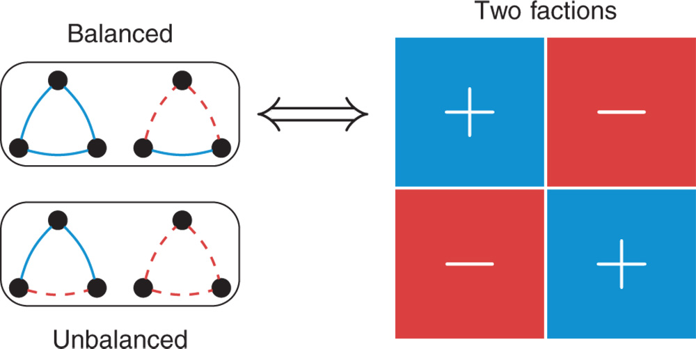
Figure 8.1 Structural balance. There are four possible configurations for having positive or negative links between three nodes (a triad). These are demonstrated on the left, where a solid line represents a positive link and a dashed line represents a negative link. The upper two triads are structurally balanced because the product of their signs is positive. Similarly, the lower two triads are not structurally balanced because the product of their signs is negative. If all triads (in a complete network) are structurally balanced, the network can be partitioned in two factions such that they are internally positively linked, with negative links between the two factions, as illustrated on the right.
For the remainder of the chapter, we restrict ourselves to undirected graphs. We first focus on complete graphs, where all links are present (excluding self-loops). Following [7], we provide the following definition.
Definition 8.1 A triad ![]() is called balanced whenever the product
is called balanced whenever the product
A complete signed graph ![]() is structurally balanced whenever all triads are balanced.
is structurally balanced whenever all triads are balanced.
Of the four possible triads, two are balanced (![]() and
and ![]() ) and two are unbalanced (
) and two are unbalanced (![]() and
and ![]() ) according to this definition (see also Figure 8.1).
) according to this definition (see also Figure 8.1).
Harary [18] proved that if the graph ![]() is structurally balanced, then it can be partitioned in two clusters such that there are only positive links within each cluster and negative links between them. Cartwright and Harary [7] called this observation the structure theorem, and Doreian and Mrvar [11] called it the first structure theorem.
is structurally balanced, then it can be partitioned in two clusters such that there are only positive links within each cluster and negative links between them. Cartwright and Harary [7] called this observation the structure theorem, and Doreian and Mrvar [11] called it the first structure theorem.
Theorem 8.1 (Structure theorem, [18]) Let ![]() be a complete signed graph. If and only if
be a complete signed graph. If and only if ![]() is balanced can
is balanced can ![]() be partitioned into two disjoint subsets
be partitioned into two disjoint subsets ![]() and
and ![]() such that a positive edge
such that a positive edge ![]() either in
either in ![]() or
or ![]() while a negative edge
while a negative edge ![]() falls in
falls in ![]() .
.
Proof: Assume ![]() is balanced. Consider some node
is balanced. Consider some node ![]() and set
and set ![]() as well as the set
as well as the set ![]() . Consider an edge
. Consider an edge ![]() . Then
. Then ![]() and
and ![]() by definition of
by definition of ![]() so that
so that ![]() by structural balance. Hence all edges in
by structural balance. Hence all edges in ![]() are positive. Similarly, any edge
are positive. Similarly, any edge ![]() is positive. Hence, we can partition
is positive. Hence, we can partition ![]() into the stated disjoint sets
into the stated disjoint sets ![]() and
and ![]() . In reverse, any triad is easily seen to be balanced if
. In reverse, any triad is easily seen to be balanced if ![]() is partitioned as stated in the theorem.
is partitioned as stated in the theorem.
While the above is limited to complete graphs, it can be generalized to incomplete graphs. For this we first need to introduce another definition for structural balance.
Definition 8.2 (Structural Balance) Let ![]() be a signed graph and
be a signed graph and ![]() the signed adjacency matrix. Let
the signed adjacency matrix. Let ![]() be a cycle consisting of nodes
be a cycle consisting of nodes ![]() with
with ![]() . Then the cycle
. Then the cycle ![]() is called balanced whenever
is called balanced whenever

A signed graph ![]() is called balanced if all its cycles
is called balanced if all its cycles ![]() are balanced.
are balanced.
Stated differently, ![]() is the sign of the cycle which is balanced if its sign is positive. If a cycle contains
is the sign of the cycle which is balanced if its sign is positive. If a cycle contains ![]() negative edges, then
negative edges, then ![]() . In other words, a cycle is balanced if it contains an even number of negative links. Note that for a cycle of length three, this coincides exactly with the definition of a balanced triad.
. In other words, a cycle is balanced if it contains an even number of negative links. Note that for a cycle of length three, this coincides exactly with the definition of a balanced triad.
The sign of a cycle can be decomposed in the sign of subcycles if the cycle has a chord: an edge between two nodes of the cycle (see Figure 8.2).
Theorem 8.2 Let ![]() be a cycle with a chord between nodes
be a cycle with a chord between nodes ![]() and
and ![]() in
in ![]() . Then let
. Then let ![]() and
and ![]() be the induced subcycles. Then
be the induced subcycles. Then ![]() .
.
Proof: We denote by ![]() the number of negative links of
the number of negative links of ![]() and similarly
and similarly ![]() for
for ![]() and
and ![]() for
for ![]() . Suppose that the link
. Suppose that the link ![]() is not a negative link. Then the number of negative links in
is not a negative link. Then the number of negative links in ![]() is
is ![]() so that
so that ![]() . Suppose that
. Suppose that ![]() is a negative link. Then
is a negative link. Then ![]() so that
so that ![]() .
.
In other words, it is not necessary to determine the structural balance of all cycles, and we can restrict ourselves to the balance of chordless cycles. In fact, this statement can be made stronger, and holds for any combination of cycles. With a combination of cycles, we mean the symmetric difference of the edges of the two cycles. To define this properly it is more convenient to denote a cycle by the set of its edges (in no particular order). That is, we define a cycle ![]() where the edges form a cycle, i.e. the subgraph of
where the edges form a cycle, i.e. the subgraph of ![]() is a cycle.
is a cycle.

Figure 8.2 Chords and cycles. This illustrates a cycle  with a chord between nodes
  and
and  . There are two subcycles: one following the left path and the other following the right path in the illustration. These two subcycles have a single common edge:
  . The sign of the large cycle is then the product of the sign of the two subcycles.
Definition 8.3 Let ![]() and
and ![]() be two cycles. Then we define the symmetric difference as
be two cycles. Then we define the symmetric difference as
We also refer to this as the combination of two cycles.
Note that the combination of two cycles may actually be a set of multiple edge-disjoint cycles.
Now we can prove the stronger statement on the combination of cycles.
Theorem 8.3 Let ![]() and
and ![]() be two cycles. If
be two cycles. If ![]() then
then ![]() .
.
Proof: Let us denote the number of negative links in a set ![]() by
by ![]() . Let
. Let ![]() be the union of the two cycles, and
be the union of the two cycles, and ![]() be the overlap of the two cycles. Then
be the overlap of the two cycles. Then ![]() , and
, and ![]() . Hence
. Hence
since ![]() for any integer
for any integer ![]() .
.
In other words, if we know the balance of some limited number of cycles, we can determine the balance of all cycles. These “limited number of cycles” are called the fundamental cycles. Any cycle can be obtained as a combination of two (or more) fundamental cycles. This implies that if all fundamental cycles are balanced, then the graph as a whole is balanced. We do not consider fundamental cycles in more detail, but this notion underlies the technique by Altafini [2] which we consider in Section 8.3.1.2.
Similar to the sign of cycles, we can define the sign of a path.
Definition 8.4 Let ![]() be a path in a signed graph
be a path in a signed graph ![]() with signed adjacency matrix
with signed adjacency matrix ![]() . The sign of the path
. The sign of the path ![]() is then defined as
is then defined as

Paths in signed networks are either positive or negative. A cycle can be decomposed in two paths so the sign of a cycle is the product of the sign of the two paths. Hence, a cycle is balanced if the two paths have the same sign.
As before, the graph ![]() can be partitioned in two clusters with positive links within clusters and negative links between clusters.
can be partitioned in two clusters with positive links within clusters and negative links between clusters.
Theorem 8.4 (Structure theorem, [18]) Let ![]() be a connected signed graph and
be a connected signed graph and ![]() the signed adjacency matrix. Then
the signed adjacency matrix. Then ![]() is balanced if and only if
is balanced if and only if ![]() can be partitioned into two disjoint subsets
can be partitioned into two disjoint subsets ![]() and
and ![]() such that a positive edge
such that a positive edge ![]() falls either in
falls either in ![]() or
or ![]() while a negative edge
while a negative edge ![]() falls in
falls in ![]() .
.
Proof First, assume ![]() is balanced. Then select any
is balanced. Then select any ![]() and set
and set ![]() , that is, all the nodes that can be reached through a positive path. Define
, that is, all the nodes that can be reached through a positive path. Define ![]() . Let
. Let ![]() . Suppose
. Suppose ![]() . By construction of
. By construction of ![]() , then both
, then both ![]() and
and ![]() have a positive path to
have a positive path to ![]() , so that the path
, so that the path ![]() through
through ![]() is also positive. But if
is also positive. But if ![]() is negative, it would be contained in a negative cycle, contradicting balance. Hence
is negative, it would be contained in a negative cycle, contradicting balance. Hence ![]() . Similarly, suppose that
. Similarly, suppose that ![]() . Then both the
. Then both the ![]() path and the
path and the ![]() path are negative (otherwise
path are negative (otherwise ![]() and
and ![]() would be in
would be in ![]() ). The
). The ![]() path through
path through ![]() is then positive since the product of the two negative paths is positive. Again, since
is then positive since the product of the two negative paths is positive. Again, since ![]() this contradicts balance. Hence, all negative edges lie between
this contradicts balance. Hence, all negative edges lie between ![]() and
and ![]() . Finally, let
. Finally, let ![]() with
with ![]() and
and ![]() . Then there is a positive
. Then there is a positive ![]() path and a negative
path and a negative ![]() path, so that the
path, so that the ![]() path through
path through ![]() is negative, which combined with the positive edge
is negative, which combined with the positive edge ![]() leads to a negative cycle, contradicting balance. Hence, positive edges lie within
leads to a negative cycle, contradicting balance. Hence, positive edges lie within ![]() and
and ![]() . We conclude that if
. We conclude that if ![]() is balanced, it can be partitioned as stated. Vice versa, suppose
is balanced, it can be partitioned as stated. Vice versa, suppose ![]() can be partitioned into the two states subsets
can be partitioned into the two states subsets ![]() and
and ![]() . Let
. Let ![]() be a cycle. If
be a cycle. If ![]() is contained within
is contained within ![]() or
or ![]() it is completely positive, so that
it is completely positive, so that ![]() . Suppose
. Suppose ![]() has some node
has some node ![]() and
and ![]() . Then any
. Then any ![]() path contains an odd number of negative links, and is hence negative, so that the cycle
path contains an odd number of negative links, and is hence negative, so that the cycle ![]() is positive. Hence, all cycles are balanced, and so
is positive. Hence, all cycles are balanced, and so ![]() is balanced.
is balanced.
8.2.1 Weak Structural Balance
Classical structural balance theory predicts that a balanced network can be partitioned into two clusters. However, as suggested by Davis [9] and Cartwright and Harary [8], we can generalize this notion of structural balance by redefining the notion of an unbalanced triad or cycle. Consider, for example, the (unbalanced) triad with three negative links. The three nodes can be partitioned into three clusters: trivially, all links between clusters are negative and all positive links are within clusters. There is a simple characterization of networks that can be partitioned in such a way: no cycle can contain exactly one negative link. Davis [9] established this only for complete graphs, and Cartwright and Harary [8] extended it to sparse graphs. We call signed networks with this property weakly structurally balanced (or weakly balanced).
Definition 8.5 A cycle ![]() is termed weakly balanced if it does not contain exactly a single negative link. A signed graph
is termed weakly balanced if it does not contain exactly a single negative link. A signed graph ![]() is called weakly balanced if all its cycles
is called weakly balanced if all its cycles ![]() are weakly balanced.
are weakly balanced.
Following this, we can call the previous definition strong structural balance. Any graph that is strongly structurally balanced is also weakly structurally balanced: a cycle with a positive sign must contain an even number of negative links. It cannot have exactly one. The reverse does not hold: a weakly structurally balanced cycle can have three negative links, which is not allowed in strong structural balance.
Lemma 8.0 Let ![]() be a cycle with a chord between nodes
be a cycle with a chord between nodes ![]() and
and ![]() in
in ![]() . Then let
. Then let ![]() and
and ![]() be the induced subcycles. Then
be the induced subcycles. Then ![]() is weakly balanced if
is weakly balanced if ![]() and
and ![]() are weakly balanced.
are weakly balanced.
Proof: We denote by ![]() the number of negative links of
the number of negative links of ![]() and, similarly,
and, similarly, ![]() for
for ![]() and
and ![]() for
for ![]() . Suppose that the link
. Suppose that the link ![]() is not a negative link, then the number of negative links in
is not a negative link, then the number of negative links in ![]() is
is ![]() , implying
, implying ![]() is weakly balanced. Suppose that
is weakly balanced. Suppose that ![]() is a negative link. Then both
is a negative link. Then both ![]() and
and ![]() , and
, and ![]() so that
so that ![]() is weakly balanced.
is weakly balanced.
The inverse does not hold. This can readily be seen by considering an all-positive cycle with a single negative chord. The all-positive cycle, clearly, is weakly balanced, but the induced sub-cycles contain exactly one single negative link, and are therefore not weakly balanced. The theorem on chordless cycles for weak balance is hence a weaker statement than the corresponding theorem for strong structural balance. Nonetheless, we can still limit ourselves to considering chordless cycles for determining whether a graph is weakly structurally balanced.
Theorem 8.6 Let ![]() be a signed network. Then
be a signed network. Then ![]() is weakly structurally balanced if and only if all chordless cycles are weakly structurally balanced.
is weakly structurally balanced if and only if all chordless cycles are weakly structurally balanced.
Proof: If ![]() is weakly balanced, all cycles are balanced, so that trivially all chordless cycles are balanced. Vice versa, assume all chordless cycles are weakly balanced. We use induction on
is weakly balanced, all cycles are balanced, so that trivially all chordless cycles are balanced. Vice versa, assume all chordless cycles are weakly balanced. We use induction on ![]() . All chordless cycles
. All chordless cycles ![]() are balanced by assumption, providing our inductive base for
are balanced by assumption, providing our inductive base for ![]() (because triads are chordless by definition). Assume all cycles with
(because triads are chordless by definition). Assume all cycles with ![]() are balanced, then consider cycle
are balanced, then consider cycle ![]() of length
of length ![]() . If
. If ![]() contains a chord, we can separate
contains a chord, we can separate ![]() in cycles
in cycles ![]() and
and ![]() , which are balanced by our inductive assumption. Then, by Lemma 8.5 cycle
, which are balanced by our inductive assumption. Then, by Lemma 8.5 cycle ![]() is balanced. Hence, all cycles are weakly balanced.
is balanced. Hence, all cycles are weakly balanced.
To determine whether a graph is weakly structurally balanced, we need only consider the chordless cycles rather than all cycles. Computationally, this is important.
Similar to strong structural balance, we can partition a weakly structurally balanced graph, but now in possibly more than two clusters. This is called the second structure theorem by Doreian and Mrvar [11].
Theorem 8.7 (Clusterability theorem, [8]) Let ![]() be a connected signed graph. Then
be a connected signed graph. Then ![]() is weakly structurally balanced if and only if
is weakly structurally balanced if and only if ![]() can be partitioned into disjoint subsets
can be partitioned into disjoint subsets ![]() such that a positive edge
such that a positive edge ![]() falls in
falls in ![]() while a negative edge
while a negative edge ![]() falls in
falls in ![]() for
for ![]() .
.
Proof: Suppose ![]() is weakly balanced. Let
is weakly balanced. Let ![]() be the positive part of the signed graph, and let the clusters be defined by the connected components of
be the positive part of the signed graph, and let the clusters be defined by the connected components of ![]() . Any positive edge then clearly cannot fall between clusters because different connected components cannot be connected through a positive link. Consider then some negative link
. Any positive edge then clearly cannot fall between clusters because different connected components cannot be connected through a positive link. Consider then some negative link ![]() . Suppose that
. Suppose that ![]() and
and ![]() are both in some
are both in some ![]() . Then there exists a positive
. Then there exists a positive ![]() path because they are in the same component, thus yielding a cycle with exactly a single negative link, contradicting weak balance. Hence, any negative link falls between clusters. Vice versa, suppose
path because they are in the same component, thus yielding a cycle with exactly a single negative link, contradicting weak balance. Hence, any negative link falls between clusters. Vice versa, suppose ![]() is split into clusters as stated in the theorem. Any cycle completely contained within a cluster has only positive links. Consider a cycle through
is split into clusters as stated in the theorem. Any cycle completely contained within a cluster has only positive links. Consider a cycle through ![]() and
and ![]() where
where ![]() and
and ![]() ,
, ![]() . Then any path between
. Then any path between ![]() and
and ![]() must contain at least a single negative link, so that any cycle must contain at least two negative links.
must contain at least a single negative link, so that any cycle must contain at least two negative links.
It is easy to see when a complete signed graph is weakly structurally balanced: it must not contain the ![]() triad.
triad.
In summary, signed networks which are strongly structurally balanced can be partitioned in two clusters. Signed networks which are weakly structurally balanced can be partitioned in multiple clusters. Clearly, all signed networks which are strongly structurally balanced are also weakly structurally balanced, but not vice versa. One obvious question is whether strong or weak structural balance is more realistic. This led to partitioning signed networks, which we examine in the next section.
8.3 Partitioning
The previous section introduced the general idea and structure theorems for structural balance. However, these conditions are rather strict: no cycle can exist with an odd number of negative links (strong balance) or a single negative link (weak balance). Empirically, this is rather unrealistic to achieve exactly, but we might come close. This was suggested by Cartwright and Harary [7], when introducing the notion of structural balance, who suggested counting the number of cycles that are balanced and measuring the proportion of balanced cycles, termed the degree of balance:

where ![]() is the number of balanced cycles and
is the number of balanced cycles and ![]() is the total number of cycles. This measure is used infrequently because it is computationally intensive to list all cycles [23]. The number of cycles in a graph increases exponentially with its size. Depending on the so-called cyclomatic number,
is the total number of cycles. This measure is used infrequently because it is computationally intensive to list all cycles [23]. The number of cycles in a graph increases exponentially with its size. Depending on the so-called cyclomatic number, ![]() , there are between
, there are between ![]() and
and ![]() cycles [36], which Harary [19] also uses to define bounds on the degree of balance. However, this number provides little insight into the structure of the network.
cycles [36], which Harary [19] also uses to define bounds on the degree of balance. However, this number provides little insight into the structure of the network.
A more useful measure was suggested by Harary [19]: the smallest number of ties to be deleted in order to make the network (weakly) balanced. This is the same as the number of ties whose reversal of signs leads to a balanced network. This is known as the line index of imbalance. Computing the line index of imbalance is computationally intensive as it is an NP-hard problem. Initially the definition was restricted to strong structural balance. Doreian and Mrvar [11] were the first to introduce this in the context of clustering for weak structural balance.
8.3.1 Strong Structural Balance
Given a partition into two subsets, ![]() and
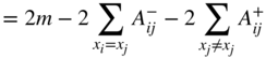
and ![]() , we can measure the number of edges that are in conflict with structural balance. The number of negative edges within
, we can measure the number of edges that are in conflict with structural balance. The number of negative edges within ![]() are
are

and similarly so for ![]() , while the positive edges between
, while the positive edges between ![]() and
and ![]() are
are

so that the total number of edges inconsistent with structural balance for a partition into ![]() and
and ![]() is
is
This is the line index of imbalance mentioned earlier. A graph ![]() is then structurally balanced if and only if the minimum line index of imbalance is zero.
is then structurally balanced if and only if the minimum line index of imbalance is zero.
8.3.1.1 Spectral Theory
Given a partition into ![]() and
and ![]() , let
, let ![]() if
if ![]() and
and ![]() if
if ![]() . Then for an edge
. Then for an edge ![]() , if
, if ![]() then
then ![]() , while for
, while for ![]() we have
we have ![]() . Hence
. Hence


So that ![]() gives (twice) the number of edges that are consistent with balance, the inverse of the line index of imbalance. Note that this also implies that if
gives (twice) the number of edges that are consistent with balance, the inverse of the line index of imbalance. Note that this also implies that if ![]() is the partition corresponding to structural balance, then
is the partition corresponding to structural balance, then ![]() for all
for all ![]() ,
, ![]() .
.
Theorem 8.8 Let ![]() be a connected signed graph and let
be a connected signed graph and let ![]() be the dominant eigenvector of the signed adjacency matrix
be the dominant eigenvector of the signed adjacency matrix ![]() . Then
. Then ![]() is balanced if and only if
is balanced if and only if ![]() and
and ![]() defines the split into two clusters as in Theorem 8.4.
defines the split into two clusters as in Theorem 8.4.
Proof: If the split defines a correct partition, then obviously ![]() is balanced (Theorem 8.4). In reverse, suppose
is balanced (Theorem 8.4). In reverse, suppose ![]() is balanced. Let
is balanced. Let ![]() be the dominant eigenvector. Suppose that
be the dominant eigenvector. Suppose that ![]() for some
for some ![]() . Then let
. Then let ![]() be another vector with
be another vector with ![]() for all
for all ![]() and
and ![]() for all
for all ![]() , which is possible by structural balance of
, which is possible by structural balance of ![]() . Then
. Then ![]() and
and


which contradicts the fact that ![]() is the dominant eigenvector. Hence,
is the dominant eigenvector. Hence, ![]() for all
for all ![]() and it defines a correct partition.
and it defines a correct partition.
The vector space constrained to ![]() is rather difficult to optimize. Taking general vectors with
is rather difficult to optimize. Taking general vectors with ![]() , the dominant eigenvector
, the dominant eigenvector ![]() maximizes this and the largest eigenvalue of the adjacency matrix
maximizes this and the largest eigenvalue of the adjacency matrix ![]() gives a lower bound of the line index of imbalance.
gives a lower bound of the line index of imbalance.
Kunegis et al. [26] suggest using the signed Laplacian [21] for measuring structural balance. It is defined as
where ![]() is the signed adjacency matrix as defined earlier and
is the signed adjacency matrix as defined earlier and ![]() the diagonal matrix of total degrees. The rows of
the diagonal matrix of total degrees. The rows of ![]() sum to twice the negative degrees
sum to twice the negative degrees ![]() because
because ![]() , so that
, so that ![]() . Furthermore, the Laplacian is positive-semidefinite, i.e.
. Furthermore, the Laplacian is positive-semidefinite, i.e. ![]() for all
for all ![]() . We can show this as follows. Writing this out, we obtain
. We can show this as follows. Writing this out, we obtain

Since ![]() , we can write
, we can write ![]() and obtain
and obtain

Clearly ![]() so that we get
so that we get

which can be nicely expressed as a square (because ![]() and
and ![]() )
)

Now suppose ![]() is strongly balanced so that we can partition the nodes into
is strongly balanced so that we can partition the nodes into ![]() and
and ![]() without violating balance. Let
without violating balance. Let ![]() if
if ![]() and
and ![]() if
if ![]() . Then for any edge
. Then for any edge ![]() , if
, if ![]() then by strong balance
then by strong balance ![]() , while if
, while if ![]() we have
we have ![]() . Hence
. Hence ![]() and the smallest eigenvalue of the Laplacian is 0. Vice versa, if the Laplacian is 0,
and the smallest eigenvalue of the Laplacian is 0. Vice versa, if the Laplacian is 0, ![]() is balanced: the term
is balanced: the term ![]() can only be 0 for all
can only be 0 for all ![]() if
if ![]() is balanced.
is balanced.
More generally, given a partition into ![]() and
and ![]() , let
, let ![]() if
if ![]() and
and ![]() if
if ![]() . Then for an edge
. Then for an edge ![]() , if
, if ![]() then
then ![]() while if
while if ![]() then
then ![]() . Hence,
. Hence,


and the vector ![]() gives (twice) the line index of imbalance.
gives (twice) the line index of imbalance.
The vector space constrained to ![]() is rather difficult to optimize. Taking general vectors with
is rather difficult to optimize. Taking general vectors with ![]() , the minimal eigenvector
, the minimal eigenvector ![]() minimizes
minimizes ![]() . Consequentially, the smallest eigenvalue of the Laplacian
. Consequentially, the smallest eigenvalue of the Laplacian ![]() gives a lower bound of the line index of imbalance, as
gives a lower bound of the line index of imbalance, as ![]() where
where ![]() is the smallest eigenvector. The partition induced by
is the smallest eigenvector. The partition induced by ![]() , however, taking
, however, taking ![]() , i.e.
, i.e. ![]() , gives an upper bound, as the minimum index of imbalance is at most the index of an actual partition. Hence, we obtain
, gives an upper bound, as the minimum index of imbalance is at most the index of an actual partition. Hence, we obtain
where ![]() .
.
We thus obtain the identity that ![]() and that maximizing
and that maximizing ![]() is equivalent to minimizing
is equivalent to minimizing ![]() . However, the eigenvectors of the adjacency matrix and the Laplacian are, in general, not identical. In the case of balanced graphs though, the largest eigenvector of the adjacency matrix and the smallest eigenvector of the Laplacian provide identical information: the partition into
. However, the eigenvectors of the adjacency matrix and the Laplacian are, in general, not identical. In the case of balanced graphs though, the largest eigenvector of the adjacency matrix and the smallest eigenvector of the Laplacian provide identical information: the partition into ![]() and
and ![]() .
.
8.3.1.2 Switching
One interesting observation in signed graph theory is that we can change the sign of some links without affecting balance. More precisely, we can switch the signs of edges across a cut without changing structural balance. Switching signs was introduced originally by Abelson and Rosenberg [1], who used it to calculate the line index of imbalance (although they called it the “complexity” of a signed graph). This was later used by Zaslavsky [37] in a formal graph-theoretical setting. More recently, Iacono et al. [24] use sign switches in an algorithm for calculating the line index of imbalance.
Definition 8.6 (Switching) Let ![]() be a signed graph with signed adjacency matrix
be a signed graph with signed adjacency matrix ![]() and let
and let ![]() and
and ![]() be a partition of
be a partition of ![]() . Then let
. Then let ![]() if
if ![]() and
and ![]() if
if ![]() , with
, with ![]() and define
and define ![]() so that
so that ![]() . Then the graph
. Then the graph ![]() defined by
defined by ![]() is called a switching of
is called a switching of ![]() defined by the partition
defined by the partition ![]() and
and ![]() .
.
Hence, for a link ![]() with
with ![]() and
and ![]() , then
, then ![]() , while if both
, while if both ![]() (or
(or ![]() ),
), ![]() . In other words, switching means we invert the signs of links across the cut by the partition
. In other words, switching means we invert the signs of links across the cut by the partition ![]() and
and ![]() , as illustrated in Figure 8.3. Most importantly, any switching preserves the balance of any cycle.
, as illustrated in Figure 8.3. Most importantly, any switching preserves the balance of any cycle.

Figure 8.3 Switching. On the left, there are three edges crossing the partition into  and
and  : two negative (the dashed lines) and one positive (the solid line). When we switch according to the partition
  and
and  , this implies that we switch the signs of the edges crossing the partition, but leave all the other signs unchanged. This is illustrated on the right. All cycles keep the same sign after the switching. In this case this reduces the number of negative links and simplifies finding the balanced partition. The balanced partition is indicated by black and white nodes in both cases. On the right, the black and white are reversed for
  , corresponding to the switching of the balanced partition by
  and
and  as explained in Theorem 8.10.
Theorem 8.9 Let ![]() be a signed graph and let
be a signed graph and let ![]() be a switched signed graph. Denote by
be a switched signed graph. Denote by ![]() the sign of some cycle
the sign of some cycle ![]() with respect to
with respect to ![]() . Then for any cycle
. Then for any cycle ![]() ,
, ![]() .
.
Proof: Let ![]() be a cycle and let
be a cycle and let ![]() and
and ![]() be a partition of
be a partition of ![]() . Let
. Let ![]() be the number of positive/negative links across the cut between
be the number of positive/negative links across the cut between ![]() and
and ![]() in
in ![]() and
and ![]() the number of positive/negative links within
the number of positive/negative links within ![]() or
or ![]() . Then
. Then ![]() . Hence there are
. Hence there are ![]() and
and ![]() across the cut in
across the cut in ![]() , while
, while ![]() . By definition
. By definition ![]() is even since any cycle must cross
is even since any cycle must cross ![]() and
and ![]() an even number of times. In other words,
an even number of times. In other words, ![]() and hence
and hence ![]() . We thus obtain
. We thus obtain
Recall that the line index of imbalance is the minimum number of signs that would need to be changed to make the graph structurally balanced. So, if the balance of the cycles does not change, then neither would the minimum number of sign changes required, and hence the line index of imbalance remains the same.
Theorem 8.10 Let ![]() {−1,1} be a partition of
{−1,1} be a partition of ![]() and let
and let ![]() be a switching of
be a switching of ![]() . Then the switched partition
. Then the switched partition ![]() has the same imbalance for the switched graph
has the same imbalance for the switched graph ![]() .
.
Proof: The imbalance the partition ![]() on
on ![]() is
is ![]() , and for the switched partition and graph we have
, and for the switched partition and graph we have
because ![]() .
.
Even if the partition itself is not balanced, switching is defined for any partition. If ![]() is balanced, we can take the balanced partition
is balanced, we can take the balanced partition ![]() and
and ![]() , in which case all the negative links become positive (because they fall between
, in which case all the negative links become positive (because they fall between ![]() and
and ![]() ), so that we end up with a completely positive graph. In reverse, the same thing holds: if we can find a switching
), so that we end up with a completely positive graph. In reverse, the same thing holds: if we can find a switching ![]() such that
such that ![]() is completely positive,
is completely positive, ![]() is balanced, and the switching
is balanced, and the switching ![]() defines the optimal partition (see also Hou et al. [21]). The same principle does not hold for weak structural balance. For example, a triad with three negative links contains a single one after switching so that the original was weakly balanced but the switched one is not.
defines the optimal partition (see also Hou et al. [21]). The same principle does not hold for weak structural balance. For example, a triad with three negative links contains a single one after switching so that the original was weakly balanced but the switched one is not.
When Abelson and Rosenberg [1] introduced the idea of switching, they considered a node with the maximal difference of the positive and negative degree: ![]() . Switching the signs of all its links would then decrease the total number of negative links, while the balance would remain unchanged. The final number of negative links then gives an upper bound on the number of negative links that would need to be removed (or switched) in order to yield structural balance. In other words, it provides an upper bound on the line index of imbalance.
. Switching the signs of all its links would then decrease the total number of negative links, while the balance would remain unchanged. The final number of negative links then gives an upper bound on the number of negative links that would need to be removed (or switched) in order to yield structural balance. In other words, it provides an upper bound on the line index of imbalance.
More recently, a rather similar approach was used by Iacono et al. [24]. They follow the same procedure as Abelson and Rosenberg [1] for reducing the number of negative links to arrive at an upper bound for the line index of imbalance. The optimal solution may contain even fewer negative links. Iacono et al. [24] also provide a way to arrive at a lower bound. The key idea is to associate each negative link to an edge-independent unbalanced cycle, which is easier if the graph contains few negative links. This procedure relies on the fundamental cycles we briefly encountered earlier. Clearly at least one link must change for each edge-independent unbalanced cycle. Even though some cut set may reduce the number of negative links, no cut set can reduce it more than the number of unbalanced edge-independent cycles. Hence, this provides a lower bound on the line index of imbalance.
8.3.2 Weak Structural Balance
The previous subsection dealt only with a split in two factions. We can provide similar definitions for a split in multiple factions. In particular, the number of inconsistencies with structural balance for a given partition into ![]() is
is

Note that if a network contains only positive or only negative links, the minimum line index of imbalance is, by definition, 0. For a network of only positive links, the trivial partition consisting of a single cluster provides such a solution. Similarly, for a network of only negative links, the trivial partition consisting of each node in its own cluster, commonly called the singleton partition, achieves zero imbalance.
However, if all links are negative there is an interesting problem: finding the minimum number of factions required for obtaining an imbalance of 0. Having ![]() factions (clusters), with each node in its own faction with an imbalance measure of 0, most often, has little value. It is reasonable to think that this measure could be achieved with fewer factions. For example, for a bipartite graph with all negative links, we have to use only two factions. This minimum number of factions necessary to obtain an imbalance of 0 is known also as the chromatic number: the minimum number of colors necessary to color each node such that two nodes that are connected have different colors. This is a much studied area of research in graph theory. It is an NP-complete problem. This connection was recognized by Cartwright and Harary [8]. The similar problem for positive links is oddly enough trivial: the maximum number of communities for which the imbalance is still 0 simply corresponds to the connected components.
factions (clusters), with each node in its own faction with an imbalance measure of 0, most often, has little value. It is reasonable to think that this measure could be achieved with fewer factions. For example, for a bipartite graph with all negative links, we have to use only two factions. This minimum number of factions necessary to obtain an imbalance of 0 is known also as the chromatic number: the minimum number of colors necessary to color each node such that two nodes that are connected have different colors. This is a much studied area of research in graph theory. It is an NP-complete problem. This connection was recognized by Cartwright and Harary [8]. The similar problem for positive links is oddly enough trivial: the maximum number of communities for which the imbalance is still 0 simply corresponds to the connected components.
8.3.3 Blockmodeling
The original blockmodel function proposed by Doreian and Mrvar [11] is exactly equivalent to the line index of imbalance. They also propose a more general form, however, weighting differently positive or negative violations of balance:
where ![]() returns (half) the original line index. However, this generality comes with costs. Without surprise, different values for
returns (half) the original line index. However, this generality comes with costs. Without surprise, different values for ![]() return different values of
return different values of ![]() . More consequentially, different partitions of the nodes can be returned. This implies there is no principled way for selecting a value of
. More consequentially, different partitions of the nodes can be returned. This implies there is no principled way for selecting a value of ![]() and hence a partition. This issue was noted by Doreian and Mrvar [13]. It can be called “the alpha problem” which amounts to understanding the interplay of the number of positive and negative links in a signed network, the shape of the criterion function, and the role of
and hence a partition. This issue was noted by Doreian and Mrvar [13]. It can be called “the alpha problem” which amounts to understanding the interplay of the number of positive and negative links in a signed network, the shape of the criterion function, and the role of ![]() in determining partitions.
in determining partitions.
The blockmodeling approach partitions the nodes into positions and the links into blocks, which are the sets of links between nodes in the positions. There is only one type of blockmodel in accordance with structural balance: positive blocks on the main diagonal and negative blocks off the diagonal. Of course, for most empirical situations, the links contributing to the line index for imbalance are distributed across blocks. To address this, Doreian and Mrvar [12] examined other possible blockmodels. They considered two mutually antagonistic camps being mediated by a third group (either internally negative or not). So, rather than seeking a blockmodel consisting of diagonal positive blocks and off-diagonal negative blocks, they proposed blockmodels with positive and negative blocks appearing anywhere. For the empirical networks they studied, the results were better fits to the data, according to the line index, and more useful partitions. Unfortunately this comes at a price: if the number of clusters is left unspecified a priori, the best partition is the singleton partition (i.e. each node in its own cluster). This line of research is further studied in [5,15].
Stochastic block models can also deal with negative links [25], but we do not discuss them further here.
8.3.4 Community Detection
Assuming structural balance holds for a network, the resulting partition is a set of clusters with primarily positive ties within them. Structural balance models would not be informative for networks without negative ties. Even so, the positively connected clusters may contain some further substructure. Most networks that contain only positive links can show a clear group structure, commonly called the community structure or modular structure, covered in Chapter 4. One of the most popular methods for community detection in networks with only positive links is known as modularity. It is defined as

where it is assumed that ![]() only contains positive entries and
only contains positive entries and ![]() denotes the community of node
denotes the community of node ![]() (i.e. if
(i.e. if ![]() it means that node
it means that node ![]() is in community
is in community ![]() ) and where
) and where ![]() if
if ![]() and otherwise
and otherwise ![]() . Although this method suffers from a number of problems, most prominently the resolution limit [16], it seems to return sensible partitions for graphs with only positive links.
. Although this method suffers from a number of problems, most prominently the resolution limit [16], it seems to return sensible partitions for graphs with only positive links.
However, modularity suffers from a problem when some of the links are negative [17, 32]. In particular, imagine there are two fully connected subgraphs, the first with ![]() nodes and the second with only
nodes and the second with only ![]() nodes while there are
nodes while there are ![]() negative links between these two subgraphs. Using the ordinary definitions, the weighted degree for the first subgraph would be
negative links between these two subgraphs. Using the ordinary definitions, the weighted degree for the first subgraph would be ![]() because each node has four links to the other in the subgraph, and two negative links to the other subgraph. Similarly, the weighted degree for the second subgraph is
because each node has four links to the other in the subgraph, and two negative links to the other subgraph. Similarly, the weighted degree for the second subgraph is ![]() and the total weight is
and the total weight is ![]() . Hence, for any link within the first subgraph,
. Hence, for any link within the first subgraph,

and for the second subgraph
and for any link in between

This is rather surprising, as it says that two nodes that are positively connected should be split apart (their contribution is negative), while two negatively connected nodes should be kept together (their contribution is positive). Of course the correct partition here should be a partition into two communities: all nodes of the first subgraph form one community and all nodes of the second subgraph form the other. However, summing up the contributions in Equations 8.40 and 8.41 the quality of such a partition would be
while if there is only one single large partition, adding the contribution from Equation 8.42, we obtain
In short, modularity cannot be simply applied to signed networks, as the results are inconsistent with the correct partition (cf. [13]). Hence, modularity needs to be corrected in some way to account for the presence of negative links for it to be useful for signed networks.
Consistent with structural balance, we would expect negative links to be between communities, while positive links are within communities. Hence, if we define the quality of the partition on the positive part as

and on the negative part as

then we should like to maximize ![]() and minimize
and minimize ![]() . We can do this by combining
. We can do this by combining ![]() , which then becomes
, which then becomes

where ![]() as throughout this chapter. In essence, this comes down to using a null model that is adapted to signed networks. More details can be found in Traag [31, Chapter 5].
as throughout this chapter. In essence, this comes down to using a null model that is adapted to signed networks. More details can be found in Traag [31, Chapter 5].
More generally speaking, one could always define ![]() for a partition on the positive subnetwork and
for a partition on the positive subnetwork and ![]() on the negative subnetwork and then define a new quality function as
on the negative subnetwork and then define a new quality function as ![]() . For some methods this turns out to give quite nice results, for example for the Constant Potts Model (CPM) [33]. This method was introduced to circumvent any particular form of the resolution limit. The formulation (again assuming
. For some methods this turns out to give quite nice results, for example for the Constant Potts Model (CPM) [33]. This method was introduced to circumvent any particular form of the resolution limit. The formulation (again assuming ![]() is only positive) is simple:
is only positive) is simple:

Here ![]() plays the role of a resolution parameter, which needs to be chosen in some way. This parameter has a nice interpretation though, which could motivate a particular parameter setting, and functions as a sort of threshold. In any optimal partition, the density between any two communities is no higher than
plays the role of a resolution parameter, which needs to be chosen in some way. This parameter has a nice interpretation though, which could motivate a particular parameter setting, and functions as a sort of threshold. In any optimal partition, the density between any two communities is no higher than ![]() . Put differently,
. Put differently, ![]() , where
, where ![]() is the number of edges between
is the number of edges between ![]() and
and ![]() , and
, and ![]() and
and ![]() are the number of nodes in that community. Similarly, any community has a density of at least
are the number of nodes in that community. Similarly, any community has a density of at least ![]() , i.e.
, i.e. ![]() . Even stronger, in fact, any subset of a community is connected to the rest of its community with a density of at least
. Even stronger, in fact, any subset of a community is connected to the rest of its community with a density of at least ![]() in an optimal partition.
in an optimal partition.
If we extend our previous suggestion of combining the positive and negative parts we arrive at the following:

which, by setting ![]() , leads to
, leads to
In other words, for CPM, there is no need to treat negative links separately and we can immediately apply the same method.
Finally, for ![]() , CPM is equivalent to optimizing the line index of imbalance. Indeed, note that we can write the line index of imbalance as
, CPM is equivalent to optimizing the line index of imbalance. Indeed, note that we can write the line index of imbalance as

We can rewrite this as

so that ![]() for the CPM definition of
for the CPM definition of ![]() .
.
Given any particular quality function, the problem is always how to find a particular partition that maximizes this quality function. In general, this problem cannot be solved efficiently (it is NP-hard) and so we have to employ heuristics. One of the best performing algorithms for optimizing modularity is the so-called Louvain algorithm [3]. It can be adapted for taking into account negative links. In addition, it can also be adapted for CPM (and other quality functions). See https://pypi.python.org/pypi/louvain/ for a Python implementation designed for handling negative links and working with these various methods.
We do not discuss in detail how the algorithm works, but do discuss one particular element that needs to be changed for dealing with negative links. The basic ingredient of the algorithm is that it moves nodes to the best possible community. Ordinarily, in community detection, all communities are connected, and hence the algorithm only needs to consider moving nodes to neighboring communities. However, this property no longer holds when negative links are present. A trivial example is a fully connected bipartite graph with all negative links. In that case, none of the nodes in any community are connected at all. When only considering neighboring communities, the algorithm never considers moving a node to a community to which it is not connected. In the end, if the algorithm starts from a singleton partition (i.e. each node in its own community), it will remain there. So, we need to calculate the change in ![]() for all communities, even if it is not connected to that community. Unfortunately this increases the computational time required for running the algorithm. Nonetheless, the algorithm is quite fast. Of course, it only provides a lower bound on the optimal quality value. Hence, for minimizing the line index of imbalance it only provides an upper bound.
for all communities, even if it is not connected to that community. Unfortunately this increases the computational time required for running the algorithm. Nonetheless, the algorithm is quite fast. Of course, it only provides a lower bound on the optimal quality value. Hence, for minimizing the line index of imbalance it only provides an upper bound.
8.3.4.1 Temporal Community Detection
One concern when studying the evolution of balance is that we also would like to track the partition over time. For example, if we have two network snapshots and we try to detect the partition minimizing the imbalance, there is an arbitrary assignment to the clusters ![]() and 1 (or 0 and 1) in the sense that simply relabeling the partition by exchanging the
and 1 (or 0 and 1) in the sense that simply relabeling the partition by exchanging the ![]() and 1 yields exactly the same imbalance. For two communities this is still reasonably limited, but for more communities the problem may become more difficult, especially when dealing with many snapshots throughout time.
and 1 yields exactly the same imbalance. For two communities this is still reasonably limited, but for more communities the problem may become more difficult, especially when dealing with many snapshots throughout time.
We rely on a method introduced by Mucha et al. [29] to do temporal community detection, while still accounting for negative links. Because this is not the core issue in this chapter, we discuss it only briefly. The idea is to create one large network, which contains all the snapshots of the same network. Then, each node represents a temporal node: a combination of a time snapshot and the original node. Without any links between the different snapshots, the large network would thus consist of as many connected components as there are snapshots (assuming each snapshot is connected). Each snapshot is commonly called a slice, and each link within a slice is called an intraslice link. We introduce additional interslice links, which connects two identical nodes in two consecutive time slices (i.e. they represent the same underlying node, but at a different time) with a certain strength, called the interslice coupling strength. This requires also some additional changes on the Louvain algorithm.
8.4 Empirical Analysis
Empirical research has shown that while few empirical networks are close to balance, at least they are much closer than can be expected at random. Hence, there is considerable evidence that structural balance holds to some extent, at least for weak balance. The evidence for strong structural balance is far more modest, with many exceptions present in the literature. In particular, the all negative triad was found relatively frequently by Szell et al. [30] contradicting strong structural balance. They found triads having a single negative link (which is the only triad that is weakly unbalanced) much more rarely. Overall, their evidence favors weak structural balance over strong structural balance. Contrary to dynamical models of sign change, they find that links almost never change sign. However, there is relatively little research into the dynamics of structural balance. Examples where this has been done include Hummon and Doreian [22], Doreian and Krackhardt [10], Marvel et al. [28], and Traag et al. [34].
We here briefly investigate the dynamics of the network of international relations, where structural balance is argued to play a role by Doreian and Mrvar [13]. We gathered data from the Correlates of War1 (CoW) dataset, which collects a variety of information about international relations. We create a signed network based on their latest data on alliances (v4.1), representing the positive links, and the militarized interstate disputes (MID, v4.1), representing the negative links. To arrive at a single weight for each link, we sum the different weights on alliances and MIDs for each dyad (a dyad can be involved in multiple alliances and multiple MIDs at the same time). Each MID generates an undirected (negative) link for all states that are involved on different sides. For example, if the USA and the UK were in conflict with Egypt and the USSR, then this would generate four negative links: US–Egypt, UK–Egypt, US–USSR and UK–USSR. The MID weight is set to ![]() so that the weight is in
so that the weight is in ![]() (see CoW documentation for more details). Each alliance generates a link for all dyads involved in the alliance. The weighting is more complicated, since no a priori weights are assigned. We chose to weigh a defense pact with a weight of
(see CoW documentation for more details). Each alliance generates a link for all dyads involved in the alliance. The weighting is more complicated, since no a priori weights are assigned. We chose to weigh a defense pact with a weight of ![]() , non-aggression by a weight of
, non-aggression by a weight of ![]() , and both neutrality and an entente by a weight of
, and both neutrality and an entente by a weight of ![]() . The single weight is then the sum of the alliance weight minus the sum of the MID weight. Note that a dyad may be involved in multiple MIDs and/or multiple alliances at the same time, so that the individual weight of a link is not necessarily restricted to
. The single weight is then the sum of the alliance weight minus the sum of the MID weight. Note that a dyad may be involved in multiple MIDs and/or multiple alliances at the same time, so that the individual weight of a link is not necessarily restricted to ![]() .
.
We find that structural balance does not follow any singular trend, and certainly does not converge to structural balance, and remains stable. The same was found by Doreian and Mrvar [13] and Vinogradova and Galam [35], where an earlier version of the CoW data was used. We detect communities using CPM with ![]() and use the approach by Iacono et al. [24], which we abbreviate as IRSA (after the authors). We ran the Louvain algorithm for CPM both with an unlimited number of communities (corresponding to weak structural balance) and also with the number of communities restricted to two (corresponding to strong structural balance).
and use the approach by Iacono et al. [24], which we abbreviate as IRSA (after the authors). We ran the Louvain algorithm for CPM both with an unlimited number of communities (corresponding to weak structural balance) and also with the number of communities restricted to two (corresponding to strong structural balance).
IRSA provides less stable results compared to the CPM estimates (see Figure 8.4). Perhaps with more computation time, more accurate results could be achieved. Even so, regardless of the method, no clear stability emerges. There are some large peaks of imbalance around World War II (WWII), which we discuss. But during the Cold War, and even after the Cold War, no particular convergence towards 0 imbalance is observed. This is not unreasonable, as the international system is subject to new shocks when new conflicts, some of which are major conflicts, emerge. Rather than settling at some level of balance, some unbalance remains in the system which never completely dissipates. Most often, the difference between strong and weak structural balance usually is not so large. This implies that a partition of nations into just two factions already explains much of the structure in international relations. At face value, this suggests that strong balance is at least a reasonable first approximation, and provides some evidence that strong balance is operating in the international system. It is likely that weak balance operates also, perhaps at different timescales. Nonetheless, there are some clear deviations in the patterns of imbalance.
In particular, both IRSA and CPM find that 1944 shows a large peak with an imbalance of 43.9 (CPM) or 47.4 (IRSA), whereas weak structural balance only has an imbalance of 3.14. For this time point, using weak balance may be more useful. This result is due to the large number of conflicts among various parties, which weak balance can accommodate, but which presents problems for strong balance (see Figure 8.5). Indeed, of the 1785 triads in this network, there are 411 strongly unbalanced triads, of which 406 are all-negative triads. The all-negative triad is considered unbalanced under strong balance, but balanced under weak balance. This leaves only five unbalanced triads under weak balance (although this does not preclude the existence of longer unbalanced cycles).

Figure 8.4 Balance timeline. The line index of imbalance using two different methods. The approach by Iacono et al. [24] only works for strong balance. The CPM approach can be applied to both the strong and weak balance. CPM seems to provide more stable results than the approach by Iacono et al. [24].
Many of the all-negative triads are attributable to conflict among nine different countries who were all in conflict with each other: France, Germany, Italy, Hungary, Bulgaria, Romania, Russia, Finland, and New Zealand. Many other countries were opposed to at least two others of this large conflict: Japan, for example, was in conflict with both Russia and New Zealand. These conflicts may be unrelated, but they serve to create an additional unbalanced triad (in the strong sense). The weakly unbalanced triads involve the UK and Turkey. The UK was allied with Portugal and Turkey, but Portugal was also allied with Spain (through the alliance between the dictators controlling both countries), which was in conflict with the UK. Turkey was allied with Germany, Hungary, and Iraq in addition to the UK while the UK was in conflict with both Germany and Hungary. At the same time, Germany was also in conflict with Hungary and Iraq, complicating things further. Clearly, WWII featured many dyadic conflicts, each with their own dynamics.
There is another interesting observation: weak structural balance is higher than strong structural balance for 1939. This should not be the case ordinarily, as the minimal imbalance in weak structural balance should always be lower than strong structural balance. This then seems due to the shift of alliances during WWII. Since the clustering also favors a certain continuity over time, it may be better to cluster countries in a more stable way, without accounting for short-term deviations. This is what seems to happen in 1939 (see Figure 8.6). In particular, Russia is still allied with Germany and Italy, while Russia is in conflict with the UK, France, and Belgium at that time. Similarly, Hungary is allied with Turkey, and Spain with Portugal. Surprisingly, the UK also had some conflict with the USA at that time according to the CoW data.
Finally, in more recent times the weak balance clustering seems increasingly unrealistic. This is due to the fact that even if some countries are only weakly positively connected, they are immediately considered as a single cluster. In 2010, for example, most of the world is grouped together in a single cluster, except Africa and some exceptions. Nonetheless, some clearly separate clusters exist. We therefore also detected clusters using CPM with ![]() for 2010. The results are shown in Figure 8.8. There are clearly different clusters in Africa, something missed completely when partitioning with weak structural balance. Africa is divided into a Central African bloc, a Western African bloc, and a Northern African bloc clustered with Arab nations in the Middle East, with the remainder of Africa scattered across other communities. The former USSR remains a separate community. The so-called West breaks into two communities: North and South America constitute a community whereas Europe becomes a separate community.
for 2010. The results are shown in Figure 8.8. There are clearly different clusters in Africa, something missed completely when partitioning with weak structural balance. Africa is divided into a Central African bloc, a Western African bloc, and a Northern African bloc clustered with Arab nations in the Middle East, with the remainder of Africa scattered across other communities. The former USSR remains a separate community. The so-called West breaks into two communities: North and South America constitute a community whereas Europe becomes a separate community.
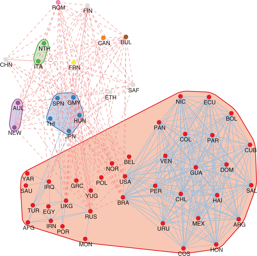
Figure 8.5 International relations 1944. The solid lines represent positive links and the dashed lines represent negative links. The countries that are clustered together are encircled.
At the height of the Cold War, we see the familiar division (see Figure 8.7). We also see the non-aligned states clustered outside of the familiar division. Yet some countries are clustered differently than what one would expect. For example, much of the Arab world is clustered with the West because of the alliance of Morocco and Libya with France, but note that Algeria is not as it was fighting a war of independence with France. Also, Yugoslavia is commonly seen as non-aligned in the Cold War, but here it is clustered with the West through its alliances with Greece and Turkey.

Figure 8.6 International relations 1939. The solid lines represent positive links and the dashed lines represent negative links. The countries that are clustered together are encircled.
This is also interesting from another perspective. Structural balance emphasizes both that negative links ought not exist within clusters and positive links ought not exist between clusters. This seems too restrictive by ignoring the presence of some conflict within clusters along with positive ties between clusters. Arguably, it makes more sense to allow for a few positive links between clusters without requiring them to be considered immediately a single cluster. Indeed, when using CPM with ![]() relatively less conflict happens within clusters, and most conflict takes place between clusters. Nonetheless, strong balance remains a reasonable first approximation.
relatively less conflict happens within clusters, and most conflict takes place between clusters. Nonetheless, strong balance remains a reasonable first approximation.
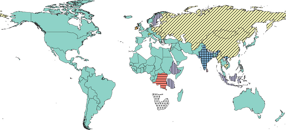
Figure 8.7 A map of the weak balance partition in 1962.
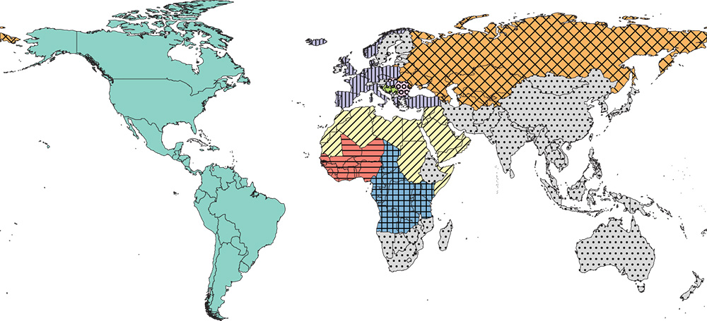
Figure 8.8 Map of CPM partition with  in 2010.
8.5 Summary and Future Work
Partitioning signed networks raises methodological issues that differ from those involved in partitioning unsigned networks. Various approaches have been developed. We started our discussion with a consideration of structural balance as it provides a substantively driven framework for considering signed networks. Formulated in terms of exact balance, the initial results in the literature take the form of existence theorems, which we discussed in some detail. We distinguished strong structural balance and weak structural balance. Empirically, most signed networks are not exactly balanced. One of the underlying assumptions of classical structural balance theory is that signed networks tends towards balance. To assess such a claim, it is necessary to have a measure of the extent to which a network is balanced or imbalanced. We discussed some of the measures in the literature but focused primarily on the line index of imbalance. Obtaining this measure is an NP-hard problem. We provided theorems regarding obtaining this measure and its upper and lower bounds.
In discussing strong structural balance, we considered spectral theory and presented some results showing how this is another useful approach for obtaining measures of imbalance. In doing so, we revisited the concept of switching. For partitioning signed networks, we considered signed blockmodeling as a method, pointing out its value and serious limitations. We considered community detection and outlined ways in which is can be adapted usefully to partition signed networks. In discussing this we considered also the Constant Potts Model and how it can be used to partition signed networks. We discussed briefly the notion of temporal community detection.
With the formal results in place, we turned to an empirical example using data from the Correlates of War (CoW) data. We applied two methods to obtain partitions for different points in time. We made no attempt to assess which is the “best” partitioning method, for they all have strengths and weaknesses. However, we did initiate a discussion regarding the conditions under which one method may perform better than others, without being universally the “best” under all conditions. This included a discussion of the utility of weak balance and strong balance, the number of clusters, and the temporal dynamics of the empirical network we studied.
Our results, consistent with other results for the CoW networks produced by others, is that, temporally, signed networks can move towards balance at some time points and away from balance at others. The assumption that signed networks tend towards balance had unfortunate consequences. The more important question, substantively, is simple to state: What are the conditions under which these changes take place? To some extent, this mirrors the issue of when some methods work better than others. The two are related. Together, these issues will form a focus for our future work both analytically and substantively.
References
- 1. R. P. Abelson and M. J. Rosenberg. Symbolic psycho-logic: A model of attitudinal cognition. Behavioral Science, 3(1):1–13, 1958.
- 2. C. Altafini. Dynamics of opinion forming in structurally balanced social networks. PLoS One, 7(6):e38135, 2012.
- 3. V. D. Blondel, J.-L. Guillaume, R. Lambiotte, and E. Lefebvre. Fast unfolding of communities in large networks. Journal of Statistical Mechanics, 10008(10):6, 2008.
- 4. R. L. Breiger, S. A. Boorman, and P. Arabie. An algorithm for clustering relational data with applications to social network analysis and a comparison with multidimensional scaling. Journal of Mathematical Psychology, 12:328–383, 1975.
- 5. M. Brusco, P. Doreian, A. Mrvar, and D. Steinley. Two algorithms for relaxed structural balance partitioning: linking theory, models, and data to understand social network phenomena. Sociological Methods and Research, 40(1):57–87, 2011.
- 6. R. S. Burt. Positions in social networks. Social Forces, 55:93–122, 1976.
- 7. D. Cartwright and F. Harary. Structural balance: a generalization of Heider's theory. Psychological Review. 63(5):277–293, 1956.
- 8. D. Cartwright and F. Harary. On the Coloring of Signed Graphs. Elemente der Mathematik, 23(4):85–89, 1968.
- 9. J. A. Davis. Clustering and structural balance in graphs. Human Relations, 20(2):181–187, 1967.
- 10. P. Doreian and D. Krackhardt. Pre-transitive balance mechanisms for signed networks. Journal of Mathematical Sociology, 25(1):43–67, 2001.
- 11. P. Doreian and A. Mrvar. A partitioning approach to structural balance. Social Networks, 18(2):149–168, 1996.
- 12. P. Doreian and A. Mrvar. Partitioning signed social networks. Social Networks, 31(1):1–11, 2009.
- 13. P. Doreian and A. Mrvar. Structural balance and signed international relations. Journal of Social Structure, 16(2):149–168, 2015.
- 14. P. Doreian, V. Batagelj, and A. Ferligoj. Generalized Blockmodeling, volume 23. Cambridge University Press, Cambridge, 2004.
- 15. R. Figueiredo and G. Moura. Mixed integer programming formulations for clustering problems related to structural balance. Social Networks, 35(4): 639–651, 2013.
- 16. S. Fortunato and M. Barthélemy. Resolution Limit in Community Detection. Proceedings of the National Academy of Sciences of the USA, 104(1):36, 2007.
- 17. S. Gómez, P. Jensen, and A. Arenas. Analysis of community structure in networks of correlated data. Physical Review E, 80(1):016114, 2009.
- 18. F. Harary. On the notion of balance of a signed graph. Michigan Mathematics Journal, 2(2):143–146, 1953.
- 19. F. Harary. On the measurement of structural balance. Behavioral Science, 4(4):316–323, 1959.
- 20. F. Heider. Attitudes and Cognitive Organization. Journal of Psychology, 21(1):107–112, 1946.
- 21. Y. Hou, J. Li, and Y. Pan. On the Laplacian eigenvalues of signed graphs. Linear Multilinear Algebra, 51(1):21–30, 2003.
- 22. N. P. Hummon and P. Doreian. Some dynamics of social balance processes: bringing Heider back into balance theory. Social Networks, 25(1):17–49, 2003.
- 23. N. P. Hummon and T. J. Fararo. Assessing hierarchy and balance in dynamic network models. Journal of Mathematical Sociology, 20(2-3): 145–159, 1995.
- 24. G. Iacono, F. Ramezani, N. Soranzo, and C. Altafini. Determining the distance to monotonicity of a biological network: a graph-theoretical approach. IET Systems Biology, 4(3):223–235, 2010.
- 25. J. Q. Jiang. Stochastic block model and exploratory analysis in signed networks. Physical Review E, 91(6):062805, 2015.
- 26. J. Kunegis, S. Schmidt, and A. Lommatzsch. Spectral analysis of signed graphs for clustering, prediction and visualization. Proceedings of the SIAM International Conference on Data Mining, SDM 2010, April 29 - May 1, 2010, Columbus, Ohio, USA, 2010.
- 27. F. Lorrain and H. C. White. Structural equivalence of individuals in social networks. Journal of Mathematical Sociology, 1(1):49–80, 1971.
- 28. S. A. Marvel, J. Kleinberg, R. D. Kleinberg, and S. H. Strogatz. Continuous-time model of structural balance. Proceedings of the National Academy of Sciences of the USA, 108(5):1771–6, 2011.
- 29. P. J. Mucha, T. Richardson, K. Macon, M. A. Porter, and J.-P. Onnela. Community structure in time-dependent, multiscale, and multiplex networks. Science, 14;328(5980):876–878, 2010.
- 30. M. Szell, R. Lambiotte, and S. Thurner. Multirelational organization of large-scale social networks in an online world. Proceedings of the National Academy of Sciences of the USA, 107(31):13636–13641, 2010.
- 31. V. A. Traag. Algorithms and dynamical models for communities and reputation in social networks. PhD thesis, Heidelberg University, 2013.
- 32. V. A. Traag and J. Bruggeman. Community detection in networks with positive and negative links. Physical Review E, 80(3):036115, 2009.
- 33. V. A. Traag, P. Van Dooren, and Y. Nesterov. Narrow scope for resolution-limit-free community detection. Physical Review E, 84(1): 016114, 2011.
- 34. V. A. Traag, P. Van Dooren, and P. De Leenheer. Dynamical models explaining social balance and evolution of cooperation. PLoS One, 8(4): e60063, 2013.
- 35. G. Vinogradova and S. Galam. Global alliances effect in coalition forming. European Physical Journal B, 25(87:266):43–67, 2014.
- 36. L. Volkmann. Estimations for the number of cycles in a graph. Period. Math. Hungarica, 33: 153, 1996.
- 37. T. Zaslavsky. Signed graph coloring. Discrete Mathematics, 39(2): 215–228, 1982.