5
Label Propagation for Clustering
Lovro Šubelj
University of Ljubljana, Faculty of Computer and Information Science, Ljubljana, Slovenia
Label propagation is a heuristic method initially proposed for community detection in networks [26,50], while the method can be adopted also for other types of network clustering and partitioning [5,28,39,62]. Among all the approaches and techniques described in this book, label propagation is neither the most accurate nor the most robust method. It is, however, without doubt one of the simplest and fastest clustering methods. Label propagation can be implemented with a few lines of programming code and applied to networks with hundreds of millions of nodes and edges on a standard computer, which is true only for a handful of other methods in the literature.
In this chapter, we present the basic framework of label propagation, review different advances and extensions of the original method, and highlight its equivalences with other approaches. We show how label propagation can be used effectively for large-scale community detection, graph partitioning, and identification of structurally equivalent nodes and other network structures. We conclude the chapter with a summary of label propagation methods and suggestions for future research.
5.1 Label Propagation Method
The label propagation method was introduced by Raghavan et al. [50] for detecting non-overlapping communities in large networks. There exist multiple interpretations of network communities [23,54], as described in Chapter 4. For instance, a community can be seen as a densely connected group, or cluster, of nodes that is only loosely connected to the rest of the network, which is also the perspective that we adopt here.
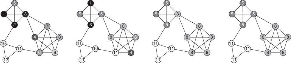
Figure 5.1 Label propagation in a small network with three communities. The labels and shades of the nodes represent community assignments at different iterations of the label propagation method.
For the sake of simplicity, we describe the basic label propagation framework for the case of detecting communities in simple undirected networks. Consider a network with ![]() nodes and let
nodes and let ![]() denote the set of neighbors of node
denote the set of neighbors of node ![]() . Furthermore, let
. Furthermore, let ![]() be the group assignment or community label of node
be the group assignment or community label of node ![]() which we would like to infer. The label propagation method then proceeds as follows. Initially, the nodes are put into separate groups by assigning a unique label to each node as
which we would like to infer. The label propagation method then proceeds as follows. Initially, the nodes are put into separate groups by assigning a unique label to each node as ![]() . Then, the labels are propagated between the nodes until an equilibrium is reached. At every iteration of label propagation, each node
. Then, the labels are propagated between the nodes until an equilibrium is reached. At every iteration of label propagation, each node ![]() adopts the label shared by most of its neighbors,
adopts the label shared by most of its neighbors, ![]() . Hence,
. Hence,
Due to having numerous edges within communities, relative to the number of edges towards the rest of the network, the nodes of a community form a consensus on some label after only a couple of iterations of label propagation. More precisely, in the first few iterations, the labels form small groups in dense regions of the network, which then expand until they reach the borders of communities. Thus, when the propagation converges, meaning that Equation 5.1 holds for all of the nodes and the labels no longer change, connected groups of nodes sharing the same label are classified as communities. Figure 5.1 demonstrates the label propagation method on a small network, where it correctly identifies the three communities in just three iterations. In fact, due to the extremely fast structural inference of label propagation, the estimated number of iterations in a network with a billion edges is about 100 [59].
Label propagation is not limited to simple networks having, at most, one edge between each pair of nodes. Let ![]() be the adjacency matrix of a network, where
be the adjacency matrix of a network, where ![]() is the number of edges between nodes
is the number of edges between nodes ![]() and
and ![]() , and
, and ![]() is the number of self-edges or loops on node
is the number of self-edges or loops on node ![]() . The label propagation rule in Equation 5.1 can be written as
. The label propagation rule in Equation 5.1 can be written as
where ![]() is the Kronecker delta operator that equals one when its arguments are the same and zero otherwise. Furthermore, in weighted or valued networks, the label propagation rule becomes
is the Kronecker delta operator that equals one when its arguments are the same and zero otherwise. Furthermore, in weighted or valued networks, the label propagation rule becomes

where ![]() is the sum of weights on the edges between nodes
is the sum of weights on the edges between nodes ![]() and
and ![]() , and
, and ![]() is the sum of weights on the loops on node
is the sum of weights on the loops on node ![]() . Label propagation can also be adopted for multipartite and other types of networks, which is presented in Section 5.4. However, there seems to be no obvious extension of label propagation to networks with directed arcs, since propagating the labels exclusively in the direction of arcs enables the exchange of labels only between mutually reachable nodes.
. Label propagation can also be adopted for multipartite and other types of networks, which is presented in Section 5.4. However, there seems to be no obvious extension of label propagation to networks with directed arcs, since propagating the labels exclusively in the direction of arcs enables the exchange of labels only between mutually reachable nodes.

Figure 5.2 Resolution of ties between the maximal labels of the central nodes of the networks. The labels and shades of the nodes represent their current community assignments.
5.1.1 Resolution of Label Ties
At each step of label propagation, a node adopts the label shared by most of its neighbors denoted by the maximal label. There can be multiple maximal labels as shown on the left-hand side of Figure 5.2. In that case, the node chooses one maximal label uniformly at random [50]. Note, however, that the propagation might never converge, especially when there are many nodes with multiple maximal labels in their neighborhoods. This is because their labels could constantly change and label convergence would never be reached. The problem is particularly apparent in networks of collaborations between the authors of scientific papers, where a single author often collaborates with others in different research communities.
The simplest solution is always to select the smallest or the largest maximal label according to some predefined ordering [18], which has obvious drawbacks. Leung et al. [35] proposed a seemingly elegant solution to include also the concerned node's label itself into the maximal label consideration in Equation 5.2. This is equivalent to adding a loop on each node in a network. Nevertheless, the label inclusion strategy might actually create ties when there is only one maximal label in a node's neighborhood, which happens in the case of the central node of the network in the middle of Figure 5.2.
Most label propagation algorithms implement the label retention strategy introduced by Barber and Clark [5]. When there are multiple maximal labels in a node's neighborhood, and one of these labels is the current label of the node, the node retains its label. Otherwise, a random maximal label is selected to be the new node label. The main difference to the label inclusion strategy is that the current label of a node is considered only when there actually exist multiple maximal labels in its neighborhood. For example, the network on the right-hand side of Figure 5.2 is at equilibrium under the label retention strategy.
Random resolution of label ties represents the first of two sources of randomness in the label propagation method, hindering its robustness and consequently also the stability of the identified communities. The second is the random order of label propagation.
5.1.2 Order of Label Propagation
The discussion above assumed that, at every iteration of label propagation, all nodes update their labels simultaneously. This is called synchronous propagation [50]. The authors of the original method noticed that synchronous propagation can lead to oscillations of some labels in certain networks. Consider a bipartite or two-mode network with two types of nodes and edges only between the nodes of different type. Assume that, at some iteration of label propagation, the nodes of each type share the same label as in the example on the left-hand side of Figure 5.3. Then, at the next iteration, the labels of the nodes would merely switch and start to oscillate between two equivalent label configurations. For instance, such behavior occurs in networks with star-like communities consisting of one or few central hub nodes that are connected to many peripheral nodes, while the peripheral nodes themselves are not directly connected. Note that label oscillations are not limited to bipartite or nearly bipartite networks [18], as seen in the example on the right-hand side of Figure 5.3.
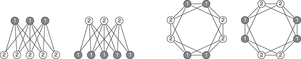
Figure 5.3 Label oscillations in bipartite and non-bipartite networks. The labels and shades of the nodes represent community assignments at two consecutive iterations of the label propagation method.
For this reason, most label propagation algorithms implement asynchronous propagation [50]. At every iteration of label propagation, the labels of the nodes are no longer updated all together, but sequentially in some random order, which is different for each iteration. This is in contrast to synchronous propagation, which always considers the labels from the previous iteration. Due to the random order of label updates, asynchronous propagation successfully breaks the cyclic oscillations of labels in Figure 5.3.
It must be stressed that asynchronous propagation with random tie resolution makes the label propagation method very unstable. In the case of the famous Zachary karate club network [76], the method identifies more than 500 different community structures [65], although the network consists of only 34 nodes. Asynchronous propagation applied to large online social networks and web graphs can wrongly also produce a giant community occupying the majority of the nodes in a network [35].
5.1.3 Label Equilibrium Criterium
Raghavan et al. [50] defined the convergence of label propagation as the state of label equilibrium when Equation 5.1 is satisfied for every node in a network. Let ![]() denote the number of neighbors of node
denote the number of neighbors of node ![]() and let
and let ![]() be the number of neighbors that share label
be the number of neighbors that share label ![]() . The label propagation rule in Equation 5.1 can be rewritten as
. The label propagation rule in Equation 5.1 can be rewritten as
The label equilibrium criterium thus requires that, for every node ![]() , the following must hold
, the following must hold
In other words, all nodes must be labeled with the maximal labels in their neighborhoods.
This criterion is similar, but not equivalent, to the definition of a strong community [49]. Strong communities require that every node has strictly more neighbors in its own community than in all other communities together, whereas at the label equilibrium every node has at least as many neighbors in its own community than in any other community.
An alternative approach is to define the convergence of label propagation as the state when the labels no longer change [5]. Equation 5.5 obviously holds for every node in a network and the label equilibrium is reached. Note, however, that this criterion must necessarily be combined with an appropriate label tie resolution strategy in order to ensure convergence when there are multiple maximal labels in the neighborhoods of nodes.
5.1.4 Algorithm and Complexity
As mentioned in the introduction, the label propagation method can be implemented with a few lines of programming code. Algorithm 5.1 shows the pseudocode of the basic asynchronous propagation framework defining the convergence of label propagation as the state of no label change and implements the retention strategy for label tie resolution.

When the state of label equilibrium is reached, groups of nodes sharing the same label are classified as communities. These can, in general, be disconnected, which happens when a node propagates its label to two or more disconnected nodes, but is itself relabeled in the later iterations of label propagation. Since connectedness is a fundamental property of network communities [23], groups of nodes with the same label are split into connected groups of nodes at the end of label propagation. Reported communities are thus connected components of the subnetworks induced by different node labels.
The label propagation method exhibits near-linear time complexity in the number of edges of a network denoted with ![]() [35,50]. At every iteration of label propagation, the label of node
[35,50]. At every iteration of label propagation, the label of node ![]() can be updated with a sweep through its neighborhood which has complexity
can be updated with a sweep through its neighborhood which has complexity ![]() , where
, where ![]() is the degree of node
is the degree of node ![]() . Since
. Since ![]() , the complexity of an entire iteration of label propagation is
, the complexity of an entire iteration of label propagation is ![]() . A random order or permutation of nodes before each iteration of asynchronous propagation can be computed in
. A random order or permutation of nodes before each iteration of asynchronous propagation can be computed in ![]() time, while the division into connected groups of nodes at the end of label propagation can be implemented with a simple network traversal, which has complexity
time, while the division into connected groups of nodes at the end of label propagation can be implemented with a simple network traversal, which has complexity ![]() .
.
The overall time complexity of label propagation is therefore ![]() , where
, where ![]() is the number of iterations before convergence. In the case of networks with a clear community structure, label propagation commonly converges in no more than ten iterations. Still, the number of iterations increases with the size of a network, as can be seen in Figure 5.4. Šubelj and Bajec [59] estimated the number of iterations of asynchronous label propagation from a large number of empirical networks, obtaining
is the number of iterations before convergence. In the case of networks with a clear community structure, label propagation commonly converges in no more than ten iterations. Still, the number of iterations increases with the size of a network, as can be seen in Figure 5.4. Šubelj and Bajec [59] estimated the number of iterations of asynchronous label propagation from a large number of empirical networks, obtaining ![]() . The time complexity of label propagation is thus approximately
. The time complexity of label propagation is thus approximately ![]() , which makes the method applicable to networks with up to hundreds of millions of nodes and edges on a standard desktop computer as long as the network fits into its main memory.
, which makes the method applicable to networks with up to hundreds of millions of nodes and edges on a standard desktop computer as long as the network fits into its main memory.
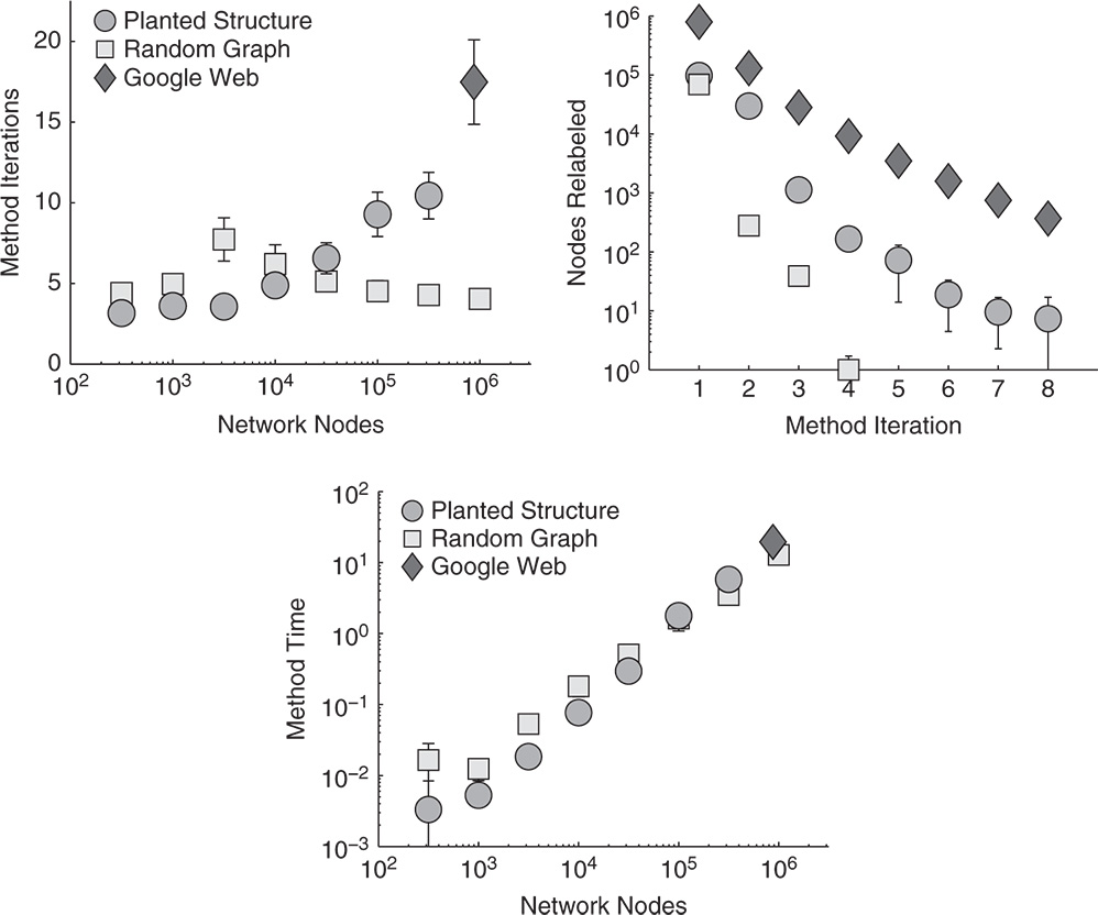
Figure 5.4 The number of iterations of label propagation, the number of relabeled nodes at the first eight iterations, and the running time in seconds. The markers are averages over 25 runs of the label propagation method, while the error bars show standard deviation.
The left-hand side of Figure 5.4 shows the number of iterations of the label propagation framework in Algorithm 5.1 in artificial networks with planted community structure [33], Erdős–Rényi random graphs [22], and a part of the Google web graph [34] available at KONECT.1 The web graph consists of ![]() nodes and
nodes and ![]() edges, while the sizes of random graphs and artificial networks can be seen in Figure 5.4. In random graphs having no structure, label propagation correctly classifies all nodes into a single group in about five iterations, regardless of the size of a graph. Yet, the number of iterations increases with the size in artificial networks with community structure, while the estimated number of iterations in a network with a billion edges is 113 [59].
edges, while the sizes of random graphs and artificial networks can be seen in Figure 5.4. In random graphs having no structure, label propagation correctly classifies all nodes into a single group in about five iterations, regardless of the size of a graph. Yet, the number of iterations increases with the size in artificial networks with community structure, while the estimated number of iterations in a network with a billion edges is 113 [59].
Most nodes acquire their final label after the first few iterations of label propagation. The middle of Figure 5.4 shows the number of nodes that update their label at a particular iteration for the Google web graph, artificial networks having a planted community structure and random graphs with ![]() nodes. The number of relabeled nodes drops exponentially with the number of iterations (logarithmic scales are used). For example, the percentages of relabeled nodes of the web graph after the first five iterations are
nodes. The number of relabeled nodes drops exponentially with the number of iterations (logarithmic scales are used). For example, the percentages of relabeled nodes of the web graph after the first five iterations are ![]() ,
, ![]() ,
, ![]() ,
, ![]() , and
, and ![]() , respectively. Furthermore, the algorithm running time is only 19.5 seconds, as shown on the right-hand side of Figure 5.4.
, respectively. Furthermore, the algorithm running time is only 19.5 seconds, as shown on the right-hand side of Figure 5.4.
5.2 Label Propagation as Optimization
Here, we discuss the objective function of the label propagation method to shed light on label propagation as an optimization method.
At every iteration of label propagation each node adopts the most common label in its neighborhood. Therefore, label propagation can be seen as a local optimization method seeking to maximize the number of neighbors with the same label or, equivalently, minimize the number of neighbors with different labels. From the perspective of node ![]() , the label propagation rule in Equation 5.2 assigns its group label
, the label propagation rule in Equation 5.2 assigns its group label ![]() to maximize
to maximize ![]() , where
, where ![]() is the adjacency matrix of the network. Hence, the objective function maximized by the basic label propagation method is
is the adjacency matrix of the network. Hence, the objective function maximized by the basic label propagation method is

where ![]() is the group labeling of network nodes [5,65]. Notice that
is the group labeling of network nodes [5,65]. Notice that ![]() is non-negative and has the optimum of
is non-negative and has the optimum of ![]() , where
, where ![]() is the number of edges in a network.
is the number of edges in a network.
Equation 5.6 has a trivial optimal solution of labeling all nodes in a network with the same label, corresponding to putting all nodes into one group. Equation 5.2 then holds for every node and ![]() . However, starting with each node in its own group by assigning them unique labels when
. However, starting with each node in its own group by assigning them unique labels when ![]() , the label propagation process usually is trapped in a local optimum. For networks having a clear community structure, this corresponds to nodes of each community being labeled with the same label when
, the label propagation process usually is trapped in a local optimum. For networks having a clear community structure, this corresponds to nodes of each community being labeled with the same label when ![]() , where
, where ![]() is the number of edges between communities. For example, the value of
is the number of edges between communities. For example, the value of ![]() for the community structure revealed on the right-hand side of Figure 5.1 is
for the community structure revealed on the right-hand side of Figure 5.1 is ![]() .
.
Network community structure is only a local optimum of the label propagation process, whereas the global optimal solution corresponds to a trivial, undesirable, labeling. Thus, directly optimizing the objective function of label propagation with some other optimization method trying to escape a local optimum might not yield a favorable outcome. Furthermore, a network can have also many local optima that imply considerably different community structures. As already mentioned in Section 5.1.2, label propagation identifies more than 500 different structures in the Zachary karate club network [76] with 34 nodes and more than ![]() in the Saccharomyces cerevisiae protein interaction network [31] with 2111 nodes [65]. Raghavan et al. [50] suggested aggregating labelings from multiple runs of label propagation. However, this can fragment a network into very small communities [65]. A more suitable method for combining different labelings of label propagation is consensus clustering [24,32,78], but this comes with increased time complexity.
in the Saccharomyces cerevisiae protein interaction network [31] with 2111 nodes [65]. Raghavan et al. [50] suggested aggregating labelings from multiple runs of label propagation. However, this can fragment a network into very small communities [65]. A more suitable method for combining different labelings of label propagation is consensus clustering [24,32,78], but this comes with increased time complexity.
The above perspective on label propagation as an optimization method results from the following equivalence. Tibély and Kertész [65] have shown that the label propagation in Equation 5.2 is equivalent to a ferromagnetic Potts model [48,70]. The ![]() -state Potts model is a generalization of the Ising model as a system of interacting spins on a lattice, with each spin pointing to one of
-state Potts model is a generalization of the Ising model as a system of interacting spins on a lattice, with each spin pointing to one of ![]() equally spaced directions. Consider the so-called standard
equally spaced directions. Consider the so-called standard ![]() -state Potts model on a network placing a spin on each node [51]. Let
-state Potts model on a network placing a spin on each node [51]. Let ![]() denote the spin on node
denote the spin on node ![]() which can be in one of
which can be in one of ![]() possible states, where
possible states, where ![]() is set equal to the number of nodes in a network
is set equal to the number of nodes in a network ![]() . The zero-temperature kinetics of the model are defined as follows. One starts with each spin in its own state as
. The zero-temperature kinetics of the model are defined as follows. One starts with each spin in its own state as ![]() and then iteratively aligns the spins to the states of their neighbors as in the label propagation process. The ground state is ferromagnetic with all spins in the same state, while the dynamics can also get trapped at a metastable state with more than one spin state. The Hamiltonian of the model can be written as
and then iteratively aligns the spins to the states of their neighbors as in the label propagation process. The ground state is ferromagnetic with all spins in the same state, while the dynamics can also get trapped at a metastable state with more than one spin state. The Hamiltonian of the model can be written as

where ![]() are the states of spins on network nodes. By setting
are the states of spins on network nodes. By setting ![]() , minimizing the described Potts model Hamiltonian
, minimizing the described Potts model Hamiltonian ![]() in Equation 5.7 is equivalent to maximizing the objective function of the label propagation method
in Equation 5.7 is equivalent to maximizing the objective function of the label propagation method ![]() in Equation 5.6.
in Equation 5.6.
As is almost any other clustering method, the label propagation method is nondeterministic and can produce different outcomes on different runs. Therefore, throughout the chapter, we report the results obtained over multiple runs of the method.
5.3 Advances of Label Propagation
Section 5.1 presented the basic label propagation method and discussed details of its implementation. Section 5.2 clarified the objective function of label propagation. In this section, we review different advances of the original method, addressing some of the weaknesses identified in the previous sections. Section 5.3.1 shows how to redefine the method's objective function by imposing constraints to use label propagation as a general optimization framework. Section 5.3.2 demonstrates different heuristic approaches changing the method's objective function implicitly by adjusting the propagation strength of individual nodes. This promotes the propagation of labels from certain desirable nodes or, equivalently, suppresses the propagation from the remaining nodes. Finally, Section 5.3.3 discusses different empirically motivated techniques to improve the overall performance of the method.
Unless explicitly stated otherwise, the above advances are presented for the case of non-overlapping community detection in simple undirected networks. Nevertheless, Section 5.4 presents extensions of label propagation to other types of networks such as multipartite, multilayer, and signed networks. Furthermore, in Section 5.5, we show how label propagation can be adopted to detect alternative types of groups such as overlapping or hierarchical communities and groups of nodes that are similarly connected to the rest of the network by structurally equivalent nodes as in Chapter 6. Note that different approaches and techniques described in Sections 5.3–5.5 can be combined. The advances of the basic label propagation method described in this section can be used directly with the extensions to other types of groups and networks described in the next sections.
5.3.1 Label Propagation Under Constraints
As shown in Section 5.2, the objective function of label propagation has a trivial optimal solution of assigning all nodes to a single group. A standard approach for eliminating such undesirable solutions is to add constraints to the objective function of the method. Let ![]() be the objective function of label propagation expressed in the form of the ferromagnetic Potts model Hamiltonian as in Equation 5.7. The modified objective function minimized by label propagation under constraints is
be the objective function of label propagation expressed in the form of the ferromagnetic Potts model Hamiltonian as in Equation 5.7. The modified objective function minimized by label propagation under constraints is ![]() , where
, where ![]() represents a penalty term with imposed constraints with
represents a penalty term with imposed constraints with ![]() being a regularization parameter weighing the penalty term
being a regularization parameter weighing the penalty term ![]() against the original objective function
against the original objective function ![]() .
.
Barber and Clark [5] proposed a penalty term ![]() borrowed from the graph partitioning literature requiring that nodes are divided into smaller groups of the same size:
borrowed from the graph partitioning literature requiring that nodes are divided into smaller groups of the same size:
where ![]() is the number of nodes in group
is the number of nodes in group ![]() ,
, ![]() is the group label of node
is the group label of node ![]() , and
, and ![]() is the number of nodes in a network. The penalty term
is the number of nodes in a network. The penalty term ![]() has the minimum of
has the minimum of ![]() when all nodes are in their own groups and the maximum of
when all nodes are in their own groups and the maximum of ![]() when all nodes are in a single group, which effectively guards against the undesirable trivial solution. The modified objective function
when all nodes are in a single group, which effectively guards against the undesirable trivial solution. The modified objective function ![]() can be written as
can be written as

where ![]() is the adjacency matrix of a network. Equation 5.9 is known as the constant Potts model [67] and is equivalent to a specific version of the stochastic block model [77], while the regularization parameter
is the adjacency matrix of a network. Equation 5.9 is known as the constant Potts model [67] and is equivalent to a specific version of the stochastic block model [77], while the regularization parameter ![]() can be interpreted as the threshold between the density of edges within and between different groups. The label propagation rule in Equations 5.2 and 5.4 for the modified objective function
can be interpreted as the threshold between the density of edges within and between different groups. The label propagation rule in Equations 5.2 and 5.4 for the modified objective function ![]() is
is

where ![]() is the number of neighbors of node
is the number of neighbors of node ![]() in group
in group ![]() . Equation 5.10 can be efficiently implemented with Algorithm 5.1 by updating
. Equation 5.10 can be efficiently implemented with Algorithm 5.1 by updating ![]() .
.
An alternative penalty term ![]() , which has been popular in the community detection literature, requires nodes being divided into groups having the same total degree [5]:
, which has been popular in the community detection literature, requires nodes being divided into groups having the same total degree [5]:

where ![]() is the sum of degrees of nodes in group
is the sum of degrees of nodes in group ![]() and
and ![]() is the degree of node
is the degree of node ![]() . The penalty term
. The penalty term ![]() is again minimized when all nodes are in their own groups and maximized when all nodes are in a single group, avoiding the trivial solution. The modified objective function
is again minimized when all nodes are in their own groups and maximized when all nodes are in a single group, avoiding the trivial solution. The modified objective function ![]() can be written as
can be written as

while the corresponding label propagation rule is

Equation 5.13 can be efficiently implemented with Algorithm 5.1 by updating ![]() .
.
Equation 5.12 is a special case of the Potts model investigated by Reichardt and Bornholdt [51] and is a generalization of a popular quality function in community detection named modularity [45]. The modularity ![]() measures the number of edges within network communities against the expected number of edges in a random graph with the same degree sequence [46]. Formally,
measures the number of edges within network communities against the expected number of edges in a random graph with the same degree sequence [46]. Formally,
Notice that setting ![]() in Equation 5.12 yields
in Equation 5.12 yields ![]() [5].
[5].
Label propagation under the constraints of Equation 5.13 can be employed for maximizing the modularity ![]() . Note, however, that the method might easily get trapped at a local optimum, not corresponding to very high
. Note, however, that the method might easily get trapped at a local optimum, not corresponding to very high ![]() . For example, the average
. For example, the average ![]() over 25 runs for the Google web graph from Figure 5.4 is 0.763. In contrast, the unconstrained label propagation gives a value of 0.801. For this reason, label propagation under constraints is usually combined with a multistep greedy agglomerative algorithm [55], one driving the method away from a local optimum. Using such an optimization framework, Liu and Murata [38] revealed community structures with the highest values of
over 25 runs for the Google web graph from Figure 5.4 is 0.763. In contrast, the unconstrained label propagation gives a value of 0.801. For this reason, label propagation under constraints is usually combined with a multistep greedy agglomerative algorithm [55], one driving the method away from a local optimum. Using such an optimization framework, Liu and Murata [38] revealed community structures with the highest values of ![]() ever reported for some commonly analyzed empirical networks. Han et al. [28] recently adapted the same framework also for another popular quality function called map equation [53].
ever reported for some commonly analyzed empirical networks. Han et al. [28] recently adapted the same framework also for another popular quality function called map equation [53].
The third variant of label propagation under constraints [13] is based on the absolute Potts model [52] with the modified objective function ![]() written as
written as

By setting ![]() in Equation 5.9, one derives
in Equation 5.9, one derives ![]() , implying the method is in fact equivalent to the constant Potts model [67].
, implying the method is in fact equivalent to the constant Potts model [67].
5.3.2 Label Propagation with Preferences
Leung et al. [35] have shown that adjusting the propagation strength of individual nodes can improve the performance of the label propagation method in certain networks. Let ![]() be the propagation strength associated with node
be the propagation strength associated with node ![]() called the node preference. Incorporating the node preferences
called the node preference. Incorporating the node preferences ![]() into the basic label propagation rule in Equation 5.2 gives
into the basic label propagation rule in Equation 5.2 gives
while the method objective function in Equation 5.7 becomes
In contrast to Section 5.3.1, these node preferences impose constraints on the objective function only implicitly by either promoting or suppressing the propagation of labels from certain desirable nodes, as shown in the examples below.
An obvious choice is to set the node preferences equal to the degrees of the nodes as ![]() [35]. For instance, this improves the performance of community detection in networks with high degree nodes in the center of each community. Šubelj and Bajec [57,59] proposed estimating the most central nodes of each community or group during the label propagation process using a random walk diffusion. Consider a random walker utilized on a network limited to the nodes of group
[35]. For instance, this improves the performance of community detection in networks with high degree nodes in the center of each community. Šubelj and Bajec [57,59] proposed estimating the most central nodes of each community or group during the label propagation process using a random walk diffusion. Consider a random walker utilized on a network limited to the nodes of group ![]() and let
and let ![]() be the probability that the walker visits node
be the probability that the walker visits node ![]() . The probabilities
. The probabilities ![]() are high for the most central nodes of group
are high for the most central nodes of group ![]() and low for the nodes on the border. It holds that
and low for the nodes on the border. It holds that

where ![]() is the number of neighbors of node
is the number of neighbors of node ![]() in its group
in its group ![]() . Clearly
. Clearly ![]() is the solution of Equation 5.18, but initializing the probabilities as
is the solution of Equation 5.18, but initializing the probabilities as ![]() and updating their values according to Equation 5.18 only when the nodes change their groups
and updating their values according to Equation 5.18 only when the nodes change their groups ![]() gives a different result. This mimics the actual propagation of labels occurring in a random order and keeps the node probabilities
gives a different result. This mimics the actual propagation of labels occurring in a random order and keeps the node probabilities ![]() synchronized with the node groups
synchronized with the node groups ![]() . Equation 5.18 can be efficiently implemented in Algorithm 5.1 by updating
. Equation 5.18 can be efficiently implemented in Algorithm 5.1 by updating ![]() .
.
Label propagation with node preferences defined in Equation 5.18 is called defensive propagation [59] as it restrains the propagation of labels to preserve a larger number of groups by increasing the propagation strength of their central nodes or, equivalently, decreasing the propagation strength of their border nodes. Another strategy is to increase the propagation strength of the border nodes, which results in a more rapid expansion of groups and a smaller number of larger groups. This is called offensive propagation [59] with the label propagation rule written as
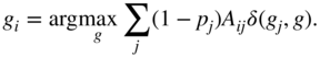
The left-hand side of Figure 5.5 demonstrates the defensive and offensive label propagation methods in an artificial network with two planted communities that are only loosely separated. While defensive propagation correctly identifies the communities planted in the network, offensive propagation spreads the labels beyond the borders of the communities and reveals no structure in this network. The right-hand side of Figure 5.5 compares the methods also on a graph partitioning problem. The methods are applied to a triangular grid with four edges removed, which makes a division into two groups the only sensible partition. In contrast, offensive propagation correctly partitions the grid into two groups, whereas defensive propagation overly restrains the spread of labels and recovers four groups.
Figure 5.5 Comparison of defensive and offensive label propagation in artificial networks with a planted community structure and a triangular grid with four missing edges. The labels and shades of the nodes represent communities or groups identified by the two methods.
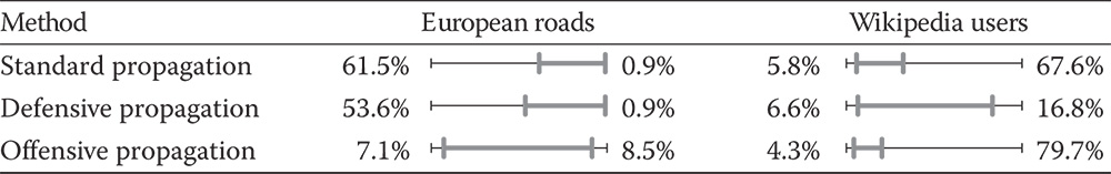
Table 5.1 Degeneracy diagrams of the label propagation methods displaying the non-degenerate ranges of the revealed groups (thick lines), while the percentages show the fraction of nodes in the tiny groups (left) and in the largest group (right). The values are averages over 25 runs of the methods
|
Table 5.1 further compares the defensive and offensive label propagation methods on the European road network [58] with 1174 nodes and a network of user interactions on Wikipedia [43] with ![]() nodes. Both networks are available at KONECT. Degeneracy diagrams in Table 5.1 show the non-degenerate or effective ranges of the revealed groups that span the fraction of nodes not covered by the tiny groups with three nodes or less, or the largest group [64] (left and right percentages, respectively). Ideally, the thick lines in Table 5.1 would span from left to right. Due to the sparse grid-like structure of the road network, defensive propagation partitions
nodes. Both networks are available at KONECT. Degeneracy diagrams in Table 5.1 show the non-degenerate or effective ranges of the revealed groups that span the fraction of nodes not covered by the tiny groups with three nodes or less, or the largest group [64] (left and right percentages, respectively). Ideally, the thick lines in Table 5.1 would span from left to right. Due to the sparse grid-like structure of the road network, defensive propagation partitions ![]() of the nodes into tiny groups, which is not a useful result. This can be avoided by using offensive propagation, where this percentage equals
of the nodes into tiny groups, which is not a useful result. This can be avoided by using offensive propagation, where this percentage equals ![]() . However, in the case of much denser Wikipedia network, offensive propagation returns one giant group occupying
. However, in the case of much denser Wikipedia network, offensive propagation returns one giant group occupying ![]() of the nodes, thus defensive propagation with
of the nodes, thus defensive propagation with ![]() is preferred. Note that the crucial difference between these two networks requiring the use of different methods is their density. A generally applicable approach is first to use defensive propagation and then iteratively refine the revealed groups with offensive propagation [57,59], in this order. For example, such an approach reveals a partition of the road network with
is preferred. Note that the crucial difference between these two networks requiring the use of different methods is their density. A generally applicable approach is first to use defensive propagation and then iteratively refine the revealed groups with offensive propagation [57,59], in this order. For example, such an approach reveals a partition of the road network with ![]() of the nodes in the tiny groups and
of the nodes in the tiny groups and ![]() of the nodes in the largest group on average.
of the nodes in the largest group on average.
An alternative definition of defensive and offensive label propagation is to replace the random walk diffusion in Equation 5.18 with the eigenvector centrality [14] defined as
where ![]() is a normalizing constant equal to the leading eigenvalue of the adjacency matrix
is a normalizing constant equal to the leading eigenvalue of the adjacency matrix ![]() reduced to the nodes in group
reduced to the nodes in group ![]() . Zhang et al. [77] have shown that defensive label propagation with the eigenvector centrality for the node preferences is equivalent to the maximum likelihood estimation of a stochastic block model with Gaussian weights on the edges. This relates the label propagation method with yet another popular approach in the literature that is more thoroughly described in Chapter 11.
. Zhang et al. [77] have shown that defensive label propagation with the eigenvector centrality for the node preferences is equivalent to the maximum likelihood estimation of a stochastic block model with Gaussian weights on the edges. This relates the label propagation method with yet another popular approach in the literature that is more thoroughly described in Chapter 11.
5.3.3 Method Stability and Complexity
Here, we discuss different techniques to improve the performance of the label propagation method by either increasing its stability or reducing its complexity.
One of the main sources of instability of the method is the random order of label updates in asynchronous propagation [35,50]. Recall that the primary reason for this is to break cyclic oscillations of labels in synchronous propagation as it occurs in Figure 5.3. Li et al. [36] also proposed to use synchronous propagation even though this can lead to oscillations of labels, but to break the oscillations by making the label propagation rule in Equation 5.2 probabilistic. The probability that the node ![]() with group label
with group label ![]() updates its label to
updates its label to ![]() is defined as
is defined as

Although this successfully eliminates the oscillations of labels in Figure 5.3, probabilistic label propagation can make the method even more unstable. It must be stressed that this instability represents a major issue, especially in very large networks.
Cordasco and Gargano [17,18] proposed a more elegant solution called semi-synchronous label propagation based on node coloring. A coloring of network nodes is an assignment of colors to nodes such that no two connected nodes share the same color [44]. Notice that if two nodes are not connected their labels do not directly depend on one another in Equation 5.2 and can therefore be updated simultaneously using synchronous propagation. Given a coloring of the network, semi-synchronous propagation traverses different colors in a random order as in asynchronous propagation. In contrast, the labels of the nodes with the same color are updated simultaneously as in synchronous propagation. For instance, coloring each node with a different color is equivalent to asynchronous propagation, while a simple greedy algorithm can find a coloring with at most ![]() colors, where
colors, where ![]() is the maximum degree in a network. In contrast to synchronous and asynchronous propagation, the convergence of semi-synchronous propagation can be formally proven.
is the maximum degree in a network. In contrast to synchronous and asynchronous propagation, the convergence of semi-synchronous propagation can be formally proven.
Šubelj and Bajec [58,61] observed empirically that updating the labels of the nodes in some fixed order drives the label propagation process towards similar solutions as setting the node preferences in Equation 5.16 higher (lower) for the nodes that appear earlier (later) in the order and then updating their labels in a random order as in asynchronous propagation. The node preferences can thus be used as node balancers to counteract the randomness introduced by asynchronous propagation. Let ![]() be a normalized position of the node
be a normalized position of the node ![]() in some random order, which is set to
in some random order, which is set to ![]() for the first node,
for the first node, ![]() for the second node and so on, where
for the second node and so on, where ![]() is the number of nodes in a network. The value
is the number of nodes in a network. The value ![]() represents the time at which the label of node
represents the time at which the label of node ![]() is updated. Balanced label propagation sets the node preferences using a logistic function as
is updated. Balanced label propagation sets the node preferences using a logistic function as

where ![]() is a parameter of the method. For
is a parameter of the method. For ![]() , Equation 5.22 is equivalent to the standard label propagation rule in Equation 5.2, while
, Equation 5.22 is equivalent to the standard label propagation rule in Equation 5.2, while ![]() makes the method more stable, but this increases its time complexity. In practice, one must therefore decide on a compromise between the method stability and its time complexity.
makes the method more stable, but this increases its time complexity. In practice, one must therefore decide on a compromise between the method stability and its time complexity.
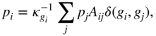
The method stability is tightly knit with its performance. Figure 5.6 compares community detection of the label propagation methods in artificial networks with four planted communities [25]. Community structure is controlled by a mixing parameter ![]() that represents the fraction of nodes' neighbors in their own community. For example, the left-hand side of Figure 5.6 shows realizations of networks for
that represents the fraction of nodes' neighbors in their own community. For example, the left-hand side of Figure 5.6 shows realizations of networks for ![]() and 0.4. Performance of the methods is measured with the normalized mutual information [23], where higher is better (see [23] for the exact definition). As seen in the right-hand side of Figure 5.6, balanced label propagation combined with the defensive node preferences in Equation 5.18 performs best in these networks, when
and 0.4. Performance of the methods is measured with the normalized mutual information [23], where higher is better (see [23] for the exact definition). As seen in the right-hand side of Figure 5.6, balanced label propagation combined with the defensive node preferences in Equation 5.18 performs best in these networks, when ![]() .
.
Another prominent approach for improving community detection of the label propagation methods is consensus clustering [24,32,78]. One first applies the method to a given network multiple times and constructs a weighted consensus graph, where weights represent the number of times two nodes are classified into the same community. Note that only edges with weights above a given threshold are kept. The entire process is then repeated on the consensus graph until the revealed communities no longer change. For example, the left-hand side of Figure 5.7 shows two realizations of groups obtained with the standard label propagation method in Equation 5.2 in artificial networks for ![]() . Although these do not exactly coincide with the planted communities, label propagation in the corresponding consensus graph recovers the correct community structure as demonstrated on the right-hand side of Figure 5.7. For another example, Figure 5.8 shows the largest connected component of the European road network from Table 5.1 and the largest groups revealed by the offensive label propagation method in Equation 5.19 with 25 runs of consensus clustering.
. Although these do not exactly coincide with the planted communities, label propagation in the corresponding consensus graph recovers the correct community structure as demonstrated on the right-hand side of Figure 5.7. For another example, Figure 5.8 shows the largest connected component of the European road network from Table 5.1 and the largest groups revealed by the offensive label propagation method in Equation 5.19 with 25 runs of consensus clustering.
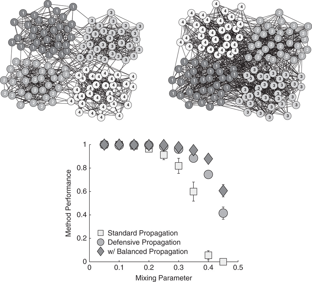
Figure 5.6 Performance of the label propagation methods in artificial networks with planted community structure represented by the labels and shades of the nodes. The markers are averages over 25 runs of the methods, while the error bars show standard errors.
Note, however, that consensus clustering can substantially increase the method's computational time. Other work has thus considered different hybrid approaches to improve the stability of community detection of the label propagation methods, where community structure revealed by one method is refined by another [57,59], possibly proceeding iteratively or incrementally [19,35]. For instance, label propagation under constraints [28,38] has traditionally been combined with a multistep greedy agglomeration [55].
In the remaining sections, we also briefly discuss different approaches to reduce the complexity of the label propagation method. Although the time complexity is already nearly linear ![]() , where
, where ![]() is the number of edges in a network [59], one can still further improve the computational time. As shown in Figure 5.4, the number of nodes that update their label at a particular iteration of label propagation drops exponentially with the number of iterations. Thus, after a couple of iterations, most nodes have already acquired their final label and no longer need to be updated. For instance, one can selectively update only the labels of those nodes for which the fraction of neighbors sharing the same label is below a certain threshold [35], which can make the method truly linear
is the number of edges in a network [59], one can still further improve the computational time. As shown in Figure 5.4, the number of nodes that update their label at a particular iteration of label propagation drops exponentially with the number of iterations. Thus, after a couple of iterations, most nodes have already acquired their final label and no longer need to be updated. For instance, one can selectively update only the labels of those nodes for which the fraction of neighbors sharing the same label is below a certain threshold [35], which can make the method truly linear ![]() . Xie and Szymanski [72] further formalized this idea using the concept of active and passive nodes. A node is said to be passive if updating would not change its label. Otherwise, the node is active. The labels are therefore propagated only between the active nodes until all nodes become passive.
. Xie and Szymanski [72] further formalized this idea using the concept of active and passive nodes. A node is said to be passive if updating would not change its label. Otherwise, the node is active. The labels are therefore propagated only between the active nodes until all nodes become passive.
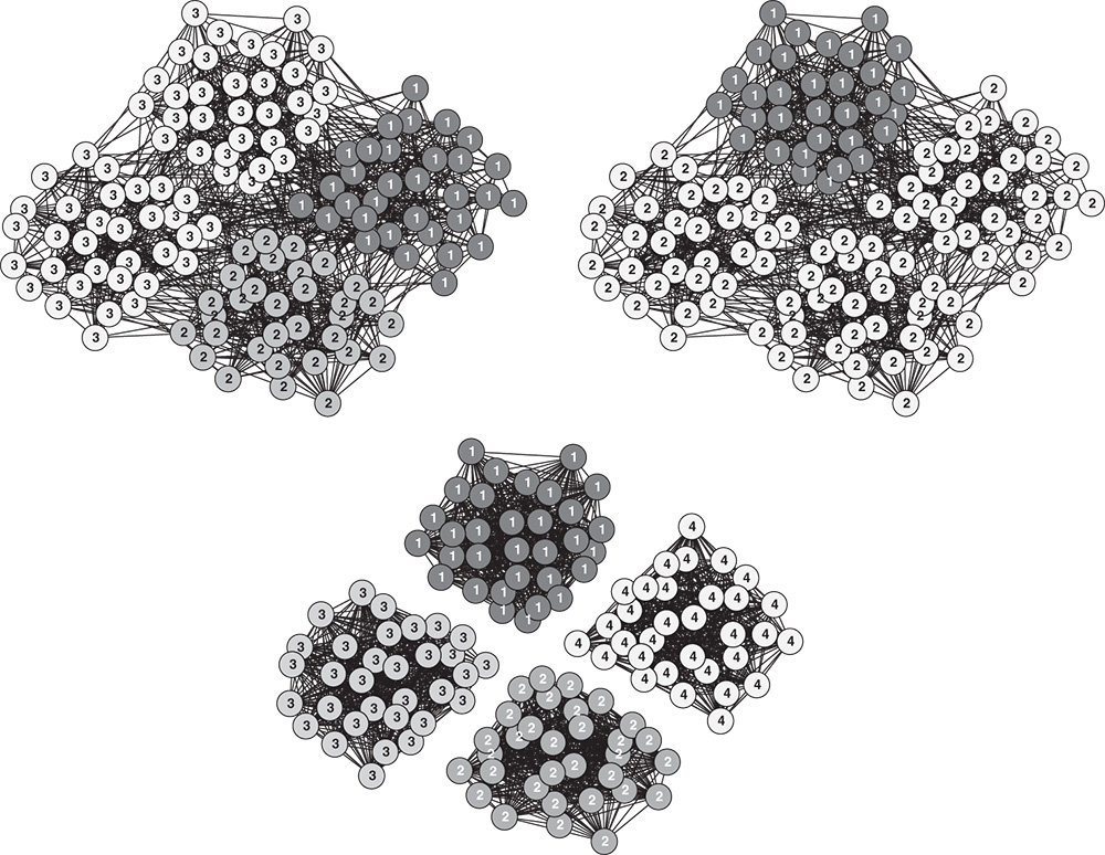
Figure 5.7 Label propagation in artificial networks with planted community structure and the corresponding consensus graph. The labels and shades of the nodes represent communities identified by the label propagation method.
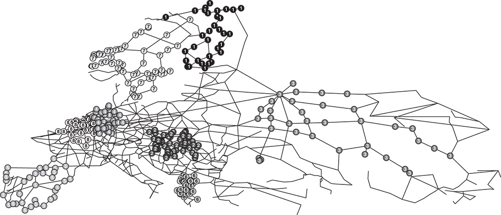
Figure 5.8 Offensive label propagation with consensus clustering in the European road network. The labels and shades of the nodes represent the largest eight groups identified by the method.
Due to its algorithmic simplicity, the label propagation method is easily parallelizable, especially with synchronous or semi-synchronous propagation mentioned above. The method is thus suitable for application in distributed computing environments such as Spark2 [16] or Hadoop3 [47] and on parallel architectures [56]. In this way, label propagation has been successfully used on billion-node networks [16,69].
5.4 Extensions to Other Networks
Throughout the chapter, we have assumed that the label propagation method is applied to simple undirected networks. Nevertheless, the method can easily be extended to networks with multiple edges between the nodes as in Equation 5.2 and networks with weights on the edges as in Equation 5.3. This holds also for the different advances of the propagation methods presented in Section 5.3. In contrast, there seems to be no straightforward extension to networks with directed arcs. The reason for this is that propagating the labels exclusively in the direction of arcs enables exchange of labels only between mutually reachable nodes forming a strongly connected component. Since any directed network is a directed acyclic graph on its strongly connected components, the labels can propagate between the nodes of different strongly connected components merely in one direction. Therefore, one usually disregards the directions of arcs when applying the label propagation method to directed networks except in the case when most arcs are reciprocal.
The method can be extended to signed networks with positive and negative edges between the nodes, as in the approach of Doreian and Mrvar [20]. In order to partition the network in such a way that positive edges mostly appear within the groups and negative edges between the groups, one assigns some fixed positive (negative) weight to positive (negative) edges and then applies the standard label propagation method for weighted networks in Equation 5.3. According to the objective function in Equation 5.7, the method thus simultaneously tries to maximize the number of positive edges within the groups and the number of negative edges between the groups. Still, this does not ensure that the nodes connected by a negative edge are necessarily assigned to different groups, but merely restricts the propagation of labels along the negative edges [1].
Table 5.2 shows the standard and signed label propagation methods applied to the Wikipedia web of trust network [43] available at KONECT. The network consists of ![]() nodes connected by
nodes connected by ![]() positive edges and
positive edges and ![]() negative edges. Standard label propagation ignoring the signs of edges reveals one giant group occupying
negative edges. Standard label propagation ignoring the signs of edges reveals one giant group occupying ![]() of the nodes on average. Most positive edges are thus obviously within the groups, but the same also holds for negative edges. Signed label propagation with positive and negative weights on the edges reduces the size of the largest group to
of the nodes on average. Most positive edges are thus obviously within the groups, but the same also holds for negative edges. Signed label propagation with positive and negative weights on the edges reduces the size of the largest group to ![]() of the nodes on average. Most positive edges remain within the groups, while more than half of negative edges are between the groups. Note that the method assigns weights 1 and
of the nodes on average. Most positive edges remain within the groups, while more than half of negative edges are between the groups. Note that the method assigns weights 1 and ![]() to positive and negative edges. Since only
to positive and negative edges. Since only ![]() of the edges in the network are negative, this actually puts more emphasis on the positive edges. To circumvent the latter, one can assign equal total weight to positive and negative edges by using weights
of the edges in the network are negative, this actually puts more emphasis on the positive edges. To circumvent the latter, one can assign equal total weight to positive and negative edges by using weights ![]() and
and ![]() , where
, where ![]() and
and ![]() are the numbers of positive and negative edges. Signed label propagation with equal total weights returns a larger number of groups with
are the numbers of positive and negative edges. Signed label propagation with equal total weights returns a larger number of groups with ![]() of the nodes in the largest group, and about the same fraction of positive edges within the groups and negative edges between the groups. For further discussion on partitioning signed networks see Chapter 8.
of the nodes in the largest group, and about the same fraction of positive edges within the groups and negative edges between the groups. For further discussion on partitioning signed networks see Chapter 8.
Table 5.2 Comparison of the label propagation methods on the signed Wikipedia web of trust network. The values are averages over ![]() runs of the methods, while
runs of the methods, while ![]() is defined in Equation (5.7)
is defined in Equation (5.7)
| Method | Hamiltonian |
||
| Standard propagation | |||
| Signed propagation | |||
| With equal weights |
Any label propagation method can also be used on bipartite networks with two types of nodes and edges only between the nodes of different type as on the left-hand side of Figure 5.9. For instance, Barber and Clark [5] adopted the label propagation methods under constraints to optimize bipartite modularity [4]. Liu and Murata [39,40] proposed a proper extension of the label propagation framework to bipartite networks. This is a special case of semi-synchronous propagation with node coloring discussed in Section 5.3.3. Recall that semi-synchronous propagation updates the labels of the nodes with the same color synchronously, while different colors are traversed asynchronously. In bipartite networks, the types of the nodes can be taken for their colors, thus the method alternates between the nodes of each type, while the propagation of labels always occurs synchronously. The same principle can be extended also to multipartite networks, where again the nodes of the same type are assigned the same color. However, in multirelational or multilayer networks [11], one can separately consider the nodes of different layers, but the propagation of labels within each layer requires asynchronicity for the method to converge.
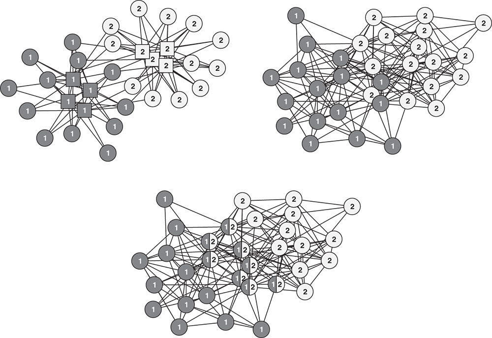
Figure 5.9 Non-overlapping and overlapping label propagation in artificial networks with planted community structure. The labels and shades of the nodes represent communities identified by different methods, while the types of nodes of the bipartite network are shown with distinct symbols.
5.5 Alternative Types of Network Structures
The label propagation method was originally designed to detect non-overlapping communities in networks [35,50]. In the following, we show how the method can be extended to more diverse network structures. We consider extensions to overlapping groups of nodes, groups of nodes at multiple resolutions that form a nested hierarchy, and groups of structurally equivalent nodes. Note that, in contrast to the extensions to other types of networks in Section 5.4, this increases the time complexity of the method derived in Section 5.1.4. As shown in the following, the time complexity increases by a factor depending on the type of groups considered.
5.5.1 Overlapping Groups of Nodes
Extension of the label propagation method to overlapping groups of nodes is relatively straightforward [26,71]. Instead of assigning a single group label ![]() to node
to node ![]() as the standard label propagation method in Equation 5.2, multiple labels are assigned to each node. Let
as the standard label propagation method in Equation 5.2, multiple labels are assigned to each node. Let ![]() be the group function of node
be the group function of node ![]() where
where ![]() represents how strongly the node is affiliated to group
represents how strongly the node is affiliated to group ![]() . In particular, the node belongs to groups
. In particular, the node belongs to groups ![]() for which
for which ![]() , while its group affiliations are normalized to one as
, while its group affiliations are normalized to one as ![]() . At the beginning of label propagation, each node is put into its own group by setting
. At the beginning of label propagation, each node is put into its own group by setting ![]() . Then, at every iteration, each node adopts the group labels of its neighbors. The affiliation
. Then, at every iteration, each node adopts the group labels of its neighbors. The affiliation ![]() of node
of node ![]() to group
to group ![]() is computed as the average affiliation of its neighbors. Hence,
is computed as the average affiliation of its neighbors. Hence,
where ![]() is the network adjacency matrix and
is the network adjacency matrix and ![]() is the degree of node
is the degree of node ![]() . Equation 5.23 can be combined also with an inflation operator raising
. Equation 5.23 can be combined also with an inflation operator raising ![]() to some exponent [74]. Obviously, the groups can now overlap as the nodes can belong to multiple groups. For example, the right-hand side of Figure 5.9 demonstrates the non-overlapping and overlapping label propagation methods in an artificial network with two planted overlapping communities.
to some exponent [74]. Obviously, the groups can now overlap as the nodes can belong to multiple groups. For example, the right-hand side of Figure 5.9 demonstrates the non-overlapping and overlapping label propagation methods in an artificial network with two planted overlapping communities.
Notice, however, that the label propagation rule in Equation 5.23 inevitably leads to every node in a network belonging to all groups. It is therefore necessary to limit the number of groups a single node can belong to. Gregory [26] proposed that, after each iteration of label propagation, the group affiliations ![]() below
below ![]() are set to zero and renormalized, where
are set to zero and renormalized, where ![]() is a method parameter. Since
is a method parameter. Since ![]() for every node, the nodes can thus belong to at most
for every node, the nodes can thus belong to at most ![]() groups. The parameter
groups. The parameter ![]() can be difficult to determine if a network consists of overlapping and non-overlapping groups. Wu et al. [71] suggested replacing the parameter
can be difficult to determine if a network consists of overlapping and non-overlapping groups. Wu et al. [71] suggested replacing the parameter ![]() by a node-dependent threshold
by a node-dependent threshold ![]() to keep node
to keep node ![]() affiliated to group
affiliated to group ![]() as long as
as long as

The time complexity of the described overlapping label propagation method is ![]() , where
, where ![]() is the number of iterations of label propagation,
is the number of iterations of label propagation, ![]() is the number of edges in a network, and
is the number of edges in a network, and ![]() is the maximum number of groups a single node belongs to. The method is implemented by a popular community detection algorithm COPRA4 [26].
is the maximum number of groups a single node belongs to. The method is implemented by a popular community detection algorithm COPRA4 [26].
It is also possible to detect overlapping groups of nodes by using the standard non-overlapping label propagation method. Xie and Szymanski [73,75] proposed associating a memory with each node to store group labels from previous iterations. Running the label propagation for ![]() iterations assigns
iterations assigns ![]() labels to each node's memory. The probability of observing label
labels to each node's memory. The probability of observing label ![]() in the memory of node
in the memory of node ![]() or, equivalently, the number of occurrences of
or, equivalently, the number of occurrences of ![]() in the memory of
in the memory of ![]() can then be interpreted as the group affiliation
can then be interpreted as the group affiliation ![]() as defined above. Note that label propagation with node memory splits the label propagation rule in Equation 5.2 into two steps. Each neighbor
as defined above. Note that label propagation with node memory splits the label propagation rule in Equation 5.2 into two steps. Each neighbor ![]() of the considered node
of the considered node ![]() first propagates a random label from its memory, with the label
first propagates a random label from its memory, with the label ![]() being selected with probability
being selected with probability ![]() , while node
, while node ![]() then adds the most frequently propagated label to its memory. The time complexity of the method is
then adds the most frequently propagated label to its memory. The time complexity of the method is ![]() , where
, where ![]() is a small constant set to say 25. The method is implemented by another popular community detection algorithm SLPA5 [75] and its successor SpeakEasy6 [24].
is a small constant set to say 25. The method is implemented by another popular community detection algorithm SLPA5 [75] and its successor SpeakEasy6 [24].
DEMON7 [19] is a well-known community detection algorithm that also uses non-overlapping label propagation to detect overlapping groups. Instead of assigning a memory to each node as above, this label propagation method is separately applied to the subnetworks reduced to the neighborhoods of the nodes. All of the resulting groups that are, in general, overlapping are then merged together.
5.5.2 Hierarchy of Groups of Nodes
Label propagation can be applied in a hierarchical manner in order to reveal a nested hierarchy of groups of nodes [35,37,59,62]. The bottom level of such a hierarchy represents groups of nodes. The next level represents groups of groups of nodes and so on. Cutting the hierarchy at different levels results in groups of nodes at multiple resolutions. For example, Figure 5.10 demonstrates the hierarchical label propagation method in artificial networks with two levels of planted community structure. Let ![]() denote the groups revealed by the basic label propagation method in Equation 5.2, which represent the bottom level of the group hierarchy. One then constructs a meta-network, where nodes correspond to different groups
denote the groups revealed by the basic label propagation method in Equation 5.2, which represent the bottom level of the group hierarchy. One then constructs a meta-network, where nodes correspond to different groups ![]() and an edge is put between the groups
and an edge is put between the groups ![]() and
and ![]() if their nodes are connected in the original network. The weight of the edge is set to the number of edges between the groups
if their nodes are connected in the original network. The weight of the edge is set to the number of edges between the groups ![]() and
and ![]() in the original network. Similarly, a loop is added to each group
in the original network. Similarly, a loop is added to each group ![]() with a weight equal to the number of edges within the group
with a weight equal to the number of edges within the group ![]() in the original network. Finally, one applies the weighted label propagation method in Equation 5.3 to the constructed meta-network to reveal groups of groups
in the original network. Finally, one applies the weighted label propagation method in Equation 5.3 to the constructed meta-network to reveal groups of groups ![]() . These constitute the next level of the group hierarchy. The entire process of such bottom-up group agglomeration is repeated iteratively until a single group is recovered, which is the root of the hierarchy. Note that label propagation with group agglomeration is algorithmically equivalent to the famous Louvain modularity optimization method [10,66].
. These constitute the next level of the group hierarchy. The entire process of such bottom-up group agglomeration is repeated iteratively until a single group is recovered, which is the root of the hierarchy. Note that label propagation with group agglomeration is algorithmically equivalent to the famous Louvain modularity optimization method [10,66].

Figure 5.10 Artificial networks with two levels of planted community structure and the corresponding group hierarchy. The labels and shades of the nodes represent communities identified by the label propagation method.
Figure 5.11 shows the meta-networks of the largest connected components of the Google web graph from Figure 5.4 with ![]() nodes and the Pennsylvania road network [34] with
nodes and the Pennsylvania road network [34] with ![]() nodes. Both networks are available at KONECT. The meta-networks were revealed by the hierarchical label propagation method with two and three steps of group agglomeration, and consist of 564 and 235 nodes, respectively. Notice that, although the networks are reduced to less than a thousandth of their original size, the group agglomeration process preserves a dense central core of the web graph and a sparse homogeneous topology of the road network [9].
nodes. Both networks are available at KONECT. The meta-networks were revealed by the hierarchical label propagation method with two and three steps of group agglomeration, and consist of 564 and 235 nodes, respectively. Notice that, although the networks are reduced to less than a thousandth of their original size, the group agglomeration process preserves a dense central core of the web graph and a sparse homogeneous topology of the road network [9].

Figure 5.11 The meta-networks of the Google web graph and the Pennsylvania road network identified by the hierarchical label propagation method. The shades of the nodes are proportional to their corrected clustering coefficient [6], where darker (lighter) means higher (lower).
Bottom-up group agglomeration can be effectively combined with top-down group refinement [62,63]. Let ![]() be the groups revealed at some step of the group agglomeration. Prior to the construction of the meta-network, one separately applies the label propagation method to the subnetworks of the original network limited to the nodes of groups
be the groups revealed at some step of the group agglomeration. Prior to the construction of the meta-network, one separately applies the label propagation method to the subnetworks of the original network limited to the nodes of groups ![]() . As this process repeats recursively until a single group is recovered, a sub-hierarchy of groups is revealed for each group
. As this process repeats recursively until a single group is recovered, a sub-hierarchy of groups is revealed for each group ![]() . Bottom-up agglomeration with top-down refinement enables the identification of a very detailed hierarchy of groups present in a network [24,62]. One can also further control the resolution of groups by adjusting the weights on the loops in the meta-network [27]. The time complexity of the described hierarchical label propagation method is
. Bottom-up agglomeration with top-down refinement enables the identification of a very detailed hierarchy of groups present in a network [24,62]. One can also further control the resolution of groups by adjusting the weights on the loops in the meta-network [27]. The time complexity of the described hierarchical label propagation method is ![]() , where
, where ![]() is the number of iterations and
is the number of iterations and ![]() the number of edges as before, while
the number of edges as before, while ![]() is the number of levels of the group hierarchy.
is the number of levels of the group hierarchy.
5.5.3 Structural Equivalence Groups
The Different label propagation methods presented so far can be used to reveal connected and cohesive groups of nodes in a network. This includes detection of densely connected communities and graph partitioning as demonstrated in Figure 5.5. However, the methods cannot be adopted for detection of any kind of disconnected groups of nodes. Therefore, possibly the most interesting extension of the label propagation method is to find groups of structurally equivalent nodes [42,60–62]. Informally, two nodes are said to be structurally equivalent if they are connected to the same other nodes in the network and thus have the same common neighbors [21,41], whereas the nodes themselves may be connected or not. We here consider a relaxed definition of structural equivalence in which nodes can have only the majority of their neighbors in common. For example, the left-hand side of Figure 5.12 shows an artificial network with two planted communities of nodes labeled with 2 and 4, and two groups of structurally equivalent nodes labeled with 1 and 3 that form a bipartite structure. The former are also called assortative groups, while the latter are referred to as disassortative groups [23].
Let ![]() denote the degree of node
denote the degree of node ![]() and
and ![]() the number of common neighbors of nodes
the number of common neighbors of nodes ![]() and
and ![]() . Hence,
. Hence, ![]() and
and ![]() , where
, where ![]() is the network adjacency matrix. Xie and Szymanski [72] modified the label propagation rule in Equation 5.2 as
is the network adjacency matrix. Xie and Szymanski [72] modified the label propagation rule in Equation 5.2 as
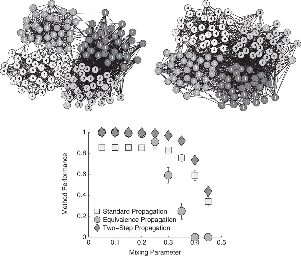
Figure 5.12 Performance of the label propagation methods in artificial networks with planted communities and structural equivalence groups represented by the labels and shades of the nodes. The markers are averages over 25 runs of the methods, while the error bars show standard errors.
which increases the strength of propagation between structurally equivalent nodes. Notice that Equation 5.25 is in fact equivalent to simultaneously propagating the labels between the neighboring nodes as standard and also through their common neighbors represented by the term ![]() . Yet, the labels are propagated merely between connected nodes, thus the method can still reveal only connected groups of nodes.
. Yet, the labels are propagated merely between connected nodes, thus the method can still reveal only connected groups of nodes.
Šubelj and Bajec [61,62] proposed a proper extension of the label propagation method for structural equivalence that separately propagates the labels between the neighboring nodes and through nodes' common neighbors. Let ![]() be a parameter of group
be a parameter of group ![]() that is set close to one for connected groups and close to zero for structural equivalence groups. The label propagation rule for general groups of nodes is then written as
that is set close to one for connected groups and close to zero for structural equivalence groups. The label propagation rule for general groups of nodes is then written as

The left-hand sum propagates the labels between the neighboring nodes ![]() and
and ![]() , while the right-hand sum propagates the labels between the nodes
, while the right-hand sum propagates the labels between the nodes ![]() and
and ![]() through their common neighbors
through their common neighbors ![]() . The degree
. The degree ![]() in the denominator ensures that the number of terms in both sums is proportional to
in the denominator ensures that the number of terms in both sums is proportional to ![]() . By setting all group parameters in Equation 5.26 as
. By setting all group parameters in Equation 5.26 as ![]() , one retrieves the standard label propagation method in Equation 5.2 that can detect connected groups of nodes like communities, while setting
, one retrieves the standard label propagation method in Equation 5.2 that can detect connected groups of nodes like communities, while setting ![]() , the method can detect structural equivalence groups. In the case when a community consists of structurally equivalent nodes as in a clique of nodes, any of the two methods can be used. In practice, the group parameters
, the method can detect structural equivalence groups. In the case when a community consists of structurally equivalent nodes as in a clique of nodes, any of the two methods can be used. In practice, the group parameters ![]() can be inferred from the network structure or estimated during the label propagation process [61,62]. However, this can make the method very unstable. For this reason, we propose a much simpler approach.
can be inferred from the network structure or estimated during the label propagation process [61,62]. However, this can make the method very unstable. For this reason, we propose a much simpler approach.
Applying the standard label propagation method to the network on the left-hand side of Figure 5.12 reveals three groups of nodes, since both structural equivalence groups are detected as a single group of nodes. In general, configurations of connected structural equivalence groups are merged together by the method. One can, however, employ this behavior to detect structural equivalence groups using a two-step approach with top-down group refinement introduced before [62,63]. The first step reveals connected groups of nodes using the standard label propagation method by setting ![]() in Equation 5.26. This includes communities and configurations of connected structural equivalence groups. In the second step, one separately tries to refine each group from the first step using the structural equivalence label propagation method by setting
in Equation 5.26. This includes communities and configurations of connected structural equivalence groups. In the second step, one separately tries to refine each group from the first step using the structural equivalence label propagation method by setting ![]() in Equation 5.26. While communities are still detected as a single group of nodes, configurations of structural equivalence groups are now further partitioned into separate structural equivalence groups.
in Equation 5.26. While communities are still detected as a single group of nodes, configurations of structural equivalence groups are now further partitioned into separate structural equivalence groups.
The right-hand side of Figure 5.12 compares group detection of the label propagation methods in artificial networks with four groups discussed above [61]. Network structure is controlled by a mixing parameter ![]() that represents the fraction of edges that comply with the group structure, while the examples on the left-hand side of Figure 5.12 show realizations of networks for
that represents the fraction of edges that comply with the group structure, while the examples on the left-hand side of Figure 5.12 show realizations of networks for ![]() and 0.4. Performance of the methods is measured with the normalized mutual information [23], where higher is better. As already mentioned, standard label propagation combines the two structural equivalence groups into a single group. Yet, label propagation for structural equivalence can reveal all four groups, but only when these are clearly defined in the network structure. Finally, the two-step approach performs best in these networks, and can accurately detect communities and structural equivalence groups as long as the latter can first be identified as a single connected group of nodes.
and 0.4. Performance of the methods is measured with the normalized mutual information [23], where higher is better. As already mentioned, standard label propagation combines the two structural equivalence groups into a single group. Yet, label propagation for structural equivalence can reveal all four groups, but only when these are clearly defined in the network structure. Finally, the two-step approach performs best in these networks, and can accurately detect communities and structural equivalence groups as long as the latter can first be identified as a single connected group of nodes.
In Section 5.4 we argued that standard label propagation cannot be easily extended to directed networks. In contrast, label propagation for structural equivalence can in fact be adopted for detection of specific groups of nodes in directed networks. For instance, consider a network of citations between scientific papers. Let ![]() be the network adjacency matrix where
be the network adjacency matrix where ![]() represents an arc from node
represents an arc from node ![]() to node
to node ![]() meaning that paper
meaning that paper ![]() cites paper
cites paper ![]() . One might be interested in revealing groups of papers that cite the same other papers, which is known as cocitation [8,15]. The label propagation rule for cocitation is
. One might be interested in revealing groups of papers that cite the same other papers, which is known as cocitation [8,15]. The label propagation rule for cocitation is
which propagates the labels between papers ![]() and
and ![]() through their common citations
through their common citations ![]() . An alternative concept is bibliographic coupling [30], which refers to groups of papers that are cited by the same other papers. The label propagation rule for bibliographic coupling is
. An alternative concept is bibliographic coupling [30], which refers to groups of papers that are cited by the same other papers. The label propagation rule for bibliographic coupling is

As an example, we constructed a citation network of ![]() papers published in Physical Review E8 between the years 2001 and 2015. This also includes 13 references of this chapter namely references [4,5,33,35,45,46,50–52,55,59,66,67]. Twelve of these focus on topics in network community detection and graph partitioning, whereas [46] discusses random graph models. We first ignore the directions of citations and apply the standard label propagation method in Equation 5.2 with 25 runs of consensus clustering introduced in Section 5.3.3. The method reveals 3033 groups of papers. The largest group consists of 1276 papers on network structure and dynamics including [46] with the most frequent terms in the titles of the papers being “network”, “scale-free”, “complex”, “epidemic”, “percolation”, “random”, “small-world” and “social”. The remaining references mentioned above are all included in the fourth largest group with 189 other papers on network community detection. The left-hand side of Figure 5.13 shows a word cloud generated from the titles of these papers displaying the most frequently appearing terms in an aesthetically pleasing way.9 These are “community”, “network”, “detection”, “modularity”, “structure”, “complex”, “finding” and “clustering”.
papers published in Physical Review E8 between the years 2001 and 2015. This also includes 13 references of this chapter namely references [4,5,33,35,45,46,50–52,55,59,66,67]. Twelve of these focus on topics in network community detection and graph partitioning, whereas [46] discusses random graph models. We first ignore the directions of citations and apply the standard label propagation method in Equation 5.2 with 25 runs of consensus clustering introduced in Section 5.3.3. The method reveals 3033 groups of papers. The largest group consists of 1276 papers on network structure and dynamics including [46] with the most frequent terms in the titles of the papers being “network”, “scale-free”, “complex”, “epidemic”, “percolation”, “random”, “small-world” and “social”. The remaining references mentioned above are all included in the fourth largest group with 189 other papers on network community detection. The left-hand side of Figure 5.13 shows a word cloud generated from the titles of these papers displaying the most frequently appearing terms in an aesthetically pleasing way.9 These are “community”, “network”, “detection”, “modularity”, “structure”, “complex”, “finding” and “clustering”.
We next consider the directions of citations by employing the cocitation label propagation method in Equation 5.27 that is again combined with 25 runs of consensus clustering. The method reveals 1016 cocitation groups with 2427 papers in the largest group. The latter consists of papers on various topics in network science including all the thirteen references from above. The right-hand side of Figure 5.13 shows a word cloud generated from the titles of these papers, where the most frequent terms are “network”, “scale-free”, “complex”, “synchronization”, “community”, “random”, “small-world” and “oscillators”.
Figure 5.13 Word clouds demonstrating two of the largest groups of nodes revealed by different label propagation methods in the Physical Review E paper citation network. These show the most frequently appearing terms in the titles of the corresponding papers.
As shown in Section 5.1.4, the time complexity of a single iteration of the standard label propagation method is ![]() , where
, where ![]() and
and ![]() are the number of nodes and edges in a network, and
are the number of nodes and edges in a network, and ![]() is the average node degree. Since the structural equivalence methods presented above propagate the labels also between the nodes two steps apart, the time complexity of a single iteration becomes
is the average node degree. Since the structural equivalence methods presented above propagate the labels also between the nodes two steps apart, the time complexity of a single iteration becomes ![]() , where
, where ![]() is the average node degree squared. The total time complexity of the methods is therefore
is the average node degree squared. The total time complexity of the methods is therefore ![]() , where
, where ![]() is the number of iterations of label propagation.
is the number of iterations of label propagation.
5.6 Applications of Label Propagation
The label propagation methods are most commonly used for clustering and partitioning large networks with the main goal being network abstraction. In this section, we briefly review selected other applications of label propagation.
People You May Know is an important feature of the Facebook social service providing recommendations for future friendship ties between its users. Most friendship recommendations are of type “friend-of-friend”, meaning that the users are suggested other users two hops away in the Facebook social graph [2]. Due to the immense size of the graph, it is distributed among multiple physical machines thus each machine stores some local part of the graph consisting only of a subset of users. When a friendship recommendation has to be made for a given user, it is desired that the users two steps away in the graph reside at the same machine as the concerned user, in order to minimize the communication between the machines. As reported in 2013 [68], the users are effectively partitioned among machines using a variant of label propagation under constraints presented in Section 5.3.1.
A related application is a compression of very large web graphs and online social networks to enable their analysis on a single machine [12]. Most compression algorithms rely on a given ordering of network nodes such that the edges are mainly between the nodes that are close in the ordering. In the case of web graphs, one can order the nodes representing web pages lexicographically by their URL, whereas no equivalent approach exists for social networks. Boldi et al. [13] adopted the label propagation method in Equation 5.15 to compute the ordering of network nodes iteratively starting from a random one. Using such a setting, the authors reported a major improvement in compression with respect to other known techniques. Most social networks and web graphs can be compressed to just a couple of bits per edge, while still allowing for an efficient network traversal. For instance, this compression approach was in fact used to reveal the four degrees of separation between the active users of Facebook in 2011 [3].
5.7 Summary and Outlook
In this chapter we have presented the basic label propagation method for network clustering and partitioning, together with its numerous variants and advances, extensions to different types of networks and clusterings, and selected large-scale applications. Due to the high popularity of label propagation in the literature, our review here is by no means complete. In particular, we have focused primarily on the results reported in the physics and computer science literature. However, the very same approach is also commonly used in the social networks literature [7,21], where it is known under the name relocation algorithm or simply as a local greedy optimization. The label propagation method and the relocation algorithm thus provide a sort of common ground between two diverging factions of network science in the natural and social science literature [29].
As stated already in the introduction, label propagation is neither the most accurate nor the most robust clustering method. Yet it is a very fast and versatile method that can readily be applied to the largest networks and easily adopted for a particular application. It should be used as the first choice for gaining a preliminary insight into the structure of a network before trying out more sophisticated and expensive methods. In the case of very large online social networks and web graphs, the label propagation method is in fact often the only choice. Future research should therefore focus more on specific applications of label propagation in large networks, where the use of simple and efficient methods is unavoidable, and less on new ad hoc modifications of the original method, since there are already many of these.
References
- 1. J.-P. Attal and M. Malek. A new label propagation with dams. In Proceedings of the International Conference on Advances in Social Networks Analysis and Mining, pages 1292–1299, Paris, France, 2015.
- 2. L. Backstrom and J. Leskovec. Supervised random walks: Predicting and recommending links in social networks. In Proceedings of the ACM International Conference on Web Search and Data Mining, pages 635–644, Hong Kong, China, 2011.
- 3. L. Backstrom, P. Boldi, M. Rosa, J. Ugander, and S. Vigna. Four degrees of separation. In Proceedings of the ACM International Conference on Web Science, pages 45–54, Evanston, IL, USA, 2012.
- 4. M. J. Barber. Modularity and community detection in bipartite networks. Physical Review E, 76(6):066102, 2007.
- 5. M. J. Barber and J. W. Clark. Detecting network communities by propagating labels under constraints. Physical Review E, 80(2):026129, 2009.
- 6. V. Batagelj. Corrected overlap weight and clustering coefficient. In Proceedings of the INSNA International Social Network Conference, pages 16–17, Newport Beach, CA, USA, 2016.
- 7. V. Batagelj and A. Ferligoj. Clustering relational data. In Data Analysis, pages 3–15. Springer, Berlin, 2000.
- 8. V. Batagelj, P. Doreian, A. Ferligoj, and N. Kejžar. Understanding Large Temporal Networks and Spatial Networks. Wiley, Chichester, 2014.
- 9. N. Blagus, L. Šubelj, and M. Bajec. Self-similar scaling of density in complex real-world networks. Physica A: Statistical Mechanics and its Applications, 391(8):2794–2802, 2012.
- 10. V. D. Blondel, J.-L. Guillaume, R. Lambiotte, and E. Lefebvre. Fast unfolding of communities in large networks. Journal of Statistical Mechanics: Theory and Experiment, P10008, 2008.
- 11. S. Boccaletti, G. Bianconi, R. Criado, C. I. del Genio, J. Gómez-Gardeñes, M. Romance, I. Sendiña-Nadal, Z. Wang, and M. Zanin. The structure and dynamics of multilayer networks. Physics Reports, 544(1):1–122, 2014.
- 12. P. Boldi and S. Vigna. The WebGraph framework I: Compression techniques. In Proceedings of the International Conference on World Wide Web, pages 595–601, New York, NY, USA, 2004.
- 13. P. Boldi, M. Rosa, M. Santini, and S. Vigna. Layered label propagation: A multiresolution coordinate-free ordering for compressing social networks. In Proceedings of the International World Wide Web Conference, pages 587–596, Hyderabad, India, 2011.
- 14. P. Bonacich. Power and centrality: A family of measures. American Journal of Sociology, 92(5):1170–1182, 1987.
- 15. K. W. Boyack and R. Klavans. Co-citation analysis, bibliographic coupling, and direct citation: Which citation approach represents the research front most accurately? Journal of the American Society for Information Science and Technology, 61(12):2389–2404, 2010.
- 16. N. Buzun, A. Korshunov, V. Avanesov, I. Filonenko, I. Kozlov, D. Turdakov, and H. Kim. EgoLP: Fast and distributed community detection in billion-node social networks. In Proceedings of the IEEE International Conference on Data Mining Workshop, pages 533–540, Shenzhen, China, 2014.
- 17. G. Cordasco and L. Gargano. Community detection via semi-synchronous label propagation algorithms. In Proceedings of the IMSAA Workshop on Business Applications of Social Network Analysis, pages 1–8, Bangalore, India, 2010.
- 18. G. Cordasco and L. Gargano. Label propagation algorithm: A semi–synchronous approach. International Journal of Social Network Mining, 1(1):3–26, 2011.
- 19. M. Coscia, G. Rossetti, F. Giannotti, and D. Pedreschi. DEMON: A local-first discovery method for overlapping communities. In Proceedings of the ACM SIGKDD International Conference on Knowledge Discovery and Data Mining, pages 615–623, Beijing, China, 2012.
- 20. P. Doreian and A. Mrvar. A partitioning approach to structural balance. Social Networks, 18(2):149–168, 1996.
- 21. P. Doreian, V. Batagelj, and A. Ferligoj. Generalized Blockmodeling. Cambridge University Press, Cambridge, 2005.
- 22. P. Erdős and A. Rényi. On random graphs I. Publicationes Mathematicae Debrecen, 6:290–297, 1959.
- 23. S. Fortunato and D. Hric. Community detection in networks: A user guide. Physics Reports, 659:1–44, 2016.
- 24. C. Gaiteri, M. Chen, B. Szymanski, K. Kuzmin, J. Xie, C. Lee, T. Blanche, E. C. Neto, S.-C. Huang, T. Grabowski, T. Madhyastha, and V. Komashko. Identifying robust communities and multi-community nodes by combining top-down and bottom-up approaches to clustering. Scientific Reports, 5: 16361, 2015.
- 25. M. Girvan and M. E. J. Newman. Community structure in social and biological networks. Proceedings of the National Academy of Sciences of the USA, 99(12):7821–7826, 2002.
- 26. S. Gregory. Finding overlapping communities in networks by label propagation. New Journal of Physics, 12(10):103018, 2010.
- 27. J. Han, W. Li, and W. Deng. Multi-resolution community detection in massive networks. Scientific Reports, 6:38998, 2016.
- 28. J. Han, W. Li, Z. Su, L. Zhao, and W. Deng. Community detection by label propagation with compression of flow. European Physical Journal B, 89 (12):1–11, 2016.
- 29. C. A. Hidalgo. Disconnected, fragmented, or united? A trans-disciplinary review of network science. Applied Network Science, 1:6, 2016.
- 30. B. Jarneving. Bibliographic coupling and its application to research-front and other core documents. Journal of Infometrics, 1(4):287–307, 2007.
- 31. H. Jeong, S. P. Mason, A.-L. Barabási, and Z. N. Oltvai. Lethality and centrality of protein networks. Nature, 411(6833):41–42, 2001.
- 32. A. Lancichinetti and S. Fortunato. Consensus clustering in complex networks. Scientific Reports, 2:336, 2012.
- 33. A. Lancichinetti, S. Fortunato, and F. Radicchi. Benchmark graphs for testing community detection algorithms. Physical Review E, 78(4):046110, 2008.
- 34. J. Leskovec, K. J. Lang, A. Dasgupta, and M. W. Mahoney. Community structure in large networks: Natural cluster sizes and the absence of large well-defined clusters. Internet Mathematics, 6(1):29–123, 2009.
- 35. I. X. Y. Leung, P. Hui, P. Liò, and J. Crowcroft. Towards real-time community detection in large networks. Physical Review E, 79(6):066107, 2009.
- 36. S. Li, H. Lou, W. Jiang, and J. Tang. Detecting community structure via synchronous label propagation. Neurocomputing, 151(3):1063–1075, 2015.
- 37. W. Li, C. Huang, M. Wang, and X. Chen. Stepping community detection algorithm based on label propagation and similarity. Physica A: Statistical Mechanics and its Applications, 472:145–155, 2017.
- 38. X. Liu and T. Murata. Advanced modularity-specialized label propagation algorithm for detecting communities in networks. Physica A: Statistical Mechanics and its Applications, 389(7):1493–1500, 2009.
- 39. X. Liu and T. Murata. Community detection in large-scale bipartite networks. In Proceedings of the IEEE/WIC/ACM International Joint Conference on Web Intelligence and Intelligent Agent Technology, pages 50–57, Milan, Italy, 2009.
- 40. X. Liu and T. Murata. How does label propagation algorithm work in bipartite networks. In Proceedings of the IEEE/WIC/ACM International Joint Conference on Web Intelligence and Intelligent Agent Technology, pages 5–8, Milan, Italy, 2009.
- 41. F. Lorrain and H. C. White. Structural equivalence of individuals in social networks. Journal of Mathematical Sociology, 1(1):49–80, 1971.
- 42. H. Lou, S. Li, and Y. Zhao. Detecting community structure using label propagation with weighted coherent neighborhood propinquity. Physica A: Statistical Mechanics and its Applications, 392(14):3095–3105, 2013.
- 43. S. Maniu, T. Abdessalem, and B. Cautis. Casting a web of trust over Wikipedia: An Interaction-based approach. In Proceedings of the International Conference on World Wide Web, pages 87–88, New York, NY, USA, 2011.
- 44. M. E. J. Newman. Networks: An Introduction. Oxford University Press, Oxford, 2010.
- 45. M. E. J. Newman and M. Girvan. Finding and evaluating community structure in networks. Physical Review E, 69(2):026113, 2004.
- 46. M. E. J. Newman, S. H. Strogatz, and D. J. Watts. Random graphs with arbitrary degree distributions and their applications. Physical Review E, 64(2):026118, 2001.
- 47. M. Ovelgönne. Distributed community detection in web-scale networks. In Proceedings of the International Conference on Advances in Social Networks Analysis and Mining, pages 66–73, Niagara, Canada, 2013.
- 48. R. B. Potts. Some generalized order-disorder transformations. Mathematical Proceedings of the Cambridge Philosophical Society, 48(1):106–109, 1952.
- 49. F. Radicchi, C. Castellano, F. Cecconi, V. Loreto, and D. Parisi. Defining and identifying communities in networks. Proceedings of the National Academy of Sciences of the USA, 101(9):2658–2663, 2004.
- 50. U. N. Raghavan, R. Albert, and S. Kumara. Near linear time algorithm to detect community structures in large-scale networks. Physical Review E, 76(3):036106, 2007.
- 51. J. Reichardt and S. Bornholdt. Statistical mechanics of community detection. Physical Review E, 74(1):016110, 2006.
- 52. P. Ronhovde and Z. Nussinov. Local resolution-limit-free Potts model for community detection. Physical Review E, 81(4):046114, 2010.
- 53. M. Rosvall and C. T. Bergstrom. Maps of random walks on complex networks reveal community structure. Proceedings of the National Academy of Sciences of the USA, 105(4):1118–1123, 2008.
- 54. M. T. Schaub, J.-C. Delvenne, M. Rosvall, and R. Lambiotte. The many facets of community detection in complex networks. Applied Network Science, 2:4, 2017.
- 55. P. Schuetz and A. Caflisch. Efficient modularity optimization by multistep greedy algorithm and vertex mover refinement. Physical Review E, 77(4): 046112, 2008.
- 56. J. Soman and A. Narang. Fast community detection algorithm with GPUs and multicore architectures. In Proceedings of the IEEE International Parallel Distributed Processing Symposium, pages 568 –579, Anchorage, AK, USA, 2011.
- 57. L. Šubelj and M. Bajec. Unfolding network communities by combining defensive and offensive label propagation. In Proceedings of the ECML PKDD Workshop on the Analysis of Complex Networks, pages 87–104, Barcelona, Spain, 2010.
- 58. L. Šubelj and M. Bajec. Robust network community detection using balanced propagation. European Physical Journal B, 81(3):353–362, 2011.
- 59. L. Šubelj and M. Bajec. Unfolding communities in large complex networks: Combining defensive and offensive label propagation for core extraction. Physical Review E, 83(3):036103, 2011.
- 60. L. Šubelj and M. Bajec. Generalized network community detection. In Proceedings of the ECML PKDD Workshop on Finding Patterns of Human Behaviors in Network and Mobility Data, pages 66–84, Athens, Greece, 2011.
- 61. L. Šubelj and M. Bajec. Ubiquitousness of link-density and link-pattern communities in real-world networks. European Physical Journal B, 85(1): 32, 2012.
- 62. L. Šubelj and M. Bajec. Group detection in complex networks: An algorithm and comparison of the state of the art. Physica A: Statistical Mechanics and its Applications, 397:144–156, 2014.
- 63. L. Šubelj and M. Bajec. Network group discovery by hierarchical label propagation. In Proceedings of the European Social Networks Conference, page 284, Barcelona, Spain, 2014.
- 64. L. Šubelj, N. J. Van Eck, and L. Waltman. Clustering scientific publications based on citation relations: A systematic comparison of different methods. PLoS One, 11(4):e0154404, 2016.
- 65. G. Tibély and J. Kertész. On the equivalence of the label propagation method of community detection and a Potts model approach. Physica A: Statistical Mechanics and its Applications, 387(19-20):4982–4984, 2008.
- 66. V. A. Traag. Faster unfolding of communities: Speeding up the Louvain algorithm. Physical Review E, 92(3):032801, 2015.
- 67. V. A. Traag, P. Van Dooren, and Y. Nesterov. Narrow scope for resolution-limit-free community detection. Physical Review E, 84(1): 016114, 2011.
- 68. J. Ugander and L. Backstrom. Balanced label propagation for partitioning massive graphs. In Proceedings of the ACM International Conference on Web Search and Data Mining, pages 507–516, Rome, Italy, 2013.
- 69. L. Wang, Y. Xiao, B. Shao, and H. Wang. How to partition a billion-node graph. In Proceedings of the IEEE International Conference on Data Engineering, pages 568–579, Chicago, IL, USA, 2014.
- 70. F. Y. Wu. The Potts model. Reviews of Modern Physics, 54(1):235–268, 1982.
- 71. Z.-H. Wu, Y.-F. Lin, S. Gregory, H.-Y. Wan, and S.-F. Tian. Balanced multi-label propagation for overlapping community detection in social networks. Journal of Computer Science and Technology, 27(3):468–479, 2012.
- 72. J. Xie and B. K. Szymanski. Community detection using a neighborhood strength driven label propagation algorithm. In Proceedings of the IEEE International Workshop on Network Science, pages 188–195, West Point, NY, USA, 2011.
- 73. J. Xie and B. K. Szymanski. Towards linear time overlapping community detection in social networks. In Proceedings of the Pacific-Asia Conference on Knowledge Discovery and Data Mining, pages 25–36, Kuala Lumpur, Malaysia, 2012.
- 74. J. Xie and B. K. Szymanski. LabelRank: A stabilized label propagation algorithm for community detection in networks. In Proceedings of the IEEE International Workshop on Network Science, pages 138–143, West Point, NY, USA, 2013.
- 75. J. Xie, B. K. Szymanski, and X. Liu. SLPA: Uncovering overlapping communities in social networks via a speaker-listener interaction dynamic process. In Proceedings of the ICDM Workshop on Data Mining Technologies for Computational Collective Intelligence, pages 344–349, Vancouver, Canada, 2011.
- 76. W. W. Zachary. An information flow model for conflict and fission in small groups. Journal of Anthropological Research, 33(4):452–473, 1977.
- 77. J. Zhang, T. Chen, and J. Hu. On the relationship between Gaussian stochastic blockmodels and label propagation algorithms. Journal of Statistical Mechanics: Theory and Experiment, P03009, 2015.
- 78. L. Zong-Wen, L. Jian-Ping, Y. Fan, and A. Petropulu. Detecting community structure using label propagation with consensus weight in complex network. Chinese Physics B, 23(9):098902, 2014.
Notes
- 1 http://konect.uni-koblenz.de
- 2 http://spark.apache.org
- 3 http://hadoop.apache.org
- 4 http://gregory.org/research/networks/software/copra.html
- 5 http://sites.google.com/site/communitydetectionslpa
- 6 http://www.cs.rpi.edu/∼szymansk/SpeakEasy
- 7 http://www.michelecoscia.com/?page_id=42
- 8 http://journals.aps.org/pre
- 9 https://www.jasondavies.com/wordcloud