11
Bayesian Stochastic Blockmodeling
Tiago P. Peixoto
Department of Mathematical Sciences and Centre for Networks and Collective Behaviour, University of Bath, United Kingdom, and ISI Foundation, Turin, Italy
This chapter provides a self-contained introduction to the use of Bayesian inference to extract large-scale modular structures from network data, based on the stochastic blockmodel (SBM), as well as its degree-corrected and overlapping generalizations. We focus on nonparametric formulations that allow their inference in a manner that prevents overfitting and enables model selection. We discuss aspects of the choice of priors, in particular how to avoid underfitting via increased Bayesian hierarchies, and we contrast the task of sampling network partitions from the posterior distribution with finding the single point estimate that maximizes it, while describing efficient algorithms to perform either one. We also show how inferring the SBM can be used to predict missing and spurious links, and shed light on the fundamental limitations of the detectability of modular structures in networks.
11.1 Introduction
Over the past decade and a half there has been an ever-increasing demand to analyze network data, in particular those stemming from social, biological, and technological systems. Often these systems are very large, comprising millions or even billions of nodes and edges, such as the World Wide Web, and the global-level social interactions among humans. A particular challenge that arises is how to describe the large-scale structures of these systems in a way that abstracts away from low-level details, allowing us to focus instead on “the big picture.” Differently from systems that are naturally embedded in some low-dimensional space – such as the population density of cities or the physiology of organisms – we are unable just to “look” at a network and readily extract its most salient features. This has prompted much of activity in developing algorithmic approaches to extract such global information in a well-defined manner, many of which are described in the remaining chapters of this book. Most of them operate on a rather simple ansatz, where we try to divide the network into “building blocks,” which then can be described at an aggregate level in a simplified manner. The majority of such methods go under the name “community detection,” “network clustering” or “blockmodeling.” In this chapter we consider the situation where the ultimate objective when analyzing network data in this way is to model it, i.e. we want to make statements about possible generative mechanisms that are responsible for the network formation. This overall aim sets us in a well-defined path, where we get to formulate probabilistic models for network structure, and use principled and robust methods of statistical inference to fit our models to data. Central to this approach is the ability to distinguish structure from randomness, so that we do not fool ourselves into believing that there are elaborate structures in our data which are in fact just the outcome of stochastic fluctuations, which tends to be the Achilles' heel of alternative nonstatistical approaches. In addition to providing a description of the data, the models we infer can also be used to generalize from observations, and make statements about what has not yet been observed, yielding something more tangible than mere interpretations. In what follows we will give an introduction to this inference approach, which includes recent developments that allow us to perform it in a consistent, versatile and efficient manner.
11.2 Structure Versus Randomness in Networks
If we observe a random string of characters we will eventually encounter every possible substring, provided the string is long enough. This leads to the famous thought experiment of a large number of monkeys with typewriters: assuming that they type randomly, for a sufficiently large number of monkeys any output can be observed, including, for example, the very text you are reading. Therefore, if we are ever faced with this situation, we should not be surprised if a such a text is in fact produced and, most importantly, we should not offer its simian author a place in a university department, as this occurrence is unlikely to be repeated. However, this example is of little practical relevance, as the number of monkeys necessary to type the text “blockmodeling” by chance is already of the order of ![]() , and there are simply not that many monkeys.
, and there are simply not that many monkeys.
Networks, however, are different from random strings. The network analogue of a random string is an Erdős-Rényi random graph [22] where each possible edge can occur with the same probability. But differently from a random string, a random graph can contain a wealth of structure before it becomes astronomically large, particularly if we search for it. An example of this is shown in Figure 11.1 for a modest network of 5000 nodes, where its adjacency matrix is visualized using three different node orderings. Two of the orderings seem to reveal patterns of large-scale connections that are tantalizingly clear, and indeed would be eagerly captured by many network clustering methods [39]. In particular, they seem to show groupings of nodes that have distinct probabilities of connections to each other, in direct contradiction to the actual process that generated the network, where all connections had the same probability of occurring. What makes matters even worse is that Figure 11.1 shows only a very small subset of all orderings that have similar patterns, but are otherwise very distinct from each other. Naturally, in the same way we should not confuse a monkey with a proper scientist in our previous example, we should not use any of these node groupings to explain why the network has its structure. Doing so should be considering overfitting it, i.e. mistaking random fluctuations for generative structure, yielding an overly complicated and ultimately wrong explanation for the data.

Figure 11.1 The three panels show the same adjacency matrix, with the only difference between them being the ordering of the nodes. The different orderings show seemingly clear, albeit very distinct, patterns of modular structure. However, the adjacency matrix in question corresponds to an instance of a fully random Erdős–Rényi model, where each edge has the same probability  of occurring, with
  . Although the patterns seen in the second and third panels are not mere fabrications – as they are really there in the network – they are also not meaningful descriptions of this network, since they arise purely out of random fluctuations. Therefore, the node groups that are identified via these patterns bear no relation to the generative process that produced the data. In other words, the second and third panels correspond each to an overfit of the data, where stochastic fluctuations are misrepresented as underlying structure. This pitfall can lead to misleading interpretations of results from clustering methods that do not account for statistical significance.
The remedy to this problem is to think probabilistically. We need to ascribe to each possible explanation of the data a probability that it is correct, which takes into account modeling assumptions, the statistical evidence available in the data, as well any source of prior information we may have. Imbued in the whole procedure must be the principle of parsimony – or Occam's razor – where a simpler model is preferred if the evidence is not sufficient to justify a more complicated one.
In order to follow this path, before we look at any network data, we must first look in the “forward” direction, and decide which mechanisms generate networks in the first place. Based on this, we will finally be able to look “backwards,” and tell which particular mechanism generated a given observed network.
11.3 The Stochastic Blockmodel
As mentioned in the introduction, we wish to decompose networks into “building blocks” by grouping together nodes that have a similar role in the network. From a generative point of view, we wish to work with models that are based on a partition of ![]() nodes into
nodes into ![]() such building blocks, given by the vector
such building blocks, given by the vector ![]() with entries
with entries
specifying the group membership of node ![]() . We wish to construct a generative model that takes this division of the nodes as parameters and generates networks with a probability
. We wish to construct a generative model that takes this division of the nodes as parameters and generates networks with a probability
where ![]() is the adjacency matrix. But what shape should
is the adjacency matrix. But what shape should ![]() have? If we wish to impose that nodes that belong to the same group are statistically indistinguishable, our ensemble of networks should be fully characterized by the number of edges that connects nodes of two groups
have? If we wish to impose that nodes that belong to the same group are statistically indistinguishable, our ensemble of networks should be fully characterized by the number of edges that connects nodes of two groups ![]() and
and ![]() ,
,

or twice that number if ![]() . If we take these as conserved quantities, the ensemble that reflects our maximal indifference towards any other aspect is the one that maximizes the entropy [48]
. If we take these as conserved quantities, the ensemble that reflects our maximal indifference towards any other aspect is the one that maximizes the entropy [48]
subject to the constraint of Equation (11.1). If we relax somewhat our requirements, such that Equation (11.1) is obeyed only for expectations then we can obtain our model using the method of Lagrange multipliers, using the Lagrangian function

where ![]() are constants independent of
are constants independent of ![]() , and
, and ![]() and
and ![]() are multipliers that enforce our desired constraints and normalization, respectively. Obtaining the saddle point
are multipliers that enforce our desired constraints and normalization, respectively. Obtaining the saddle point ![]() ,
, ![]() and
and ![]() gives us the maximum entropy ensemble with the desired properties. If we constrain ourselves to simple graphs, i.e.
gives us the maximum entropy ensemble with the desired properties. If we constrain ourselves to simple graphs, i.e. ![]() , without self-loops, we have as our maximum entropy model
, without self-loops, we have as our maximum entropy model

with ![]() being the probability of an edge existing between any two nodes belonging to groups
being the probability of an edge existing between any two nodes belonging to groups ![]() and
and ![]() . This model is called the stochastic blockmodel (SBM), and has its roots in the social sciences and statistics [44,72,100,105], but has appeared repeatedly in the literature under a variety of different names [8–10,12,17,102]. By selecting the probabilities
. This model is called the stochastic blockmodel (SBM), and has its roots in the social sciences and statistics [44,72,100,105], but has appeared repeatedly in the literature under a variety of different names [8–10,12,17,102]. By selecting the probabilities ![]() appropriately, we can achieve arbitrary mixing patterns between the groups of nodes, as illustrated in Figure 11.2. We stress that while the SBM can perfectly accommodate the usual “community structure” pattern [25], i.e. when the diagonal entries of
appropriately, we can achieve arbitrary mixing patterns between the groups of nodes, as illustrated in Figure 11.2. We stress that while the SBM can perfectly accommodate the usual “community structure” pattern [25], i.e. when the diagonal entries of ![]() are dominant, it can equally well describe a large variety of other patterns, such as bipartiteness, core-periphery, and many others.
are dominant, it can equally well describe a large variety of other patterns, such as bipartiteness, core-periphery, and many others.

Figure 11.2 SBM: (a) the matrix of probabilities between groups  defines the large-scale structure of generated networks and (b) a sampled network corresponding to (a), where the node colors indicate the group membership.
Instead of simple graphs, we may consider multigraphs by allowing multiple edges between nodes, i.e. ![]() . Repeating the same procedure, we obtain in this case
. Repeating the same procedure, we obtain in this case

with ![]() being the average number of edges existing between any two nodes belonging to group
being the average number of edges existing between any two nodes belonging to group ![]() and
and ![]() . Whereas the placement of edges in Equation (11.4) is given by a Bernoulli distribution, in Equation (11.5) it is given by a geometric distribution, reflecting the different nature of both kinds of networks. Although these models are not the same, there is in fact little difference between the networks they generate in the sparse limit given by
. Whereas the placement of edges in Equation (11.4) is given by a Bernoulli distribution, in Equation (11.5) it is given by a geometric distribution, reflecting the different nature of both kinds of networks. Although these models are not the same, there is in fact little difference between the networks they generate in the sparse limit given by ![]() with
with ![]() . We see this by noticing how their log-probabilities become asymptotically identical in this limit, i.e.
. We see this by noticing how their log-probabilities become asymptotically identical in this limit, i.e.


Therefore, since most networks that we are likely to encounter are sparse [66], it does not matter which model we use, and we may prefer whatever is more convenient for our calculations. With this in mind, we may consider yet another variant, which uses instead a Poisson distribution to sample edges [50],

where now we also allow for self-loops. Like the geometric model, the Poisson model generates multigraphs, and it is easy to verify that it also leads to Equation (11.7) in the sparse limit. This model is easier to use in some of the calculations that we are going to make, in particular when we consider important extensions of the SBM, therefore we will focus on it.1
The model above generates undirected networks. It can be very easily modified to generate directed networks instead, by making ![]() an asymmetric matrix, and adjusting the model likelihood accordingly. The same is true for all model variations that are going to be used in the following sections. However, for the sake of conciseness we will focus only on the undirected case. We point out that the corresponding expressions for the directed case are readily available in the literature (e.g. [78,84,85]).
an asymmetric matrix, and adjusting the model likelihood accordingly. The same is true for all model variations that are going to be used in the following sections. However, for the sake of conciseness we will focus only on the undirected case. We point out that the corresponding expressions for the directed case are readily available in the literature (e.g. [78,84,85]).
Now that we have defined how networks with prescribed modular structure are generated, we need to develop the reverse procedure, i.e. how to infer the modular structure from data.
11.4 Bayesian Inference: The Posterior Probability of Partitions
Instead of generating networks, our nominal task is to determine which partition ![]() generated an observed network
generated an observed network ![]() , assuming this was done via the SBM. In other words, we want to obtain the probability
, assuming this was done via the SBM. In other words, we want to obtain the probability ![]() that a node partition
that a node partition ![]() was responsible for a network
was responsible for a network ![]() . By evoking elementary properties of conditional probabilities, we can write this probability as
. By evoking elementary properties of conditional probabilities, we can write this probability as

with

being the marginal likelihood integrated over the remaining model parameters, and
which is called the evidence, i.e. the total probability of the data under the model, which serves as a normalization constant in Equation (11.9). Equation (11.9) is known as Bayes' rule, and far from being only a simple mathematical step, it encodes how our prior beliefs about the model, i.e. before we observe any data – in the above represented by the prior distributions ![]() and
and ![]() – are affected by the observation, yielding the so-called posterior distribution
– are affected by the observation, yielding the so-called posterior distribution ![]() . The overall approach outlined above has been proposed to the problem of network inference by several authors [5,16,37,41,43,51,64,65,71,79,84,85,89,93,95,109], with different implementations that vary in some superficial details in the model specification, approximations used, and in particular in the choice of priors. Here we will not review or compare all approaches in detail, but rather focus on the most important aspects, while choosing a particular path that makes exact calculations possible.
. The overall approach outlined above has been proposed to the problem of network inference by several authors [5,16,37,41,43,51,64,65,71,79,84,85,89,93,95,109], with different implementations that vary in some superficial details in the model specification, approximations used, and in particular in the choice of priors. Here we will not review or compare all approaches in detail, but rather focus on the most important aspects, while choosing a particular path that makes exact calculations possible.
The prior probabilities are a crucial element of the inference procedure, as they will affect the shape of the posterior distribution and, ultimately, our inference results. In more traditional scenarios, the choice of priors would be guided by previous observations of data that are believed to come from the same model. However, this is not an applicable scenario when considering networks, which are typically singletons, i.e. they are unique objects, instead of coming from a population (e.g. there is only one internet, one network of trade between countries, etc).2 In the absence of such empirical prior information, we should try as much as possible to be guided by well-defined principles and reasonable assumptions about our data, rather than ad hoc choices. A central proposition we will be using is the principle of maximum indifference about the model before we observe any data. This will lead us to so-called uninformative priors,3 which are maximum entropy distributions that ascribe the same probability to each possible parameter combination [48]. These priors have the property that they do not bias the posterior distribution in any particular way, and thus let the data “speak for itself.” But as we will see in the following, the naive application of this principle will lead to adverse effects in many cases, and upon closer inspection we will often be able to identify aspects of the model that we should not be agnostic about. Instead, a more meaningful approach will be to describe higher-order aspects of the model with their own models. This can be done in a manner that preserves the unbiased nature of our results, while being able to provide a more faithful representation of the data.
We begin by choosing the prior for the partition, ![]() . The most direct uninformative prior is the “flat” distribution where all partitions into at most
. The most direct uninformative prior is the “flat” distribution where all partitions into at most ![]() groups are equally likely, namely
groups are equally likely, namely

where ![]() are the ordered Bell numbers [99], given by
are the ordered Bell numbers [99], given by

where ![]() are the Stirling numbers of the second kind [98], which count the number of ways to partition a set of size
are the Stirling numbers of the second kind [98], which count the number of ways to partition a set of size ![]() into
into ![]() indistinguishable and nonempty groups (the
indistinguishable and nonempty groups (the ![]() in the above equation recovers the distinguishability of the groups, which we require). However, upon closer inspection we often find that such flat distributions are not a good choice. In this particular case, since there are many more partitions into
in the above equation recovers the distinguishability of the groups, which we require). However, upon closer inspection we often find that such flat distributions are not a good choice. In this particular case, since there are many more partitions into ![]() groups than there are into
groups than there are into ![]() groups (if
groups (if ![]() is sufficiently smaller than
is sufficiently smaller than ![]() ), Equation (11.12) will typically prefer partitions with a number of groups that is comparable to the number of nodes. Therefore, this uniform assumption seems to betray the principle of parsimony that we stated in the introduction, since it favors large models with many groups, before we even observe the data.4 Instead, we may wish to be agnostic about the number of groups itself, by first sampling it from its own uninformative distribution
), Equation (11.12) will typically prefer partitions with a number of groups that is comparable to the number of nodes. Therefore, this uniform assumption seems to betray the principle of parsimony that we stated in the introduction, since it favors large models with many groups, before we even observe the data.4 Instead, we may wish to be agnostic about the number of groups itself, by first sampling it from its own uninformative distribution ![]() , and then sampling the partition conditioned on it
, and then sampling the partition conditioned on it

since ![]() is the number of ways to partition
is the number of ways to partition ![]() nodes into
nodes into ![]() labelled groups.5 Since
labelled groups.5 Since ![]() is a parameter of our model, the number of groups
is a parameter of our model, the number of groups ![]() is a called a hyperparameter, and its distribution
is a called a hyperparameter, and its distribution ![]() is called a hyperprior. But once more, upon closer inspection we can identify further problems: If we sample from Equation (11.14), most partitions of the nodes will occupy all the groups approximately equally, i.e. all group sizes will be the approximately the same. Is this something we want to assume before observing any data? Instead, we may wish to be agnostic about this aspect as well, and choose to sample first the distribution of group sizes
is called a hyperprior. But once more, upon closer inspection we can identify further problems: If we sample from Equation (11.14), most partitions of the nodes will occupy all the groups approximately equally, i.e. all group sizes will be the approximately the same. Is this something we want to assume before observing any data? Instead, we may wish to be agnostic about this aspect as well, and choose to sample first the distribution of group sizes ![]() , where
, where ![]() is the number of nodes in group
is the number of nodes in group ![]() , forbidding empty groups,
, forbidding empty groups,

since ![]() is the number of ways to divide
is the number of ways to divide ![]() nonzero counts into
nonzero counts into ![]() nonempty bins. Given these randomly sampled sizes as a constraint, we sample the partition with a uniform probability
nonempty bins. Given these randomly sampled sizes as a constraint, we sample the partition with a uniform probability

This gives us finally

At this point the reader may wonder if there is any particular reason to stop here. Certainly we can find some higher-order aspect of the group sizes ![]() that we may wish to be agnostic about, and introduce a hyperhyperprior, and so on, indefinitely. The reason why we should not keep recursively being more and more agnostic about higher-order aspects of our model is that it brings increasingly diminishing returns. In this particular case, if we assume that the individual group sizes are sufficiently large, we obtain asymptotically
that we may wish to be agnostic about, and introduce a hyperhyperprior, and so on, indefinitely. The reason why we should not keep recursively being more and more agnostic about higher-order aspects of our model is that it brings increasingly diminishing returns. In this particular case, if we assume that the individual group sizes are sufficiently large, we obtain asymptotically
where ![]() is the entropy of the group size distribution. The value
is the entropy of the group size distribution. The value ![]() is an information-theoretical limit that cannot be surpassed, regardless of how we choose
is an information-theoretical limit that cannot be surpassed, regardless of how we choose ![]() . Therefore, the most we can optimize by being more refined is a marginal factor
. Therefore, the most we can optimize by being more refined is a marginal factor ![]() in the log-probability, which would amount to little practical difference in most cases.
in the log-probability, which would amount to little practical difference in most cases.
In the above, we went from a purely flat uninformative prior distribution for ![]() to a Bayesian hierarchy with three levels, where we sample first the number of groups, the groups sizes, and then finally the partition. In each of the levels we used maximum entropy distributions that are constrained by parameters that are themselves sampled from their own distributions at a higher level. In doing so, we removed some intrinsic assumptions about the model (in this case, number and sizes of groups), thereby postponing any decision on them until we observe the data. This will be a general strategy we will use for the remaining model parameters.
to a Bayesian hierarchy with three levels, where we sample first the number of groups, the groups sizes, and then finally the partition. In each of the levels we used maximum entropy distributions that are constrained by parameters that are themselves sampled from their own distributions at a higher level. In doing so, we removed some intrinsic assumptions about the model (in this case, number and sizes of groups), thereby postponing any decision on them until we observe the data. This will be a general strategy we will use for the remaining model parameters.
Having dealt with ![]() , this leaves us with the prior for the group to group connections,
, this leaves us with the prior for the group to group connections, ![]() . A good starting point is an uninformative prior conditioned on a global average,
. A good starting point is an uninformative prior conditioned on a global average, ![]() , which will determine the expected density of the network. For a continuous variable
, which will determine the expected density of the network. For a continuous variable ![]() , the maximum entropy distribution with a constrained average
, the maximum entropy distribution with a constrained average ![]() is the exponential,
is the exponential, ![]() . Therefore, for
. Therefore, for ![]() we have
we have

with ![]() determining the expected total number of edges,6 where we have assumed the local average
determining the expected total number of edges,6 where we have assumed the local average ![]() , such that that the expected number of edges
, such that that the expected number of edges ![]() will be equal to
will be equal to ![]() , irrespective of the group sizes
, irrespective of the group sizes ![]() and
and ![]() [85]. Combining this with Equation (11.8), we can compute the integrated marginal likelihood of Equation (11.10) as
[85]. Combining this with Equation (11.8), we can compute the integrated marginal likelihood of Equation (11.10) as

Just as with the node partition, the uninformative assumption of Equation (11.19) also leads to its own problems, but we postpone dealing with them to Section 11.6. For now, we have everything we need to write the posterior distribution, with the exception of the model evidence ![]() given by Equation (11.11). Unfortunately, since it involves a sum over all possible partitions, it is not tractable to compute the evidence exactly. However, since it is just a normalization constant, we will not need to determine it when optimizing or sampling from the posterior, as we will see in Section 11.8. The numerator of Equation (11.9), which comprises of the terms that we can compute exactly, already contains all the information we need to proceed with the inference, and also has a special interpretation, as we will see in the next section.
given by Equation (11.11). Unfortunately, since it involves a sum over all possible partitions, it is not tractable to compute the evidence exactly. However, since it is just a normalization constant, we will not need to determine it when optimizing or sampling from the posterior, as we will see in Section 11.8. The numerator of Equation (11.9), which comprises of the terms that we can compute exactly, already contains all the information we need to proceed with the inference, and also has a special interpretation, as we will see in the next section.
The posterior of Equation (11.9) will put low probabilities on partitions that are not backed by sufficient statistical evidence in the network structure, and it will not lead us to spurious partitions such as those depicted in Figure 11.1. Inferring partitions from this posterior amounts to a so-called nonparametric approach; not because it lacks the estimation of parameters, but because the number of parameters itself, a.k.a. the order or dimension of the model, will be inferred as well. More specifically, the number of groups ![]() itself will be an outcome of the inference procedure, which will be chosen in order to accommodate the structure in the data, without overfitting. The precise reasons why the latter is guaranteed might not be immediately obvious to those unfamiliar with Bayesian inference. In the following section we will provide an explanation by making a straightforward connection with information theory. The connection is based on a different interpretation of our model, which allows us to introduce some important improvements.
itself will be an outcome of the inference procedure, which will be chosen in order to accommodate the structure in the data, without overfitting. The precise reasons why the latter is guaranteed might not be immediately obvious to those unfamiliar with Bayesian inference. In the following section we will provide an explanation by making a straightforward connection with information theory. The connection is based on a different interpretation of our model, which allows us to introduce some important improvements.
11.5 Microcanonical Models and the Minimum Description Length Principle
We can re-interpret the integrated marginal likelihood of Equation (11.20) as the joint likelihood of a microcanonical model given by7
where


and ![]() is the matrix of edge counts between groups. The term “microcanonical” – borrowed from statistical physics – means that model parameters correspond to “hard” constraints that are strictly imposed on the ensemble, as opposed to “soft” constraints that are obeyed only on average. In the particular case above,
is the matrix of edge counts between groups. The term “microcanonical” – borrowed from statistical physics – means that model parameters correspond to “hard” constraints that are strictly imposed on the ensemble, as opposed to “soft” constraints that are obeyed only on average. In the particular case above, ![]() is the probability of generating a multigraph
is the probability of generating a multigraph ![]() where Equation (11.1) is always fulfilled, i.e. the total number of edges between groups
where Equation (11.1) is always fulfilled, i.e. the total number of edges between groups ![]() and
and ![]() is always exactly
is always exactly ![]() , without any fluctuation allowed between samples (see [85] for a combinatorial derivation). This contrasts with the parameter
, without any fluctuation allowed between samples (see [85] for a combinatorial derivation). This contrasts with the parameter ![]() in Equation (11.8), which determines only the average number of edges between groups, which fluctuates between samples. Conversely, the prior for the edge counts
in Equation (11.8), which determines only the average number of edges between groups, which fluctuates between samples. Conversely, the prior for the edge counts ![]() is a mixture of geometric distributions with average
is a mixture of geometric distributions with average ![]() , which does allow the edge counts to fluctuate, guaranteeing the overall equivalence. The fact that Equation (11.21) holds is rather remarkable, since it means that – at least for the basic priors we used – these two kinds of model (“canonical” and microcanonical) cannot be distinguished from data, since their marginal likelihoods (and hence the posterior probability) are identical.8
, which does allow the edge counts to fluctuate, guaranteeing the overall equivalence. The fact that Equation (11.21) holds is rather remarkable, since it means that – at least for the basic priors we used – these two kinds of model (“canonical” and microcanonical) cannot be distinguished from data, since their marginal likelihoods (and hence the posterior probability) are identical.8
With this microcanonical interpretation in mind, we may frame the posterior probability in an information-theoretical manner as follows. If a discrete variable ![]() occurs with a probability mass
occurs with a probability mass ![]() , the asymptotic amount of information necessary to describe it is
, the asymptotic amount of information necessary to describe it is ![]() (if we choose bits as the unit of measurement), by using an optimal lossless coding scheme such as Huffman's algorithm [57]. With this in mind, we may write the numerator of the posterior distribution in Equation (11.9) as
(if we choose bits as the unit of measurement), by using an optimal lossless coding scheme such as Huffman's algorithm [57]. With this in mind, we may write the numerator of the posterior distribution in Equation (11.9) as
where the quantity
is called the description length of the data [35,91]. It corresponds to the asymptotic amount of information necessary to encode the data ![]() together with the model parameters
together with the model parameters ![]() and
and ![]() . Therefore, if we find a network partition that maximizes the posterior distribution of Equation (11.20), we are also automatically finding one which minimizes the description length.9 With this, we can see how the Bayesian approach outlined above prevents overfitting: As the size of the model increases (via a larger number of occupied groups), it will constrain itself better to the data, and the amount of information necessary to describe it when the model is known,
. Therefore, if we find a network partition that maximizes the posterior distribution of Equation (11.20), we are also automatically finding one which minimizes the description length.9 With this, we can see how the Bayesian approach outlined above prevents overfitting: As the size of the model increases (via a larger number of occupied groups), it will constrain itself better to the data, and the amount of information necessary to describe it when the model is known, ![]() , will decrease. At the same time, the amount of information necessary to describe the model itself,
, will decrease. At the same time, the amount of information necessary to describe the model itself, ![]() , will increase as it becomes more complex. Therefore, the latter will function as a penalty10 that prevents the model from becoming overly complex, and the optimal choice will amount to a proper balance between both terms.11 Among other things, this approach will allow us to properly estimate the dimension of the model – represented by the number of groups
, will increase as it becomes more complex. Therefore, the latter will function as a penalty10 that prevents the model from becoming overly complex, and the optimal choice will amount to a proper balance between both terms.11 Among other things, this approach will allow us to properly estimate the dimension of the model – represented by the number of groups ![]() – in a parsimonious way.
– in a parsimonious way.
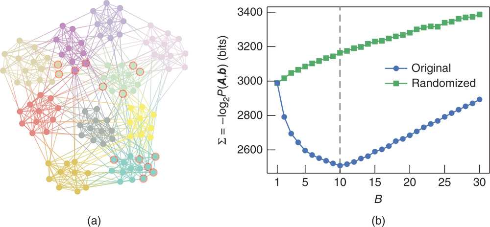
Figure 11.3 Bayesian inference of the SBM for a network of American college football teams [30]. (a) The partition that maximizes the posterior probability of Equation (11.9), or, equivalently, minimizes the description length of Equation (11.24). Nodes marked in red are not classified according to the known division into “conferences.” (b) Description length as a function of the number of groups of the corresponding optimal partition, for both the original and randomized data.
We now illustrate this approach with a real-world dataset of American college football teams [30], where a node is a team and an edge exists if two teams play against each other in a season. If we find the partition that maximizes the posterior distribution, we uncover ![]() groups, as can be seen in Figure 11.3a. If we compare this partition with the known division of the teams into “conferences” [23,24], we find that they match with a high degree of precision, with the exception of only a few nodes.12 In Figure 11.3b we show the description length of the optimal partitions if we constrain them to have a pre-specified number of groups, which allows us to see how the approach penalizes both too simple and too complex models, with a global minimum at
groups, as can be seen in Figure 11.3a. If we compare this partition with the known division of the teams into “conferences” [23,24], we find that they match with a high degree of precision, with the exception of only a few nodes.12 In Figure 11.3b we show the description length of the optimal partitions if we constrain them to have a pre-specified number of groups, which allows us to see how the approach penalizes both too simple and too complex models, with a global minimum at ![]() , corresponding to the most compressive partition. Importantly, if we now randomize the network, by placing all its edges in a completely random fashion, we obtain instead a trivial partition into
, corresponding to the most compressive partition. Importantly, if we now randomize the network, by placing all its edges in a completely random fashion, we obtain instead a trivial partition into ![]() group, indicating that the best model for this data is indeed a fully random graph. Hence, we see that this approach completely avoids the pitfall discussed in Section 11.2 and does not identify groups in fully random networks, and that the division shown in Figure 11.3a points to a statistically significant structure in the data that cannot be explained simply by random fluctuations.
group, indicating that the best model for this data is indeed a fully random graph. Hence, we see that this approach completely avoids the pitfall discussed in Section 11.2 and does not identify groups in fully random networks, and that the division shown in Figure 11.3a points to a statistically significant structure in the data that cannot be explained simply by random fluctuations.
11.6 The “Resolution Limit” Underfitting Problem and the Nested SBM
Although the Bayesian approach outlined above is in general protected against overfitting, it is still susceptible to underfitting, i.e. when we mistake statistically significant structure for randomness, resulting in the inference of an overly simplistic model. This happens whenever there is a large discrepancy between our prior assumptions and what is observed in the data. We illustrate this problem with a simple example. Consider a network formed of 64 isolated cliques of size 10, as shown in Figure 11.4a. If we employ the approach described in the previous section, and maximize the posterior of Equation (11.9), we obtain a partition into ![]() groups, where each group is composed of two cliques. This is a fairly unsatisfying characterization of this network, and also somewhat perplexing, since the probability that the inferred SBM will generate the observed network, i.e. each of the 32 groups will simultaneously and spontaneously split in two disjoint cliques, is vanishingly small. Indeed, intuitively it seems we should do significantly better with this rather obvious example, and that the best fit would be to put each of the cliques in their own group. In order to see what went wrong, we need to revisit our prior assumptions, in particular our choice for
groups, where each group is composed of two cliques. This is a fairly unsatisfying characterization of this network, and also somewhat perplexing, since the probability that the inferred SBM will generate the observed network, i.e. each of the 32 groups will simultaneously and spontaneously split in two disjoint cliques, is vanishingly small. Indeed, intuitively it seems we should do significantly better with this rather obvious example, and that the best fit would be to put each of the cliques in their own group. In order to see what went wrong, we need to revisit our prior assumptions, in particular our choice for ![]() in Equation (11.19) or, equivalently, our choice of
in Equation (11.19) or, equivalently, our choice of ![]() in Equation (11.23) for the microcanonical formulation. In both cases, they correspond to uninformative priors, which put approximately equal weight on all allowed types of large-scale structures. As argued before, this seems reasonable at first, since we should not bias our model before we observe the data. However, the implication of this choice is that we expect a priori the structure of the network at the aggregate group level, i.e. considering only the groups and the edges between them (not the individual nodes) to be fully random. This is indeed not the case in the simple example of Figure 11.4, and in fact it is unlikely to be the case for most networks that we encounter, which will probably be structured at a higher level as well. The unfavorable outcome of the uninformative assumption can also be seen by inspecting its effect on the description length of Equation (11.24). If we revisit our simple model with
in Equation (11.23) for the microcanonical formulation. In both cases, they correspond to uninformative priors, which put approximately equal weight on all allowed types of large-scale structures. As argued before, this seems reasonable at first, since we should not bias our model before we observe the data. However, the implication of this choice is that we expect a priori the structure of the network at the aggregate group level, i.e. considering only the groups and the edges between them (not the individual nodes) to be fully random. This is indeed not the case in the simple example of Figure 11.4, and in fact it is unlikely to be the case for most networks that we encounter, which will probably be structured at a higher level as well. The unfavorable outcome of the uninformative assumption can also be seen by inspecting its effect on the description length of Equation (11.24). If we revisit our simple model with ![]() cliques of size
cliques of size ![]() , grouped uniformly into
, grouped uniformly into ![]() groups of size
groups of size ![]() , and we assume that these values are sufficiently large so that Stirling's factorial approximation
, and we assume that these values are sufficiently large so that Stirling's factorial approximation ![]() can be used, the description length becomes
can be used, the description length becomes

Figure 11.4 Inference of the SBM on a simple artificial network composed of 64 cliques of size 10, illustrating the underfitting problem. (a) The partition that maximizes the posterior probability of Equation (11.9) or, equivalently, minimizes the description length of Equation (11.24). The 64 cliques are grouped into 32 groups composed of two cliques each. (b) Minimum description length as a function of the number of groups of the corresponding partition, both for the SBM and its nested variant, which is less susceptible to underfitting, and puts all 64 cliques in their own groups.
where ![]() is the total number of nodes and
is the total number of nodes and ![]() is the total number of edges, and we have omitted terms that do not depend on
is the total number of edges, and we have omitted terms that do not depend on ![]() . From this, we see that if we increase the number of groups
. From this, we see that if we increase the number of groups ![]() , this incurs a quadratic penalty in the description length given by the second term of Equation (11.27), which originates precisely from our expression of
, this incurs a quadratic penalty in the description length given by the second term of Equation (11.27), which originates precisely from our expression of ![]() : it corresponds to the amount of information necessary to describe all entries of a symmetric
: it corresponds to the amount of information necessary to describe all entries of a symmetric ![]() matrix that takes independent values between 0 and
matrix that takes independent values between 0 and ![]() . Indeed, a slightly more careful analysis of the scaling of the description length [79,85] reveals that this approach is unable to uncover a number of groups that is larger than
. Indeed, a slightly more careful analysis of the scaling of the description length [79,85] reveals that this approach is unable to uncover a number of groups that is larger than ![]() , even if their existence is obvious, as in our example of Figure 11.4.13
, even if their existence is obvious, as in our example of Figure 11.4.13
Trying to avoid this limitation might seem like a conundrum, since replacing the uninformative prior for ![]() amounts to making a more definite statement on the most likely large-scale structures that we expect to find, which we might hesitate to stipulate, as this is precisely what we want to discover from the data in the first place, and we want to remain unbiased. Luckily, there is in fact a general approach available to us to deal with this problem: we postpone our decision about the higher-order aspects of the model until we observe the data. In fact, we already saw this approach in action when we decided on the prior for the partitions; we do so by replacing the uninformative prior with a parametric distribution, whose parameters are in turn modelled by a another distribution, i.e. a hyperprior. The parameters of the prior then become latent variables that are learned from data, allowing us to uncover further structures, while remaining unbiased.
amounts to making a more definite statement on the most likely large-scale structures that we expect to find, which we might hesitate to stipulate, as this is precisely what we want to discover from the data in the first place, and we want to remain unbiased. Luckily, there is in fact a general approach available to us to deal with this problem: we postpone our decision about the higher-order aspects of the model until we observe the data. In fact, we already saw this approach in action when we decided on the prior for the partitions; we do so by replacing the uninformative prior with a parametric distribution, whose parameters are in turn modelled by a another distribution, i.e. a hyperprior. The parameters of the prior then become latent variables that are learned from data, allowing us to uncover further structures, while remaining unbiased.
The microcanonical formulation allows us to proceed in this direction in a straightforward manner, as we can interpret the matrix of edge counts ![]() as the adjacency matrix of a multigraph where each of the groups is represented as a single node. Within this interpretation, an elegant solution presents itself, where we describe the matrix
as the adjacency matrix of a multigraph where each of the groups is represented as a single node. Within this interpretation, an elegant solution presents itself, where we describe the matrix ![]() with another SBM, i.e. we partition each of the groups into meta-groups and the edges between groups are placed according to the edge counts between meta-groups. For this second SBM, we can proceed in the same manner and model it by a third SBM, and so on, forming a nested hierarchy, as illustrated in Figure 11.5 [82]. More precisely, if we denote by
with another SBM, i.e. we partition each of the groups into meta-groups and the edges between groups are placed according to the edge counts between meta-groups. For this second SBM, we can proceed in the same manner and model it by a third SBM, and so on, forming a nested hierarchy, as illustrated in Figure 11.5 [82]. More precisely, if we denote by ![]() ,
, ![]() and
and ![]() the number of groups, the partition and the matrix of edge counts at level
the number of groups, the partition and the matrix of edge counts at level ![]() , we have
, we have

with ![]() counting the number of
counting the number of ![]() -combinations with repetitions from a set of size
-combinations with repetitions from a set of size ![]() . Equation (11.28) is the likelihood of a maximum-entropy multigraph SBM, i.e. every multigraph occurs with the same probability, provided they fulfill the imposed constraints14 [78]. The prior for the partitions is again given by Equation (11.17),
. Equation (11.28) is the likelihood of a maximum-entropy multigraph SBM, i.e. every multigraph occurs with the same probability, provided they fulfill the imposed constraints14 [78]. The prior for the partitions is again given by Equation (11.17),
with ![]() , so that the joint probability of the data, edge counts, and the hierarchical partition
, so that the joint probability of the data, edge counts, and the hierarchical partition ![]() becomes
becomes

where we impose the boundary conditions ![]() and
and ![]() . We can treat the hierarchy depth
. We can treat the hierarchy depth ![]() as a latent variable as well, by placing a prior on it
as a latent variable as well, by placing a prior on it ![]() , where
, where ![]() is the maximum value allowed. But since this only contributes to an overall multiplicative constant, it has no effect on the posterior distribution, and thus can be omitted. If we impose
is the maximum value allowed. But since this only contributes to an overall multiplicative constant, it has no effect on the posterior distribution, and thus can be omitted. If we impose ![]() , we recover the uninformative prior for
, we recover the uninformative prior for ![]() ,
,

which is different from Equation (11.23) only in that the number of edges ![]() is not allowed to fluctuate.15 The inference of this model is done in the same manner as the uninformative one, by obtaining the posterior distribution of the hierarchical partition
is not allowed to fluctuate.15 The inference of this model is done in the same manner as the uninformative one, by obtaining the posterior distribution of the hierarchical partition

and the description length is given analogously by
This approach has a series of advantages; in particular, we remain a priori agnostic with respect to what kind of large-scale structure is present in the network, having constrained ourselves simply in that it can be represented as a SBM at a higher level, and with the uninformative prior as a special case. Despite this, we are able to overcome the underfitting problem encountered with the uninformative approach: if we apply this model to the example of Figure 11.4, we can successfully distinguish all 64 cliques, and provide a lower overall description length for the data, as can be seen in Figure 11.4b. More generally, by investigating the properties of the model likelihood, it is possible to show that the maximum number of groups that can be uncovered with this model scales as ![]() , which is significantly larger than the limit with uninformative priors [82,85]. The difference between both approaches manifests itself very often in practice, as shown in Figure 11.5b, where systematic underfitting is observed for a wide variety of network datasets, which disappears with the nested model, as seen in Figure 11.5c. Crucially, we achieve this decreased tendency to underfit without sacrificing our protection against overfitting: Despite the more elaborate model specification, the inference of the nested SBM is completely nonparametric, and the same Bayesian and information-theoretical principles still hold. Furthermore, as we have already mentioned, the uninformative case is a special case of the nested SBM, i.e. when
, which is significantly larger than the limit with uninformative priors [82,85]. The difference between both approaches manifests itself very often in practice, as shown in Figure 11.5b, where systematic underfitting is observed for a wide variety of network datasets, which disappears with the nested model, as seen in Figure 11.5c. Crucially, we achieve this decreased tendency to underfit without sacrificing our protection against overfitting: Despite the more elaborate model specification, the inference of the nested SBM is completely nonparametric, and the same Bayesian and information-theoretical principles still hold. Furthermore, as we have already mentioned, the uninformative case is a special case of the nested SBM, i.e. when ![]() , and hence it can only improve the inference (e.g. by reducing the description length), with no drawbacks. We stress that the number of hierarchy levels, as with any other dimension of the model, such as the number of groups in each level, is inferred from data and does not need to be determined a priori.
, and hence it can only improve the inference (e.g. by reducing the description length), with no drawbacks. We stress that the number of hierarchy levels, as with any other dimension of the model, such as the number of groups in each level, is inferred from data and does not need to be determined a priori.

Figure 11.5 (a) Diagrammatic representation of the nested SBM described in the text, with  levels, adapted from [82]. (b) Average group sizes
  obtained with the SBM using uninformative priors, for a variety of empirical networks, listed in [82]. The dashed line shows a slope
  , highlighting the systematic underfitting problem. (c) The same as in (b), but using the nested SBM, where the underfitting has virtually disappeared, with datasets randomly scattered in the allowed range.
In addition to the above, the nested model also gives us the capacity of describing the data at multiple scales, which could potentially exhibit different mixing patterns. This is particularly useful for large networks, where the SBM might still give us a very complex description, which becomes easier to interpret if we concentrate first on the upper levels of the hierarchy. A good example is the result obtained for the internet topology at the autonomous systems level, shown in Figure 11.6. The lowest level of the hierarchy shows a division into a large number of groups, with a fairly complicated structure, whereas the higher levels show an increasingly simplified picture, culminating in a core-periphery organization as the dominating pattern.

Figure 11.6 Fit of the (degree-corrected) nested SBM for the internet topology at the autonomous systems level, adapted from [82]. The hierarchical division reveals a core-periphery organization at the higher levels, where most routes go through a relatively small number of nodes (shown in the inset and in the map). The lower levels reveal a more detailed picture, where a large number of groups of nodes are identified according to their routing patterns (amounting largely to distinct geographical regions). The layout is obtained with an edge bundling algorithm by Holten [45], which uses the hierarchical partition to route the edges.
11.7 Model Variations
Varying the number of groups and building hierarchies is not the only way we have of adapting the complexity of the model to the data. We may also change the internal structure of the model, and how the division into groups affects the placement of edges. In fact, the basic ansatz of the SBM is very versatile, and many variations have been proposed in the literature. In this section we review two important ones – SBMs with degree correction and group overlap – and review other model flavors in a summarized manner.
Before we go further into the model variations, we point out that the multiplicity of models is a strength of the inference approach. This is different from the broader field of network clustering, where a large number of available algorithms often yield conflicting results for the same data, leaving practitioners lost in how to select between them [32,46]. Instead, within the inference framework we can in fact compare different models in a principled manner and select the best one according to the statistical evidence available. We proceed with a general outline of the model selection procedure before following with specific model variations.
11.7.1 Model Selection
Suppose we define two versions of the SBM, labeled ![]() and
and ![]() , each with their own posterior distribution of partitions,
, each with their own posterior distribution of partitions, ![]() and
and ![]() . Suppose we find the most likely partitions
. Suppose we find the most likely partitions ![]() and
and ![]() , according to
, according to ![]() and
and ![]() , respectively. How do we decide which partition is more representative of the data? The consistent approach is to obtain the so-called posterior odds ratio [48,49]
, respectively. How do we decide which partition is more representative of the data? The consistent approach is to obtain the so-called posterior odds ratio [48,49]

where ![]() is our prior belief that variant
is our prior belief that variant ![]() is valid. A value of
is valid. A value of ![]() indicates that the choice
indicates that the choice ![]() is
is ![]() times more plausible as an explanation for the data than the alternative,
times more plausible as an explanation for the data than the alternative, ![]() . If we are a priori agnostic with respect to which model flavor is best, i.e.
. If we are a priori agnostic with respect to which model flavor is best, i.e. ![]() , we have then
, we have then

where ![]() is the description length difference between both choices. Hence, we should generally prefer the model choice that is most compressive, i.e. with the smallest description length. However, if the value of
is the description length difference between both choices. Hence, we should generally prefer the model choice that is most compressive, i.e. with the smallest description length. However, if the value of ![]() is close to 1, we should refrain from forcefully rejecting the alternative, as the evidence in data would not be strongly decisive either way. In other words the actual value of
is close to 1, we should refrain from forcefully rejecting the alternative, as the evidence in data would not be strongly decisive either way. In other words the actual value of ![]() gives us the confidence with which we can choose the preferred model. The final decision, however, is subjective, since it depends on what we might consider plausible. A value of
gives us the confidence with which we can choose the preferred model. The final decision, however, is subjective, since it depends on what we might consider plausible. A value of ![]() , for example, typically cannot be used to forcefully reject the alternative hypothesis, whereas a value of
, for example, typically cannot be used to forcefully reject the alternative hypothesis, whereas a value of ![]() might.
might.
An alternative test we can make is to decide which model class is most representative of the data, when averaged over all possible partitions. In this case, we proceed in an analogous way by computing the posterior odds ratio

where
is the model evidence. When ![]() ,
, ![]() is called the Bayes factor, with an interpretation analogous to
is called the Bayes factor, with an interpretation analogous to ![]() above, but where the statement is made with respect to all possible partitions, not only the most likely one. Unfortunately, as mentioned previously, the evidence
above, but where the statement is made with respect to all possible partitions, not only the most likely one. Unfortunately, as mentioned previously, the evidence ![]() cannot be computed exactly for the models we are interested in, making this criterion more difficult to employ in practice (although approximations have been proposed, see e.g. [85]). We return to the issue of when it should we optimize or sample from the posterior distribution in Section 11.9, and hence which of the two criteria should be used.
cannot be computed exactly for the models we are interested in, making this criterion more difficult to employ in practice (although approximations have been proposed, see e.g. [85]). We return to the issue of when it should we optimize or sample from the posterior distribution in Section 11.9, and hence which of the two criteria should be used.
11.7.2 Degree Correction
The underlying assumption of all variants of the SBM considered so far is that nodes that belong to the same group are statistically equivalent. As it turns out, this fundamental aspect results in a very unrealistic property. Namely, this generative process implies that all nodes that belong to the same group receive on average the same number of edges. However, a common property of many empirical networks is that they have very heterogeneous degrees, often broadly distributed over several orders of magnitudes [66]. Therefore, in order for this property to be reproduced by the SBM, it is necessary to group nodes according to their degree, which may lead to some seemingly odd results. An example of this was given in [50] and is shown in Figure 11.7a. It corresponds to a fit of the SBM to a network of political blogs recorded during the 2004 American presidential election campaign [2], where an edge exists between two blogs if one links to the other. If we guide ourselves by the layout of the figure, we identify two assortative groups, which happen to be those aligned with the Republican and Democratic parties. However, inside each group there is a significant variation in degree, with a few nodes with many connections and many with very few. Because of what just has been explained, if we perform a fit of the SBM using only ![]() groups, it prefers to cluster the nodes into high-degree and low-degree groups, completely ignoring the party alliance.16 Arguably, this is a bad fit of this network, since – similarly to the underfitting example of Figure 11.4 – the probability of the fitted SBM generating a network with such a party structure is vanishingly small. In order to solve this undesired behavior, Karrer and Newman [50] proposed a modified model, which they dubbed the degree-corrected SBM (DC-SBM). In this variation, each node
groups, it prefers to cluster the nodes into high-degree and low-degree groups, completely ignoring the party alliance.16 Arguably, this is a bad fit of this network, since – similarly to the underfitting example of Figure 11.4 – the probability of the fitted SBM generating a network with such a party structure is vanishingly small. In order to solve this undesired behavior, Karrer and Newman [50] proposed a modified model, which they dubbed the degree-corrected SBM (DC-SBM). In this variation, each node ![]() is attributed with a parameter
is attributed with a parameter ![]() that controls its expected degree, independently of its group membership. Given this extra set of parameters, a network is generated with probability
that controls its expected degree, independently of its group membership. Given this extra set of parameters, a network is generated with probability

where ![]() again controls the expected number of edges between groups
again controls the expected number of edges between groups ![]() and
and ![]() . Note that since the parameters
. Note that since the parameters ![]() and
and ![]() always appear multiplying each other in the likelihood, their individual values may be arbitrarily scaled, provided their products remain the same. If we choose the parametrization
always appear multiplying each other in the likelihood, their individual values may be arbitrarily scaled, provided their products remain the same. If we choose the parametrization ![]() for every group
for every group ![]() , then they acquire a simple interpretation:
, then they acquire a simple interpretation: ![]() is the expected number of edges between groups
is the expected number of edges between groups ![]() ans
ans ![]() ,
, ![]() , and
, and ![]() is proportional to the expected degree of node
is proportional to the expected degree of node ![]() ,
, ![]() .
.
When inferring this model from the political blogs data – again forcing ![]() – we obtain a much more satisfying result, where the two political factions are neatly identified, as seen in Figure 11.7b. As this model is capable of fully decoupling the community structure from the degrees, which are captured separately by the parameters
– we obtain a much more satisfying result, where the two political factions are neatly identified, as seen in Figure 11.7b. As this model is capable of fully decoupling the community structure from the degrees, which are captured separately by the parameters ![]() and
and ![]() , respectively, the degree heterogeneity of the network does not interfere with the identification of the political factions.
, respectively, the degree heterogeneity of the network does not interfere with the identification of the political factions.
Based on the above example, and on the knowledge that most networks possess heterogeneous degrees, we could expect the DC-SBM to provide a better fit for most of them. However, before we jump to this conclusion, we must first acknowledge that the seemingly increased quality of fit obtained with the SBM came at the expense of adding an extra set of parameters, ![]() [110]. However intuitive we might judge the improvement brought on by degree correction, simply adding more parameters to a model is an almost sure recipe for overfitting. Therefore, a more prudent approach is once more to frame the inference problem in a Bayesian way, by focusing on the posterior distribution
[110]. However intuitive we might judge the improvement brought on by degree correction, simply adding more parameters to a model is an almost sure recipe for overfitting. Therefore, a more prudent approach is once more to frame the inference problem in a Bayesian way, by focusing on the posterior distribution ![]() , and on the description length. For this, we must include a prior for the node propensities
, and on the description length. For this, we must include a prior for the node propensities ![]() . The uninformative choice is the one which ascribes the same probability to all possible choices,
. The uninformative choice is the one which ascribes the same probability to all possible choices,

Figure 11.7 Inferred partition for a network of political blogs [2] using (a) the SBM and (b) the DC-SBM, in both cases forcing  groups. The node sizes are proportional to the node degrees. The SBM divides the network into low and high-degree groups, whereas the DC-SBM prefers the division into political factions.
Using again an uninformative prior for ![]() ,
,

with ![]() , the marginal likelihood now becomes
, the marginal likelihood now becomes

where ![]() is the degree of node
is the degree of node ![]() , which can be used in the same way to obtain a posterior for
, which can be used in the same way to obtain a posterior for ![]() , via Equation (11.9). Once more, the model above is equivalent to a microcanonical formulation [85], given by
, via Equation (11.9). Once more, the model above is equivalent to a microcanonical formulation [85], given by
with


and ![]() given by Equation (11.23). In the model above,
given by Equation (11.23). In the model above, ![]() is the probability of generating a multigraph where the edge counts between groups as well as the degrees
is the probability of generating a multigraph where the edge counts between groups as well as the degrees ![]() are fixed to specific values (see Figure 11.8).17 The prior
are fixed to specific values (see Figure 11.8).17 The prior ![]() is the uniform probability of generating a degree sequence, where all possibilities that satisfy the constraints imposed by the edge counts
is the uniform probability of generating a degree sequence, where all possibilities that satisfy the constraints imposed by the edge counts ![]() , namely
, namely ![]() , occur with the same probability. The description length of this model is then given by
, occur with the same probability. The description length of this model is then given by
Because uninformative priors were used to derive the above equations, we are once more subject to the same underfitting problem described previously. Luckily, from the microcanonical model we can again derive a nested DC-SBM, by replacing ![]() by a nested sequence of SBMs, exactly in the same was as was done before [82,85]. We also have the opportunity of replacing the uninformative prior for the degrees in Equation (11.44) with a more realistic option. As was argued in [85], degree sequences generated by Equation (11.44) result in exponential degree distributions, which are not quite as heterogeneous as what is often encountered in practice. A more refined approach, which is already familiar to us at this point, is to increase the Bayesian hierarchy and choose a prior that is conditioned on a higher-order aspect of the data, in this case the frequency of degrees, i.e.
by a nested sequence of SBMs, exactly in the same was as was done before [82,85]. We also have the opportunity of replacing the uninformative prior for the degrees in Equation (11.44) with a more realistic option. As was argued in [85], degree sequences generated by Equation (11.44) result in exponential degree distributions, which are not quite as heterogeneous as what is often encountered in practice. A more refined approach, which is already familiar to us at this point, is to increase the Bayesian hierarchy and choose a prior that is conditioned on a higher-order aspect of the data, in this case the frequency of degrees, i.e.
where ![]() , with
, with ![]() being the number of nodes of degree
being the number of nodes of degree ![]() in group
in group ![]() . In the above,
. In the above, ![]() is a uniform distribution of frequencies and
is a uniform distribution of frequencies and ![]() generates the degrees according to the sampled frequencies (we omit the respective expressions for brevity, and refer to [85] instead). Thus, this model is capable of using regularities in the degree distribution to inform the division into groups and is generally capable of better fits than the uniform model of Equation (11.44).
generates the degrees according to the sampled frequencies (we omit the respective expressions for brevity, and refer to [85] instead). Thus, this model is capable of using regularities in the degree distribution to inform the division into groups and is generally capable of better fits than the uniform model of Equation (11.44).

Figure 11.8 Illustration of the generative process of the microcanonical DC-SBM. Given a partition of the nodes, the edge counts between groups are sampled (a), followed by the degrees of the nodes (b) and finally the network itself (c). Adapted from [85].

Figure 11.9 Most likely hierarchical partitions of a network of political blogs [2], according to the three model variants considered, as well as the inferred number of groups  at the bottom of the hierarchy, and the description length
  : (a) NDC-SBM,
  ,
,  bits, (b) DC-SBM,
  ,
,  bits, (c) DC-SBM with the degree prior of Equation (11.46),
  ,
,  bits. The nodes circled in blue were classified as “liberals” and the remaining ones as “conservatives” in [2] based on the blog contents. Adapted from [85].
If we apply this nonparametric approach to the same political blog network of Adamic and Glance [2], we find a much more detailed picture of its structure, revealing many more than two groups, as shown in Figure 11.9, for three model variants: the nested SBM, the nested DC-SBM, and the nested DC-SBM with the degree prior of Equation (11.46). All three model variants are in fact capable of identifying the same Republican/Democrat division at the topmost hierarchical level, showing that the non-degree-corrected SBM is not as inept in capturing this aspect of the data as the result obtained by forcing ![]() might suggest. However, the internal divisions of both factions that they uncover are distinct from each other. If we inspect the obtained values of the description length with each model we see that the DC-SBM (in particular when using Equation (11.46)) results in a smaller value, indicating that it better captures the structure of the data, despite the increased number of parameters. Indeed, a systematic analysis carried out in [85] showed that the DC-SBM does in fact yield shorter description lengths for a majority of empirical datasets, thus ultimately confirming the original intuition behind the model formulation.
might suggest. However, the internal divisions of both factions that they uncover are distinct from each other. If we inspect the obtained values of the description length with each model we see that the DC-SBM (in particular when using Equation (11.46)) results in a smaller value, indicating that it better captures the structure of the data, despite the increased number of parameters. Indeed, a systematic analysis carried out in [85] showed that the DC-SBM does in fact yield shorter description lengths for a majority of empirical datasets, thus ultimately confirming the original intuition behind the model formulation.
11.7.3 Group Overlaps
Another way we can change the internal structure of the model is to allow the groups to overlap, i.e. we allow a node to belong to more than one group at the same time. The connection patterns of the nodes are then assumed to be a mixture of the “pure” groups, which results in a richer type of model [5]. Following Ball et al. [7], we can adapt the Poisson formulation to overlapping SBMs in a straightforward manner,

with
where ![]() is the probability with which node
is the probability with which node ![]() is chosen from group
is chosen from group ![]() , so that
, so that ![]() , and
, and ![]() is once more the expected number of edges between groups
is once more the expected number of edges between groups ![]() and
and ![]() . The parameters
. The parameters ![]() replace the disjoint partition
replace the disjoint partition ![]() we have been using so far by a “soft” clustering into overlapping categories.18 Note, however, that this model is a direct generalization of the non-overlapping DC-SBM of Equation (11.38), which is recovered simply by choosing
we have been using so far by a “soft” clustering into overlapping categories.18 Note, however, that this model is a direct generalization of the non-overlapping DC-SBM of Equation (11.38), which is recovered simply by choosing ![]() . The Bayesian formulation can also be performed by using an uninformative prior for
. The Bayesian formulation can also be performed by using an uninformative prior for ![]() ,
,
in addition to the same prior for ![]() in Equation (11.40). Unfortunately, computing the marginal likelihood using Equation (11.47) directly,
in Equation (11.40). Unfortunately, computing the marginal likelihood using Equation (11.47) directly,

is not tractable, which prevents us from obtaining the posterior ![]() . Instead, it is more useful to consider the auxiliary labelled matrix, or tensor,
. Instead, it is more useful to consider the auxiliary labelled matrix, or tensor, ![]() , where
, where ![]() is a particular decomposition of
is a particular decomposition of ![]() where the two edge endpoints – or “half-edges” – of an edge
where the two edge endpoints – or “half-edges” – of an edge ![]() are labelled with groups
are labelled with groups ![]() , such that
, such that
Since a sum of Poisson variables is also distributed according to a Poisson, we can write Equation (11.47) as

with each half-edge labelling being generated by

We can now compute the marginal likelihood as

which is very similar to Equation (11.41) for the DC-SBM. With the above, and knowing from Equation (11.51) that there is only one choice of ![]() that is compatible with any given
that is compatible with any given ![]() , i.e.
, i.e.

we can sample from (or maximize) the posterior distribution of the half-edge labels ![]() , just like we did for the node partition
, just like we did for the node partition ![]() in the nonoverlapping models,
in the nonoverlapping models,

where the product in the last term only accounts for choices of ![]() which are compatible with
which are compatible with ![]() , i.e. fulfill Equation (11.51). Once more, the model of Equation (11.54) is equivalent to its microcanonical analogue [84],
, i.e. fulfill Equation (11.51). Once more, the model of Equation (11.54) is equivalent to its microcanonical analogue [84],
where


and ![]() given by Equation (11.23). The variables
given by Equation (11.23). The variables ![]() are the labelled degrees of the labelled network
are the labelled degrees of the labelled network ![]() , where
, where ![]() is the number of incident edges of type
is the number of incident edges of type ![]() a node
a node ![]() has. The description length becomes likewise
has. The description length becomes likewise
The nested variant can be once more obtained by replacing ![]() in the same manner as before, and
in the same manner as before, and ![]() in a manner that is conditioned on the labelled degree frequencies and degree of overlap, as described in detail in [84].
in a manner that is conditioned on the labelled degree frequencies and degree of overlap, as described in detail in [84].
Equipped with this more general model, we may ask ourselves again if it provides a better fit of most networks, like we did for the DC-SBM in the previous section. Indeed, since the model is more general, we might conclude that this is a inevitability. However, this could be a fallacy, since more general models also include more parameters and hence are more likely to overfit. Indeed, previous claims about the existence of “pervasive overlap” in networks, based on nonstatistical methods [3], seemed to be based to some extent on this problematic logic. Claims about community overlaps are very different from, for example, the statement that networks possess heterogeneous degrees, since community overlap is not something that can be observed directly; instead it is something that must be inferred, which is precisely what our Bayesian approach is designed to do in a methodologically correct manner. An example of such a comparison is shown in Figure 11.10, for a small network of political books. This network, when analyzed using the nonoverlapping SBM, seems to be composed of three groups, easily interpreted as “left wing,” “right wing” and “center,” as the available metadata corroborates. If we fit the overlapping SBM, we observe a mixed division into the same kinds of group. If we force the inference of only two groups, we see that some of the “center” nodes are split between “right wing” or “left wing.” The latter might seem like a more pleasing interpretation, but looking at the description length reveals that it does not improve the description of the data. The best model in this case does seem to be the overlapping SBM with ![]() groups. However, the difference in the description length between all model variants is not very large, making it difficult to fully reject any of the three variants. A more systematic analysis done in [84] revealed that for most empirical networks, in particular larger ones, the overlapping models do not provide the best fits in the majority of cases, and yield larger description lengths than the nonoverlapping variants. Hence it seems that the idea of overlapping groups is less pervasive than that of degree heterogeneity, at least according to our modeling ansatz.
groups. However, the difference in the description length between all model variants is not very large, making it difficult to fully reject any of the three variants. A more systematic analysis done in [84] revealed that for most empirical networks, in particular larger ones, the overlapping models do not provide the best fits in the majority of cases, and yield larger description lengths than the nonoverlapping variants. Hence it seems that the idea of overlapping groups is less pervasive than that of degree heterogeneity, at least according to our modeling ansatz.

Figure 11.10 Network of co-purchases of books about US politics [54], with groups inferred using (a) the non-overlapping DC-SBM, with description length  bits, (b) the overlapping SBM with description length
  bits, and (c) the overlapping SBM forcing only
  groups, with description length
  bits.
bits.
It should be emphasized that we can always represent a network generated by an overlapping SBM by one generated with the nonoverlapping SBM with a larger number of groups representing the individual types of mixtures. Although model selection gives us the most parsimonious choice between the two, it does not remove the equivalence. In Figure 11.11 we show how networks generated by the overlapping SBM can be better represented by the nonoverlapping SBM (i.e. with a smaller description length) as long as the overlapping regions are sufficiently large.
11.7.4 Further Model Extensions
The simple and versatile nature of the SBM has spawned a large family of extensions and generalizations incorporating various types of more realistic features. This includes, for example, versions of the SBM that are designed for networks with continuous edge covariates (a.k.a. edge weights) [4,86], multilayer networks that are composed of different types of edges [18,74,83,101,103], networks that evolve in time [13,27,29,59,76,87,108,113], networks that possess node attributes [75] or are annotated with metadata [47,69], networks with uncertain structure [58], as well as networks that do not possess a discrete modular structure at all, and are instead embedded in generalized continuous spaces [70]. These model variations are too numerous to be described here in any detail, but it suffices to say that the general Bayesian approach outlined here, including model selection, also applicable to these variations, without any conceptual difficulty.
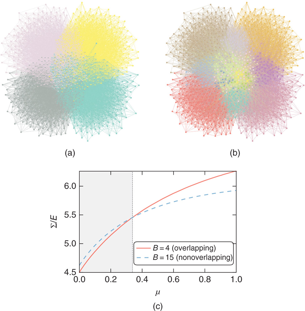
Figure 11.11 (a) Artificial network sampled from an assortative overlapping SBM with  groups and expected mixture sizes given by
  , with
  controlling the degree of overlap (see [83] for details). (b) the same network as in (a), but generated according to an equivalent nonoverlapping SBM with
  groups. (c) Description length per edge
  for the same models in (a) and (b), as a function of the degree of overlap
  , showing a cross-over where the nonoverlapping model is preferred. Adapted from [83].
11.8 Efficient Inference Using Markov Chain Monte Carlo
Although we can write exact expressions for the posterior probability of Equation (11.9) (up to a normalization constant) for a variety of model variants, the resulting distributions are not simple enough to allow us to sample from them – much less find their maximum – in a direct manner. In fact, fully characterizing the posterior distribution or finding its maximum is, for most models like the SBM, typically a NP-hard problem. What we can do, however, is to employ Markov chain Monte Carlo (MCMC) [68], which can be done efficiently, and in an asymptotically exact manner, as we now show. The central idea is to sample from ![]() by first starting from some initial configuration
by first starting from some initial configuration ![]() (in principle arbitrary) and making move proposals
(in principle arbitrary) and making move proposals ![]() with a probability
with a probability ![]() , such that, after a sufficiently long time, the equilibrium distribution is given exactly by
, such that, after a sufficiently long time, the equilibrium distribution is given exactly by ![]() . In particular, given any arbitrary move proposals
. In particular, given any arbitrary move proposals ![]() – with the only condition that they fulfill ergodicity, i.e. that they allow every state to be visited eventually – we can guarantee that the desired posterior distribution is eventually reached by employing the Metropolis–Hastings criterion [42,60], which dictates we should accept a given move proposal
– with the only condition that they fulfill ergodicity, i.e. that they allow every state to be visited eventually – we can guarantee that the desired posterior distribution is eventually reached by employing the Metropolis–Hastings criterion [42,60], which dictates we should accept a given move proposal ![]() with a probability
with a probability ![]() given by
given by
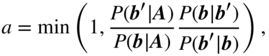
otherwise the proposal is rejected. The ratio ![]() in Equation (11.61) enforces a property known as detailed balance or reversibility, i.e.
in Equation (11.61) enforces a property known as detailed balance or reversibility, i.e.
where ![]() are the final transition probabilities after incorporating the acceptance criterion of Equation (11.61). The detailed balance condition of Equation (11.62) together with the ergodicity property guarantee that the Markov chain will converge to the desired equilibrium distribution
are the final transition probabilities after incorporating the acceptance criterion of Equation (11.61). The detailed balance condition of Equation (11.62) together with the ergodicity property guarantee that the Markov chain will converge to the desired equilibrium distribution ![]() . Importantly, we note that when computing the ratio
. Importantly, we note that when computing the ratio ![]() in Equation (11.61), we do not need to determine the intractable normalization constant of Equation (11.9), since it cancels out, and thus it can be performed exactly.
in Equation (11.61), we do not need to determine the intractable normalization constant of Equation (11.9), since it cancels out, and thus it can be performed exactly.
The above gives a generic protocol that we can use to sample from the posterior whenever we can compute the numerator of Equation (11.9). If instead we are interested in maximizing the posterior, we can introduce an “inverse temperature” parameter ![]() , by changing
, by changing ![]() in the above equations, and making
in the above equations, and making ![]() in slow increments; what is known as simulated annealing [53]. The simplest implementation of this protocol for the inference of SBMs is to start from a random partition
in slow increments; what is known as simulated annealing [53]. The simplest implementation of this protocol for the inference of SBMs is to start from a random partition ![]() , and use move proposals where a node
, and use move proposals where a node ![]() is randomly selected, and then its new group membership
is randomly selected, and then its new group membership ![]() is chosen randomly between all
is chosen randomly between all ![]() choices (where the remaining choice means we populate a new group),
choices (where the remaining choice means we populate a new group),
By inspecting Equations 11.20,11.41, (11.54) and (11.17) for all SBM variants considered, we notice that the ratio ![]() can be computed in time
can be computed in time ![]() , where
, where ![]() is the degree of node
is the degree of node ![]() , independently of other properties of the model such as the number of groups
, independently of other properties of the model such as the number of groups ![]() . Note that this is not true for all alternative formulations of the SBM, e.g. for the models in [16,33,71,90,95] computing such an update requires
. Note that this is not true for all alternative formulations of the SBM, e.g. for the models in [16,33,71,90,95] computing such an update requires ![]() time [the heat-bath move proposals of [71] increases this even further to
time [the heat-bath move proposals of [71] increases this even further to ![]() ], thus making them very inefficient for large networks, where the number of groups can reach the order of thousands or more. Hence, when using these move proposals, a full sweep of all
], thus making them very inefficient for large networks, where the number of groups can reach the order of thousands or more. Hence, when using these move proposals, a full sweep of all ![]() nodes in the network can be done in time
nodes in the network can be done in time ![]() , independent of
, independent of ![]() .
.
Although fairly simple, the above algorithm suffers from some shortcomings that can seriously degrade its performance in practice. In fact, it is typical for naive implementations of the Metropolis–Hastings algorithm to perform very badly, despite its theoretical guarantees. This is because the asymptotic properties of the Markov chain may take a very long time to be realized, and the equilibrium distribution is never observed in practical time. Generally, we should expect good convergence times only when (i) the initial state ![]() is close enough to the most likely states of the posterior and (ii) the move proposals
is close enough to the most likely states of the posterior and (ii) the move proposals ![]() resemble the shape of the posterior. Indeed, it is a trivial (and not very useful) fact that if the starting state
resemble the shape of the posterior. Indeed, it is a trivial (and not very useful) fact that if the starting state ![]() is sampled directly from the posterior, and the move proposals match the posterior exactly,
is sampled directly from the posterior, and the move proposals match the posterior exactly, ![]() , the Markov chain would be instantaneously equilibrated. Hence if we can approach this ideal scenario, we should be able to improve the inference speeds. Here we describe two simple strategies in achieving such an improvement which have been shown to yield a significance performance impact [80]. The first one is to replace the fully random move proposals of Equation (11.63) by a more informative choice. Namely, we use the current information about the model being inferred to guide our next move. We do so by selecting the membership of a node
, the Markov chain would be instantaneously equilibrated. Hence if we can approach this ideal scenario, we should be able to improve the inference speeds. Here we describe two simple strategies in achieving such an improvement which have been shown to yield a significance performance impact [80]. The first one is to replace the fully random move proposals of Equation (11.63) by a more informative choice. Namely, we use the current information about the model being inferred to guide our next move. We do so by selecting the membership of a node ![]() being moved according to
being moved according to

where ![]() is the fraction of neighbors of node
is the fraction of neighbors of node ![]() that belong to group
that belong to group ![]() , and
, and ![]() is an arbitrary parameter that enforces ergodicity, but with no other significant impact in the algorithm, provided it is sufficiently small (however, if
is an arbitrary parameter that enforces ergodicity, but with no other significant impact in the algorithm, provided it is sufficiently small (however, if ![]() we recover the fully random moves of Equation (11.63)). What this move proposal means is that we inspect the local neighborhood of the node
we recover the fully random moves of Equation (11.63)). What this move proposal means is that we inspect the local neighborhood of the node ![]() and see which groups
and see which groups ![]() are connected to this node, and we use the typical neighborhood
are connected to this node, and we use the typical neighborhood ![]() of the groups
of the groups ![]() to guide our placement of node
to guide our placement of node ![]() (see Figure 11.12a). The purpose of these move proposals is not to waste time with attempted moves that will almost surely be rejected, as will typically happen with the fully random version. We emphasize that the move proposals of Equation (11.64) do not bias the partitions toward any specific kind of mixing pattern; in particular they do not prefer assortative versus non-assortative partitions. Furthermore, these proposals can be generated efficiently, simply by following three steps: (i) sample a random neighbor
(see Figure 11.12a). The purpose of these move proposals is not to waste time with attempted moves that will almost surely be rejected, as will typically happen with the fully random version. We emphasize that the move proposals of Equation (11.64) do not bias the partitions toward any specific kind of mixing pattern; in particular they do not prefer assortative versus non-assortative partitions. Furthermore, these proposals can be generated efficiently, simply by following three steps: (i) sample a random neighbor ![]() of node
of node ![]() and inspect its group membership
and inspect its group membership ![]() , (ii) with probability
, (ii) with probability ![]() sample a fully random group
sample a fully random group ![]() (which can be a new group, and (iii) sample a group label
(which can be a new group, and (iii) sample a group label ![]() with a probability proportional to the number of edges leading to it from group
with a probability proportional to the number of edges leading to it from group ![]() ,
, ![]() . These steps can be performed in time
. These steps can be performed in time ![]() , again independently of
, again independently of ![]() , as long as a continuous book-keeping is made of the edges which are incident to each group, and therefore it does not affect the overall
, as long as a continuous book-keeping is made of the edges which are incident to each group, and therefore it does not affect the overall ![]() time complexity.
time complexity.
The second strategy is to choose a starting state that lies close to the mode of the posterior. We do so by performing a Fibonacci search [52] on the number of groups ![]() , where for each value we obtain the best partition from a larger partition with
, where for each value we obtain the best partition from a larger partition with ![]() using an agglomerative heuristic, composed of the following steps taken alternatively: (i) we attempt the moves of Equation (11.64) until no improvement to the posterior is observed and (ii) we merge groups together, achieving a smaller number of groups
using an agglomerative heuristic, composed of the following steps taken alternatively: (i) we attempt the moves of Equation (11.64) until no improvement to the posterior is observed and (ii) we merge groups together, achieving a smaller number of groups ![]() , stopping when
, stopping when ![]() . We do the last step by treating each group as a single node and using Equation (11.64) as a merge proposal, and selecting the ones that least decrease the posterior (see Figure 11.12b). As shown in [80], the overall complexity of this initialization algorithm is
. We do the last step by treating each group as a single node and using Equation (11.64) as a merge proposal, and selecting the ones that least decrease the posterior (see Figure 11.12b). As shown in [80], the overall complexity of this initialization algorithm is ![]() , and thus can be employed for very large networks.
, and thus can be employed for very large networks.
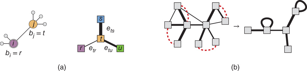
Figure 11.12 Efficient MCMC strategies. (a) Move proposals are made by inspecting the neighborhood of node  and selecting a random neighbor
  . Based on its group membership
  , the edge counts between groups are inspected (right) and the move proposal
  is made with probability proportional to
  . (b) The initial state of the MCMC is obtained with an agglomerative heuristic, where groups are merged together using the same proposals described in (a).
The approach above can be adapted to the overlapping model of Section 11.7.3, where instead of the partition ![]() , the move proposals are made with respect to the individual half-edge labels [84]. For the nested model, we have instead a hierarchical partition
, the move proposals are made with respect to the individual half-edge labels [84]. For the nested model, we have instead a hierarchical partition ![]() , and we proceed in each step of the Markov chain by randomly choosing a level
, and we proceed in each step of the Markov chain by randomly choosing a level ![]() and performing the proposals of Equation (11.64) on that level, as described in [85].
and performing the proposals of Equation (11.64) on that level, as described in [85].
The combination of the two strategies described above makes the inference procedure quite scalable, and has been successfully employed on networks on the order of ![]() to
to ![]() edges, and up to
edges, and up to ![]() groups. The MCMC algorithm described in this section, for all model variants described, is implemented in the
groups. The MCMC algorithm described in this section, for all model variants described, is implemented in the graph-tool library [81], freely available under the GPL license at http://graph-tool.skewed.de.
11.9 To Sample or To Optimize?
In the examples so far, we have focused on obtaining the most likely partition from the posterior distribution, which is the one that minimizes the description length of the data. But is this in fact the best approach? In order to answer this, we need first to quantify how well our inference is doing by comparing our estimate ![]() of the partition to the true partition that generated the data
of the partition to the true partition that generated the data ![]() , by defining a so-called loss function. For example, if we choose to be very strict, we may reject any partition that is strictly different from
, by defining a so-called loss function. For example, if we choose to be very strict, we may reject any partition that is strictly different from ![]() on equal measure, using the indicator function
on equal measure, using the indicator function
so that ![]() only if
only if ![]() , otherwise
, otherwise ![]() . If the observed data
. If the observed data ![]() and parameters
and parameters ![]() are truly sampled from the model and priors, respectively, the best assessment we can make for
are truly sampled from the model and priors, respectively, the best assessment we can make for ![]() is given by the posterior distribution
is given by the posterior distribution ![]() . Therefore, the average of the indicator over the posterior is given by
. Therefore, the average of the indicator over the posterior is given by
If we maximize ![]() with respect to
with respect to ![]() , we obtain the so-called maximum a posteriori (MAP) estimator
, we obtain the so-called maximum a posteriori (MAP) estimator
which is precisely what we have been using so far and it is equivalent to employing the MDL principle. However, using this estimator is arguably overly optimistic, as we are unlikely to find the true partition with perfect accuracy in any but the most ideal cases. Instead, we may relax our expectations and consider instead the overlap function

which measures the fraction of nodes that are correctly classified. If we maximize now the average of the overlap over the posterior distribution
we obtain the marginal estimator
where

is the marginal distribution of the group membership of node ![]() , summed over all remaining nodes.19 The marginal estimator is notably different from the MAP estimator in that it leverages information from the entire posterior distribution to inform the classification of any single node. If the posterior is tightly concentrated around its maximum, both estimators will yield compatible answers. In this situation the structure in the data is very clear, and both estimators agree. Otherwise, the estimators will yield different aspects of the data, in particular if the posterior possesses many local maxima. For example, if the data has indeed been sampled from the model we are using, the multiplicity of local maxima can be just a reflection of the randomness in the data, and the marginal estimator will be able to average over them and provide better accuracy [63,112].
, summed over all remaining nodes.19 The marginal estimator is notably different from the MAP estimator in that it leverages information from the entire posterior distribution to inform the classification of any single node. If the posterior is tightly concentrated around its maximum, both estimators will yield compatible answers. In this situation the structure in the data is very clear, and both estimators agree. Otherwise, the estimators will yield different aspects of the data, in particular if the posterior possesses many local maxima. For example, if the data has indeed been sampled from the model we are using, the multiplicity of local maxima can be just a reflection of the randomness in the data, and the marginal estimator will be able to average over them and provide better accuracy [63,112].
In view of the above, one could argue that the marginal estimator should be generally preferred over MAP. However, the situation is more complicated for data which are not sampled from model being used for inference (i.e. the model is misspecified). In this situation, multiple peaks of the distribution can point to very different partitions that are all statistically significant. These different peaks function as alternative explanations for the data that must be accepted on equal footing, according to their posterior probability. The marginal estimator will in general mix the properties of all peaks into a consensus classification that is not representative of any single hypothesis, whereas the MAP estimator will concentrate only on the most likely one (or an arbitrary choice if they are all equally likely). An illustration of this is given by the well-known Zachary's karate club network [111], which captures the social interactions between members of a karate club amidst a conflict between the club's administrator and an instructor, which lead to a split of the club in two disjoint groups. The measurement of the network was done before the final split actually happened, and it is very often used as an example of a network exhibiting community structure. If we analyze this network with the DC-SBM, we obtain three partitions that occur with very high probability from the posterior distribution: a trivial ![]() partition, corresponding to the configuration model without communities (Figure 11.13a), a “leader-follower” division into
partition, corresponding to the configuration model without communities (Figure 11.13a), a “leader-follower” division into ![]() groups, separating the administrator and instructor, together with two close allies, from the rest of the network (Figure 11.13b), and finally a
groups, separating the administrator and instructor, together with two close allies, from the rest of the network (Figure 11.13b), and finally a ![]() division into the aforementioned factions that anticipated the split (Figure 11.13c). If we would guide ourselves strictly by the MDL principle (i.e. using the MAP estimator), the preferred partition would be the trivial
division into the aforementioned factions that anticipated the split (Figure 11.13c). If we would guide ourselves strictly by the MDL principle (i.e. using the MAP estimator), the preferred partition would be the trivial ![]() one, indicating that the most likely explanation of this network is a fully random graph with a pre-specified degree sequence, and that the observed community structure emerged spontaneously. However, if we inspect the posterior distribution more closely, we see that other divisions into
one, indicating that the most likely explanation of this network is a fully random graph with a pre-specified degree sequence, and that the observed community structure emerged spontaneously. However, if we inspect the posterior distribution more closely, we see that other divisions into ![]() groups amount to around
groups amount to around ![]() of the posterior probability (see Figure 11.13e). Therefore, if we consider all
of the posterior probability (see Figure 11.13e). Therefore, if we consider all ![]() partitions collectively, they give us little reason to completely discard the possibility that the network does in fact posses some group structure. Inspecting the posterior distribution even more closely, as shown in Figure 11.13d, reveals a multimodal structure clustered around the three aforementioned partitions, giving us three very different explanations for the data, none of which can be decisively discarded in favor of the others, at least not according to the evidence available in the network structure alone.
partitions collectively, they give us little reason to completely discard the possibility that the network does in fact posses some group structure. Inspecting the posterior distribution even more closely, as shown in Figure 11.13d, reveals a multimodal structure clustered around the three aforementioned partitions, giving us three very different explanations for the data, none of which can be decisively discarded in favor of the others, at least not according to the evidence available in the network structure alone.

Figure 11.13 Posterior distribution of partitions of Zachary's karate club network using the DC-SBM. (a)–(c) show three modes of the distribution and their respective description lengths; (d) 2D projection of the posterior obtained using multidimensional scaling [15]; (e) marginal posterior distribution of the number of groups  .
.

Figure 11.14 Hierarchical partitions of a network of collaboration between scientists [67]. (a) Most likely hierarchical partition according to the DC-SBM with a uniform hyperprior. (b) Uncorrelated samples from the posterior distribution. (c) Marginal posterior distribution of the number of groups at the first three hierarchical levels, according to the model variants described in the legend. The vertical lines mark the value obtained for the most likely partition. Adapted from [85].
The situation encountered for the karate club network is a good example of the so-called bias-variance trade-off that we are often forced to face: If we choose to single-out a singe partition as a unique representation of the data, we must invariably bias our result toward any of the three most likely scenarios, discarding the remaining ones at some loss of useful information. Otherwise, if we choose to eliminate the bias by incorporating the entire posterior distribution in our representation, by the same token it will incorporate a larger variance, i.e. it will simultaneously encompass diverging explanations of the data, leaving us without an unambiguous and clear interpretation. The only situation where this trade-off is not required is when the model is a perfect fit to the data, such that the posterior is tightly peaked around a single partition. Therefore, the variance of the posterior serves as a good indication of the quality of fit of the model, providing another reason to include it in the analysis.
It should also be remarked that when using a nonparametric approach, where the dimension of the model is also inferred from the posterior distribution, the potential bias incurred when obtaining only the most likely partition usually amounts to an underfit of the data, since the uncertainty in the posterior typically translates into the existence of a more conservative partition with fewer groups.20 Instead, if we sample from the posterior distribution, we will average over many alternative fits, including those that model the data more closely with a larger number of groups. However, each individual sample of the posterior will tend to incorporate more randomness from the data, which will disappear only if we average over all samples. This means that single samples will tend to overfit the data, and hence we must resist looking at them individually. It is only in the aforementioned limit of a perfect fit that we are guaranteed not to be misled one way or another. An additional example of this is shown in Figure 11.14 for a network of collaborations among scientists. If we infer the best nested SBM, we find a specific hierarchical division of the network. However, if we sample hierarchical divisions from the posterior distribution, we typically encounter larger models, with a larger number of groups and deeper hierarchy. Each individual sample from the posterior is likely to be an overfit, but collectively they give a more accurate picture of the network in comparison with the most likely partition, which probably over-simplifies it. As already mentioned, this discrepancy, observed for all three SBM versions, tells us that neither of them is an ideal fit for this network.
The final decision on which approach to take depends on the actual objective and resources available. In general, sampling from the posterior will be more suitable when the objective is to generalize from observation and make predictions (see next section and [104]), and when computational resources are ample. Conversely, if the objective is to make a precise statement about the data, e.g. in order to summarize and interpret it, and the computational resources are scarce, maximizing the posterior tends to be more adequate.
11.10 Generalization and Prediction
When we fit a model like the SBM to a network, we are doing more than simply dividing the nodes into statistically equivalent groups; we are also making a statement about a possible mechanism that generated the network. This means that, to the extent that the model is a good representation of the data, we can use it generalize and make predictions about what has not been observed. This has been most explored for the prediction of missing and spurious links [11,37]. This represents the situation where we know or stipulate that the observed data is noisy, and may contain edges that in fact do not exist, or does not contain edges that do exist. With a generative model like the SBM, we are able to ascribe probabilities to existing and non-existing edges of being spurious or missing, respectively, as we now describe.
Following [104], the scenario we will consider is the situation where there exists a complete network ![]() which is decomposed in two parts,
which is decomposed in two parts,
where ![]() is the network that we observe, and the
is the network that we observe, and the ![]() is the set of missing and spurious edges that we want to predict, where an entry
is the set of missing and spurious edges that we want to predict, where an entry ![]() represents a missing edge and
represents a missing edge and ![]() a spurious one. Hence, our task is to obtain the posterior distribution
a spurious one. Hence, our task is to obtain the posterior distribution
The central assumption we will make is that the complete network ![]() has been generated using some arbitrary version of the SBM, with a marginal distribution
has been generated using some arbitrary version of the SBM, with a marginal distribution
Given a generated network ![]() , we then select
, we then select ![]() from some arbitrary distribution that models our source of errors
from some arbitrary distribution that models our source of errors
With the above model for the generation of the complete network and its missing and spurious edges, we can proceed to compute the posterior of Equation (11.73). We start from the joint distribution
where we have used the fact ![]() originating from Equation (11.72). For the joint distribution conditioned on the partition, we sum the above over all possible graphs
originating from Equation (11.72). For the joint distribution conditioned on the partition, we sum the above over all possible graphs ![]() , sampled from our original model,
, sampled from our original model,
The final posterior distribution of Equation (11.73) is therefore


with ![]() being a normalization constant, independent of
being a normalization constant, independent of ![]() . This expression gives a general recipe to compute the posterior, where one averages the marginal likelihood
. This expression gives a general recipe to compute the posterior, where one averages the marginal likelihood ![]() obtained by sampling partitions from the prior
obtained by sampling partitions from the prior ![]() . However, this procedure will typically take an astronomical time to converge to the correct asymptotic value, since the largest values of
. However, this procedure will typically take an astronomical time to converge to the correct asymptotic value, since the largest values of ![]() will be far away from most values of
will be far away from most values of ![]() sampled from
sampled from ![]() . A much better approach is to perform importance sampling, by rewriting the posterior as
. A much better approach is to perform importance sampling, by rewriting the posterior as


where ![]() is the posterior of partitions obtained by pretending that the observed network came directly from the SBM. We can sample from this posterior using MCMC as described in Section 11.8. As the number of entries in
is the posterior of partitions obtained by pretending that the observed network came directly from the SBM. We can sample from this posterior using MCMC as described in Section 11.8. As the number of entries in ![]() is typically much smaller than the number of observed edges, this importance sampling approach will tend to converge much faster. This allows us to compute
is typically much smaller than the number of observed edges, this importance sampling approach will tend to converge much faster. This allows us to compute ![]() in practical manner, up to a normalization constant. However, if we want to compare the relative probability between specific sets of missing/spurious edges,
in practical manner, up to a normalization constant. However, if we want to compare the relative probability between specific sets of missing/spurious edges, ![]() , via the ratio
, via the ratio

this normalization constant plays no role. The above still depends on our chosen model for the production of missing and spurious edges, given by Equation (11.75). In the absence of domain-specific information about the source of noise, we must consider all alternative choices ![]() to be equally likely a priori, so that the we can simply replace
to be equally likely a priori, so that the we can simply replace ![]() in Equation (11.83), although more realistic choices can also be included.
in Equation (11.83), although more realistic choices can also be included.
In Figure 11.15 we show the relative probabilities of two hypothetical missing edges for the American college football network, obtained with the approach above. We see that a particular missing edge between teams of the same conference is almost a hundred times more likely than one between teams of different conference.
The use of the SBM to predict missing and spurious edges has been employed in a variety of applications, such as the prediction of novel interactions between drugs [38], conflicts in social networks [94], as well to provide user recommendations [31,40], and in many cases has outperformed a variety of competing methods.
11.11 Fundamental Limits of Inference: The Detectability–Indetectability Phase Transition
Besides defining useful models and investigating their behavior in data, there is another line of questioning which deals with how far it is possible to go when we try to infer the structure of networks. Naturally, the quality of the inference depends on the statistical evidence available in the data, and we may therefore ask if it is possible at all to uncover planted structures, i.e. structures that we impose ourselves, with our inference methods, and if so, what is the best performance we can expect. Research in this area has exploded in recent years [63,112] after it was shown by Decelle et al. [19,20] that not only may it be impossible to uncover planted structures with the SBM, but the inference undergoes a “phase transition” where it becomes possible only if the structure is strong enough to cross a non-trivial threshold. This result was obtained using methods from statistical physics, which we now describe.

Figure 11.15 Two hypothetical missing edges in the network of American college football teams. The edge (a) connects teams of different conferences, whereas (b) connects teams of the same conference. According to the nested DC-SBM, their posterior probability ratios are  and
and  .
.
The situation we will consider is a “best case scenario,” where all parameters of the model are known, with the exception of the partition ![]() , this in contrast to our overall approach so far, where we considered all parameters to be unknown random variables. In particular, we will consider only the prior
, this in contrast to our overall approach so far, where we considered all parameters to be unknown random variables. In particular, we will consider only the prior
where ![]() is the probability of a node belonging in group
is the probability of a node belonging in group ![]() . Given this, we wish to obtain the posterior distribution of the node partition, using the SBM of Equation (11.8),
. Given this, we wish to obtain the posterior distribution of the node partition, using the SBM of Equation (11.8),

which was written above in terms of the “Hamiltonian”

drawing an analogy with Potts-like models in statistical physics [107]. The normalization constant, called the “partition function,” is given by
Far from being an unimportant detail, the partition function can be used to determine all statistical properties of our inference procedure. For example, if we wish to obtain the marginal posterior distribution of node ![]() , we can do so by introducing the perturbation
, we can do so by introducing the perturbation ![]() and computing the derivative
and computing the derivative

Unfortunately, it does not seem possible to compute the partition function ![]() in closed form for an arbitrary graph
in closed form for an arbitrary graph ![]() . However, there is a special case for which we can compute the partition function, namely when
. However, there is a special case for which we can compute the partition function, namely when ![]() is a tree. This is useful for us, because graphs sampled from the SBM will be “locally tree-like” if they are sparse (i.e. the degrees are small compared to the size of the network
is a tree. This is useful for us, because graphs sampled from the SBM will be “locally tree-like” if they are sparse (i.e. the degrees are small compared to the size of the network ![]() ), and the group sizes scale with the size of the system, i.e.
), and the group sizes scale with the size of the system, i.e. ![]() (which implies
(which implies ![]() ). Locally tree-like means that typical loops will have length
). Locally tree-like means that typical loops will have length ![]() , and hence at the immediate neighborhood of any given node the graph will look like a tree. Although being locally tree-like is not quite the same as being a tree, the graph will become increasing closer to being a tree in the “thermodynamic limit”
, and hence at the immediate neighborhood of any given node the graph will look like a tree. Although being locally tree-like is not quite the same as being a tree, the graph will become increasing closer to being a tree in the “thermodynamic limit” ![]() . Because of this, many properties of locally tree-like graphs will become asymptotically identical to trees in this limit. If we assume that this limit holds, we can compute the partition function by pretending that the graph is close enough to being a tree, in which case we can write the so-called Bethe free energy (we refer to [19,62] for a detailed derivation)
. Because of this, many properties of locally tree-like graphs will become asymptotically identical to trees in this limit. If we assume that this limit holds, we can compute the partition function by pretending that the graph is close enough to being a tree, in which case we can write the so-called Bethe free energy (we refer to [19,62] for a detailed derivation)

with the auxiliary quantities given by

where ![]() means the neighbors of node
means the neighbors of node ![]() . In the above equations, the values
. In the above equations, the values ![]() are called “messages” and they must fulfill the self-consistency equations
are called “messages” and they must fulfill the self-consistency equations

where ![]() means all neighbors
means all neighbors ![]() of
of ![]() excluding
excluding ![]() , the value
, the value ![]() is a normalization constant enforcing
is a normalization constant enforcing ![]() , and
, and ![]() is a local auxiliary field. Equations (11.93) are called the belief-propagation (BP) equations [62], and the entire approach is also known under the name “cavity method” [61]. The values of the messages are typically obtained by iteration, where we start from some initial configuration (e.g. a random one) and compute new values from the right-hand side of Equation (11.93), until they converge asymptotically. Note that the messages are only defined on edges of the network, and an update involves inspecting the values at the neighborhood of the nodes, where the messages can be interpreted as carrying information about the marginal distribution of a given node, if the same is removed from the network (hence the names “belief propagation” and “cavity method”). Each iteration of the BP equations can be done in time
is a local auxiliary field. Equations (11.93) are called the belief-propagation (BP) equations [62], and the entire approach is also known under the name “cavity method” [61]. The values of the messages are typically obtained by iteration, where we start from some initial configuration (e.g. a random one) and compute new values from the right-hand side of Equation (11.93), until they converge asymptotically. Note that the messages are only defined on edges of the network, and an update involves inspecting the values at the neighborhood of the nodes, where the messages can be interpreted as carrying information about the marginal distribution of a given node, if the same is removed from the network (hence the names “belief propagation” and “cavity method”). Each iteration of the BP equations can be done in time ![]() , and the convergence is often obtained only after a few iterations, rendering the whole computation fairly efficient, provided
, and the convergence is often obtained only after a few iterations, rendering the whole computation fairly efficient, provided ![]() is reasonably small. After the messages have been obtained, they can be used to compute the node marginals,
is reasonably small. After the messages have been obtained, they can be used to compute the node marginals,

where ![]() is a normalization constant.
is a normalization constant.
This whole procedure gives a way of computing the marginal distribution ![]() in a manner that is asymptotically exact, if
in a manner that is asymptotically exact, if ![]() is sufficiently large and locally tree-like. Since networks that are sampled from the SBM fulfill this property,21 we may proceed with our original question and test if we can recover the true value of
is sufficiently large and locally tree-like. Since networks that are sampled from the SBM fulfill this property,21 we may proceed with our original question and test if we can recover the true value of ![]() we used to generate a network. For the test, we use a simple parametrization named the planted partition model (PP) [12,21], where
we used to generate a network. For the test, we use a simple parametrization named the planted partition model (PP) [12,21], where ![]() and
and
with ![]() and
and ![]() specifying the expected number of edges between nodes of the same groups and of different groups, respectively. If we generate networks from this ensemble, use the BP equations to compute the posterior marginal distribution of Equation (11.94) and compare its maximum values with the planted partition, we observe, as shown in Figure 11.16, that it is recoverable only up to a certain value of
specifying the expected number of edges between nodes of the same groups and of different groups, respectively. If we generate networks from this ensemble, use the BP equations to compute the posterior marginal distribution of Equation (11.94) and compare its maximum values with the planted partition, we observe, as shown in Figure 11.16, that it is recoverable only up to a certain value of ![]() , above which the posterior distribution is fully uniform. By inspecting the stability of the fully uniform solution of the BP equations, the exact threshold can be determined [19],
, above which the posterior distribution is fully uniform. By inspecting the stability of the fully uniform solution of the BP equations, the exact threshold can be determined [19],
where ![]() is the average degree of the network. The existence of this threshold is remarkable because the ensemble is only equivalent to a completely random one if
is the average degree of the network. The existence of this threshold is remarkable because the ensemble is only equivalent to a completely random one if ![]() , yet there is a non-negligible range of values
, yet there is a non-negligible range of values ![]() for which the planted structure cannot be recovered even though the model is not random. This might seem counter-intuitive, if we argue that making
for which the planted structure cannot be recovered even though the model is not random. This might seem counter-intuitive, if we argue that making ![]() sufficiently large should at some point give us enough data to infer the model with arbitrary precision. The hole in logic lies in the fact that the number of parameters – the node partition
sufficiently large should at some point give us enough data to infer the model with arbitrary precision. The hole in logic lies in the fact that the number of parameters – the node partition ![]() – also grows with
– also grows with ![]() , and that we would need the effective sample size, i.e. the number of edges
, and that we would need the effective sample size, i.e. the number of edges ![]() , to grow faster than
, to grow faster than ![]() to guarantee that the data is sufficient. Since for sparse graphs we have
to guarantee that the data is sufficient. Since for sparse graphs we have ![]() , we are never able to reach the limit of sufficient data. Thus, we should be able to achieve asymptotically perfect inference only for dense graphs (e.g. with
, we are never able to reach the limit of sufficient data. Thus, we should be able to achieve asymptotically perfect inference only for dense graphs (e.g. with ![]() ) or by inferring simultaneously from many graphs independently sampled from the same model. Neither situation, however, is representative of what we typically encounter when we study networks.
) or by inferring simultaneously from many graphs independently sampled from the same model. Neither situation, however, is representative of what we typically encounter when we study networks.

Figure 11.16 Normalized mutual information (NMI) between the planted and inferred partitions of a PP model with  ,
,  and
and  , and
, and  . The vertical line marks the detectability threshold
  .
.
The above result carries important implications into the overall field of network clustering. The existence of the “detectable” phase for ![]() means that, in this regime, it is possible for algorithms to discover the planted partition in polynomial time, with the BP algorithm doing so optimally. Furthermore, for
means that, in this regime, it is possible for algorithms to discover the planted partition in polynomial time, with the BP algorithm doing so optimally. Furthermore, for ![]() (or
(or ![]() for the dissortative case with
for the dissortative case with ![]() ) there is another regime in a range
) there is another regime in a range ![]() , where BP converges to the planted partition only if the messages are initialized close enough to the corresponding fixed point. In this regime, the posterior landscape exhibits a “glassy” structure, with exponentially many maxima that are almost as likely as the planted partition, but are completely uncorrelated with it. The problem of finding the planted partition in this case is possible, but conjectured to be NP-hard.
, where BP converges to the planted partition only if the messages are initialized close enough to the corresponding fixed point. In this regime, the posterior landscape exhibits a “glassy” structure, with exponentially many maxima that are almost as likely as the planted partition, but are completely uncorrelated with it. The problem of finding the planted partition in this case is possible, but conjectured to be NP-hard.
Many systematic comparisons of different community detection algorithms were done in a manner that was oblivious to these fundamental facts regarding detectability and hardness [55,56], even though their existence had been conjectured before [88,92] and hence should be re-framed with it in mind. Furthermore, we point out that although the analysis based on the BP equations is mature and widely accepted in statistical physics, they are not completely rigorous from a mathematical point of view. Because of this, the result of Decelle et al. [19] leading to the threshold of Equation (11.96) has initiated intense activity from mathematicians in search of rigorous proofs, which have subsequently been found for a variety of relaxations of the original statement (see [1] for a review) and remains an active area of research.
11.12 Conclusion
In this chapter we gave a description of the basic variants of the stochastic blockmodel (SBM), and a consistent Bayesian formulation that allows us to infer them from data. The focus has been on developing a framework to extract the large-scale structure of networks while avoiding both overfitting (mistaking randomness for structure) and underfitting (mistaking structure for randomness), and doing so in a manner that is analytically tractable and computationally efficient.
The Bayesian inference approach provides a methodologically correct answer to the very central question in network analysis of whether patterns of large-scale structure can in fact be supported by statistical evidence. Besides this practical aspect, it also opens a window into the fundamental limits of network analysis itself, giving us a theoretical underpinning we can use to understand more about the nature of network systems.
Although the methods described here go a long way to allowing us to understand the structure of networks, some important open problems remain. From a modeling perspective, we know that for most systems the SBM is quite simplistic and falls very short of giving us a mechanistic explanation for them. We can interpret the SBM as being to network data what a histogram is to spatial data [73], and thus while it fulfills the formal requirements of being a generative model, it will never deplete the modeling requirements of any particular real system. Although it is naive to expect to achieve such a level of success with a general model like the SBM, it is yet still unclear how far we can go. For example, it remains to be seen how tractable it is to incorporate local structures – like densities of subgraphs – together with the large-scale structure that the SBM prescribes.
From a methodological perspective, although we can select between the various SBM flavors given the statistical evidence available, we still lack good methods to assess the quality of fit of the SBM at an absolute level. In particular, we do not yet have a systematic understanding of how well the SBM is able to reproduce properties of empirical systems, and what would be the most important sources of deficiencies, and how these could be overcome.
In addition to these outstanding challenges, there are areas of development that are more likely to undergo continuous progress. Generalizations and extensions of the SBM to cover specific cases are essentially open ended, such as the case of dynamic networks, and we can perhaps expect more realistic models to appear. Furthermore, since the inference of the SBM is in general a NP-hard problem, and thus most probably lacks a general solution, the search for more efficient algorithmic strategies that work in particular cases is also a long term goal that is likely to attract further attention.
References
- 1. E. Abbe. Community detection and stochastic block models: recent developments. arXiv:1703.10146 [cs, math, stat], Mar. 2017. arXiv: 1703.10146.
- 2. L. A. Adamic and N. Glance. The political blogosphere and the 2004 U.S. election: divided they blog. In Proceedings of the 3rd International Workshop on Link Discovery, LinkKDD '05, pages 36–43, New York, NY, USA, 2005. ACM. ISBN
- 3. Y.-Y. Ahn, J. P. Bagrow, and S. Lehmann. Link communities reveal multiscale complexity in networks. Nature, 466(7307):761–764, 2010.
- 4. C. Aicher, A. Z. Jacobs, and A. Clauset. Learning latent block structure in weighted networks. Journal of Complex Networks, 3(2):221–248, 2015.
- 5. E. M. Airoldi, D. M. Blei, S. E. Fienberg, and E. P. Xing. Mixed Membership Stochastic Blockmodels. J. Mach. Learn. Res., 9:1981–2014, 2008.
- 6. H. Akaike. A new look at the statistical model identification. IEEE Transactions on Automatic Control, 19(6):716–723, 1974.
- 7. B. Ball, B. Karrer, and M. E. J. Newman. Efficient and principled method for detecting communities in networks. Physical Review E, 84(3):036103, 2011.
- 8. G. Bianconi, P. Pin, and M. Marsili. Assessing the relevance of node features for network structure. Proceedings of the National Academy of Sciences, 106(28):11433–11438, 2009.
- 9. M. Boguñá and R. Pastor-Satorras. Class of correlated random networks with hidden variables. Physical Review E, 68(3):036112, 2003.
- 10. B. Bollobás, S. Janson, and O. Riordan. The phase transition in inhomogeneous random graphs. Random Structures & Algorithms, 31(1): 3–122, 2007.
- 11. A. Clauset, C. Moore, and M. E. J. Newman. Hierarchical structure and the prediction of missing links in networks. Nature, 453(7191):98–101, 2008.
- 12. A. Condon and R. M. Karp. Algorithms for graph partitioning on the planted partition model. Random Structures & Algorithms, 18(2): 116–140, 2001.
- 13. M. Corneli, P. Latouche, and F. Rossi. Exact ICL maximization in a non-stationary temporal extension of the stochastic block model for dynamic networks. Neurocomputing, 192:81–91, 2016.
- 14. T. M. Cover and J. A. Thomas. Elements of Information Theory. Wiley-Interscience, 99th edition, 1991.
- 15. T. F. Cox and M. A. A. Cox. Multidimensional Scaling, 2nd edition. Chapman and Hall/CRC, Boca Raton, 2000.
- 16. E. Côme and P. Latouche. Model selection and clustering in stochastic block models based on the exact integrated complete data likelihood. Statistical Modelling, 15(6):564–589, 2015.
- 17. J.-J. Daudin, F. Picard, and S. Robin. A mixture model for random graphs. Statistics and Computing, 18(2):173–183, 2008.
- 18. C. De Bacco, E. A. Power, D. B. Larremore, and C. Moore. Community detection, link prediction, and layer interdependence in multilayer networks. Physical Review E, 95(4):042317, 2017.
- 19. A. Decelle, F. Krzakala, C. Moore, and L. Zdeborová. Asymptotic analysis of the stochastic block model for modular networks and its algorithmic applications. Physical Review E, 84(6):066106, 2011.
- 20. A. Decelle, F. Krzakala, C. Moore, and L. Zdeborová. Inference and Phase Transitions in the Detection of Modules in Sparse Networks. Physical Review Letters, 107(6):065701, 2011.
- 21. M. E. Dyer and A. M. Frieze. The solution of some random NP-hard problems in polynomial expected time. Journal of Algorithms, 10(4): 451–489, 1989.
- 22. P. Erdős and A. Rényi. On random graphs, I. Publicationes Mathematicae (Debrecen), 6:290–297, 1959.
- 23. T. S. Evans. Clique graphs and overlapping communities. Journal of Statistical Mechanics: Theory and Experiment, 2010(12):P12037, 2010.
- 24. T. S. Evans. American College Football Network Files. FigShare, July 2012.
- 25. S. Fortunato. Community detection in graphs. Physics Reports, 486(3-5): 75–174, 2010.
- 26. S. Fortunato and M. Barthélemy. Resolution limit in community detection. Proceedings of the National Academy of Sciences, 104(1):36–41, 2007.
- 27. W. Fu, L. Song, and E. P. Xing. Dynamic Mixed Membership Blockmodel for Evolving Networks. In Proceedings of the 26th Annual International Conference on Machine Learning, ICML '09, pages 329–336, New York, NY, USA, 2009. ACM.
- 28. D. Garlaschelli, F. d. Hollander, and A. Roccaverde. Ensemble nonequivalence in random graphs with modular structure. Journal of Physics A: Mathematical and Theoretical, 50(1):015001, 2017.
- 29. A. Ghasemian, P. Zhang, A. Clauset, C. Moore, and L. Peel. Detectability thresholds and optimal algorithms for community structure in dynamic networks. Physical Review X, 6(3):031005, 2016.
- 30. M. Girvan and M. E. J. Newman. Community structure in social and biological networks. Proceedings of the National Academy of Sciences, 99 (12):7821–7826, June 2002.
- 31. A. Godoy-Lorite, R. Guimerà, C. Moore, and M. Sales-Pardo. Accurate and scalable social recommendation using mixed-membership stochastic block models. Proceedings of the National Academy of Sciences, 113(50): 14207–14212, 2016.
- 32. B. H. Good, Y.-A. de Montjoye, and A. Clauset. Performance of modularity maximization in practical contexts. Physical Review E, 81(4):046106, 2010.
- 33. P. K. Gopalan and D. M. Blei. Efficient discovery of overlapping communities in massive networks. Proceedings of the National Academy of Sciences, 110(36):14534–14539, 2013.
- 34. P. Grünwald. A tutorial introduction to the minimum description length principle. arXiv:math/0406077, June 2004.
- 35. P. D. Grünwald. The Minimum Description Length Principle. The MIT Press, 2007.
- 36. R. Guimerà and L. A. Nunes Amaral. Functional cartography of complex metabolic networks. Nature, 433(7028):895–900, 2005.
- 37. R. Guimerà and M. Sales-Pardo. Missing and spurious interactions and the reconstruction of complex networks. Proceedings of the National Academy of Sciences, 106(52):22073–22078, 2009.
- 38. R. Guimerà and M. Sales-Pardo. A network inference method for large-scale unsupervised identification of novel drug-drug interactions. PLoS Comput Biol, 9(12):e1003374, 2013.
- 39. R. Guimerà, M. Sales-Pardo, and L. A. N. Amaral. Modularity from fluctuations in random graphs and complex networks. Physical Review E, 70(2):025101, 2004.
- 40. R. Guimerà, A. Llorente, E. Moro, and M. Sales-Pardo. Predicting human preferences using the block structure of complex social networks. PLoS One, 7(9):e44620, 2012.
- 41. M. B. Hastings. Community detection as an inference problem. Physical Review E, 74(3):035102, 2006.
- 42. W. K. Hastings. Monte Carlo sampling methods using Markov chains and their applications. Biometrika, 57(1):97–109, 1970.
- 43. J. M. Hofman and C. H. Wiggins. Bayesian approach to network modularity. Physical Review Letters, 100(25):258701, 2008.
- 44. P. W. Holland, K. B. Laskey, and S. Leinhardt. Stochastic blockmodels: First steps. Social Networks, 5(2):109–137, 1983.
- 45. D. Holten. Hierarchical edge bundles: visualization of adjacency relations in hierarchical data. IEEE Transactions on Visualization and Computer Graphics, 12(5):741–748, 2006.
- 46. D. Hric, R. K. Darst, and S. Fortunato. Community detection in networks: Structural communities versus ground truth. Physical Review E, 90(6): 062805, 2014.
- 47. D. Hric, T. P. Peixoto, and S. Fortunato. Network structure, metadata, and the prediction of missing nodes and annotations. Physical Review X, 6(3): 031038, Sept. 2016.
- 48. E. T. Jaynes. Probability Theory: The Logic of Science. Cambridge University Press, Cambridge, New York, 2003.
- 49. H. Jeffreys. Theory of Probability. Oxford University Press, Oxford, New York, 3rd edition, 2000.
- 50. B. Karrer and M. E. J. Newman. Stochastic blockmodels and community structure in networks. Physical Review E, 83(1):016107, 2011.
- 51. C. Kemp and J. B. Tenenbaum. Learning systems of concepts with an infinite relational model. In Proceedings of the 21st National Conference on Artificial Intelligence, 2006.
- 52. J. Kiefer. Sequential Minimax Search for a Maximum. Proceedings of the American Mathematical Society, 4(3):502, 1953.
- 53. S. Kirkpatrick, C. D. Gelatt Jr, and M. P. Vecchi. Optimization by simulated annealing. Science, 220(4598):671, 1983.
- 54. V. Krebs. Analyzing one network to reveal another. Bulletin of Sociological Methodology/Bulletin de Méthodologie Sociologique, 79(1):61–70, 2003.
- 55. A. Lancichinetti and S. Fortunato. Benchmarks for testing community detection algorithms on directed and weighted graphs with overlapping communities. Physical Review E, 80(1):016118, 2009.
- 56. A. Lancichinetti, S. Fortunato, and F. Radicchi. Benchmark graphs for testing community detection algorithms. Physical Review E, 78(4):046110, 2008.
- 57. D. J. C. MacKay. Information Theory, Inference and Learning Algorithms. Cambridge University Press, 2003.
- 58. T. Martin, B. Ball, and M. E. J. Newman. Structural inference for uncertain networks. Physical Review E, 93(1):012306, 2016.
- 59. Matias Catherine and Miele Vincent. Statistical clustering of temporal networks through a dynamic stochastic block model. Journal of the Royal Statistical Society: Series B (Statistical Methodology), 79(4):1119–1141, 2016.
- 60. N. Metropolis, A. W. Rosenbluth, M. N. Rosenbluth, A. H. Teller, and E. Teller. Equation of state calculations by fast computing machines. Journal of Chemical Physics, 21(6):1087, 1953.
- 61. M. Mezard. Spin Glass Theory And Beyond: An Introduction To The Replica Method And Its Applications. WSPC, Singapore, New Jersey, 1986.
- 62. M. Mezard and A. Montanari. Information, Physics, and Computation. Oxford University Press, 2009.
- 63. C. Moore. The Computer Science and Physics of Community Detection: Landscapes, Phase Transitions, and Hardness. Feb. 2017. arXiv: 1702.00467.
- 64. M. Mørup and M. N. Schmidt. Bayesian community detection. Neural Computation, 24(9):2434–2456, 2012.
- 65. M. Mørup, M. N. Schmidt, and L. K. Hansen. Infinite multiple membership relational modeling for complex networks. In 2011 IEEE International Workshop on Machine Learning for Signal Processing, pages 1–6, 2011.
- 66. M. Newman. Networks: An Introduction. Oxford University Press, 2010.
- 67. M. E. J. Newman. Finding community structure in networks using the eigenvectors of matrices. Physical Review E, 74(3):036104, 2006.
- 68. M. E. J. Newman and G. T. Barkema. Monte Carlo Methods in Statistical Physics. Oxford University Press, oxford, New York, 1999.
- 69. M. E. J. Newman and A. Clauset. Structure and inference in annotated networks. Nature Communications, 7:11863, June 2016.
- 70. M. E. J. Newman and T. P. Peixoto. Generalized communities in networks. Physical Review Letters, 115(8):088701, 2015.
- 71. M. E. J. Newman and G. Reinert. Estimating the number of communities in a network. Physical Review Letters, 117(7):078301, 2016.
- 72. K. Nowicki and T. A. B. Snijders. Estimation and prediction for stochastic blockstructures. Journal of the American Statistical Association, 96(455): 1077–1087, 2001.
- 73. S. C. Olhede and P. J. Wolfe. Network histograms and universality of blockmodel approximation. Proceedings of the National Academy of Sciences, 111(41):14722–14727, 2014.
- 74. S. Paul and Y. Chen. Consistent community detection in multi-relational data through restricted multi-layer stochastic blockmodel. Electronic Journal of Statistics, 10(2):3807–3870, 2016.
- 75. L. Peel. Active discovery of network roles for predicting the classes of network nodes. Journal of Complex Networks, 3(3):431–449, 2015.
- 76. L. Peel and A. Clauset. Detecting change points in the large-scale structure of evolving networks. In Twenty-Ninth AAAI Conference on Artificial Intelligence, Feb. 2015.
- 77. L. Peel, D. B. Larremore, and A. Clauset. The ground truth about metadata and community detection in networks. Science Advances, 3(5): e1602548, 2017.
- 78. T. P. Peixoto. Entropy of stochastic blockmodel ensembles. Physical Review E, 85(5):056122, 2012.
- 79. T. P. Peixoto. Parsimonious module inference in large networks. Physical Review Letters, 110(14):148701, 2013.
- 80. T. P. Peixoto. Efficient Monte Carlo and greedy heuristic for the inference of stochastic block models. Physical Review E, 89(1):012804, 2014.
- 81. T. P. Peixoto. The
graph-toolpython library. figshare, 2014. Available at https://figshare.com/articles/graph_tool/1164194. - 82. T. P. Peixoto. Hierarchical block structures and high-resolution model selection in large networks. Physical Review X, 4(1):011047, 2014.
- 83. T. P. Peixoto. Inferring the mesoscale structure of layered, edge-valued, and time-varying networks. Physical Review E, 92(4):042807, 2015.
- 84. T. P. Peixoto. Model selection and hypothesis testing for large-scale network models with overlapping groups. Physical Review X, 5(1):011033, 2015.
- 85. T. P. Peixoto. Nonparametric Bayesian inference of the microcanonical stochastic block model. Physical Review E, 95(1):012317, 2017.
- 86. T. P. Peixoto. Nonparametric weighted stochastic block models. Physical Review E, 97(1):012306, 2018.
- 87. T. P. Peixoto and M. Rosvall. Modelling sequences and temporal networks with dynamic community structures. Nature Communications, 8(1):582, 2017.
- 88. J. Reichardt and M. Leone. (Un)detectable cluster structure in sparse networks. Physical Review Letters, 101(7):078701, 2008.
- 89. J. Reichardt, R. Alamino, and D. Saad. The interplay between microscopic and mesoscopic structures in complex networks. PLoS One, 6(8):e21282, 2011.
- 90. M. A. Riolo, G. T. Cantwell, G. Reinert, and M. E. J. Newman. Efficient method for estimating the number of communities in a network. Physical Review E, 96(3):032310, 2017.
- 91. J. Rissanen. Modeling by shortest data description. Automatica, 14(5): 465–471, 1978.
- 92. P. Ronhovde and Z. Nussinov. Multiresolution community detection for megascale networks by information-based replica correlations. Physical Review E, 80(1):016109, 2009.
- 93. M. Rosvall and C. T. Bergstrom. An information-theoretic framework for resolving community structure in complex networks. Proceedings of the National Academy of Sciences, 104(18):7327–7331, 2007.
- 94. N. Rovira-Asenjo, T. Gumí, M. Sales-Pardo, and R. Guimerà. Predicting future conflict between team-members with parameter-free models of social networks. Scientific Reports, 3, 2013.
- 95. M. Schmidt and M. Morup. Nonparametric Bayesian modeling of complex networks: An introduction. IEEE Signal Processing Magazine, 30(3): 110–128, 2013.
- 96. G. Schwarz. Estimating the dimension of a model. Annals of Statistics, 6 (2):461–464, 1978.
- 97. Y. M. Shtar'kov. Universal sequential coding of single messages. Problemy Peredachi Informatsii, 23(3):3–17, 1987.
- 98. N. J. A. Sloane. The on-line encyclopedia of integer sequences: A008277. 2003.
- 99. N. J. A. Sloane. The on-line encyclopedia of integer sequences: A000670. 2003.
- 100. T. A. B. Snijders and K. Nowicki. Estimation and prediction for stochastic blockmodels for graphs with latent block structure. Journal of Classification, 14(1):75–100, 1997.
- 101. N. Stanley, S. Shai, D. Taylor, and P. J. Mucha. Clustering network layers with the strata multilayer stochastic block model. IEEE Transactions on Network Science and Engineering, 3(2):95–105, 2016.
- 102. B. Söderberg. General formalism for inhomogeneous random graphs. Physical Review E, 66(6):066121, 2002.
- 103. T. Vallès-Català, F. A. Massucci, R. Guimerà, and M. Sales-Pardo. stochastic block models reveal the multilayer structure of complex networks. Physical Review X, 6(1):011036, 2016.
- 104. T. Vallès-Català, T. P. Peixoto, R. Guimerà, and M. Sales-Pardo. On the consistency between model selection and link prediction in networks. May 2017. arXiv: 1705.07967.
- 105. Y. J. Wang and G. Y. Wong. Stochastic blockmodels for directed graphs. Journal of the American Statistical Association, 82(397):8–19, 1987.
- 106. Y. X. R. Wang and P. J. Bickel. Likelihood-based model selection for stochastic block models. Annals of Statistics, 45(2):500–528, 2017.
- 107. F. Y. Wu. The Potts model. Reviews of Modern Physics, 54(1):235–268, 1982.
- 108. K. Xu and A. Hero. Dynamic stochastic blockmodels for time-evolving social networks. IEEE Journal of Selected Topics in Signal Processing, 8 (4):552–562, 2014.
- 109. X. Yan. Bayesian model selection of stochastic block models. 2016. arXiv: 1605.07057.
- 110. X. Yan, C. Shalizi, J. E. Jensen, F. Krzakala, C. Moore, L. Zdeborová, P. Zhang, and Y. Zhu. Model selection for degree-corrected block models. Journal of Statistical Mechanics: Theory and Experiment, 2014(5): P05007, 2014.
- 111. W. W. Zachary. An information flow model for conflict and fission in small groups. Journal of Anthropological Research, 33(4):452–473, 1977.
- 112. L. Zdeborová and F. Krzakala. Statistical physics of inference: thresholds and algorithms. Advances in Physics, 65(5):453–552, 2016.
- 113. X. Zhang, C. Moore, and M. E. J. Newman. Random graph models for dynamic networks. European Physical Journal B, 90(10):200, 2017.
Notes
- 1 Although the Poisson model is not strictly a maximum entropy ensemble, the generative process behind it is easy to justify. We can imagine it as the random placement of exactly
 edges into the
  entries of the matrix
  , each with a probability
  of attracting an edge, with
  , yielding a multinomial distribution
  , where, differently from Equation (11.8), the edge placements are not conditionally independent. But if we now sample the total number of edges
  from a Poisson distribution
  with average
  , by exploiting the relationship between the multinomial and Poisson distributions, we have
  , where
  , which does amount to conditionally independent edge placements. Making
  , and allowing self-loops, we arrive at Equation (11.8).
 - 2 One could argue that most networks change in time, and hence belong to a time series, thus possibly allowing priors to be selected from earlier observations of the same network. This is a potentially useful way to proceed, but also opens a Pandora's box of dynamical network models, where simplistic notions of statistical stationarity are likely to be contradicted by data. Some recent progress has been made on the inference of dynamic networks [13,27,29,59,76,87,108,113], but this field is still in relative infancy.
- 3 The name “uninformative” is something of a misnomer, as it is not really possible for priors to truly carry “no information” to the posterior distribution. In our context, the term is used simply to refer to maximum entropy priors, conditioned on specific constraints.
- 4 Using constant priors such as Equation (11.12) makes the posterior distribution proportional to the likelihood. Maximizing such a posterior distribution is therefore entirely equivalent to a “non-Bayesian” maximum likelihood approach, and nullifies our attempt to prevent overfitting.
- 5 We could have used simply
 , since
  is the number of partitions of
  nodes into
  groups, which are allowed to be empty. However, this would force us to distinguish between the nominal and the actual number of groups (discounting empty ones) during inference [71], which becomes unnecessary if we simply forbid empty groups in our prior.
 - 6 More strictly, we should treat
 just as another hyperparameter and integrate over its own distribution. But since this is just a global parameter, not affected by the dimension of the model, we can get away with setting its value directly from the data. It means we are pretending we know precisely the density of the network we are observing, which is not a very strong assumption. Nevertheless, readers who are uneasy with this procedure can rest assured that this can be completely amended once we move to microcanonical models in Section 11.6 (see footnote 15).
 - 7 Some readers may wonder why Equation (11.21) should not contain a sum, i.e.
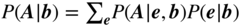 . Indeed, that is the proper way to write a marginal likelihood. However, for the microcanonical model there is only one element of the sum that fulfills the constraint of Equation (11.1), and thus yields a nonzero probability, making the marginal likelihood identical to the joint, as expressed in Equation (11.21). The same is true for the partition prior of Equation (11.17). We will use this fact in our notation throughout, and omit sums when they are unnecessary.
 - 8 This equivalence occurs for a variety of Bayesian models. For instance, if we flip a coin with a probability
 of coming up heads, the integrated likelihood under a uniform prior after
  trials in which
  heads were observed is
  . This is the same as the “microcanonical” model
 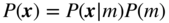 with
with  and
and  , i.e. the number of heads is sampled from a uniform distribution, and the coin flips are sampled randomly among those that have that exact number of heads.
 - 9 Sometimes the minimum description length principle (MDL) is considered as an alternative method to Bayesian inference. Although it is possible to apply the MDL in a manner that makes the connection with Bayesian inference difficult, as, for example, with the normalized maximum likelihood scheme [34,97], in its more direct and tractable form it is fully equivalent to the Bayesian approach [35]. Note also that we do not in fact require the connection with microcanonical models made here, as the description length can be defined directly as
 , without referring explicitly to internal model parameters.
 - 10 Some readers may notice the similarity between Equation (11.26) and other penalty-based criteria, such as the Bayesian information criterion (BIC) [96] and the Akaike information criterion (AIC) [6]. Although all these criteria share the same overall interpretation, BIC and AIC rely on specific assumptions about the asymptotic shape of the model likelihood, which are known to be invalid for the SBM [110], unlike Equation (11.26) which is exact.
- 11 An important result in information theory states that compressing random data is asymptotically impossible [14]. This lies at the heart of the effectiveness of the MDL approach in preventing overfitting, as incorporating randomness into the model description cannot be used to reduce the description length.
- 12 Care should be taken when comparing with “known” divisions in this manner, as there is no guarantee that the available metadata is in fact relevant for the network structure. See [47,69,77] for more detailed discussions.
- 13 This same problem occurs for slight variations of the SBM and corresponding priors, provided they are uninformative, such as those in [16,71,95], and also with other penalty-based approaches that rely on a functional form similar to Equation (11.27) [106]. Furthermore, this limitation is conspicuously similar to the “resolution limit” present in the popular heuristic of modularity maximization [26], although it is not yet clear if a deeper connection exists between both phenomena.
- 14 Note that we cannot use in the upper levels exactly the same model we use in the bottom level, given by Equation (11.22), as most terms in the subsequent levels will cancel out. This happens because the model in Equation (11.22) is based on the uniform generation of configurations, not multigraphs [85]. However, we are free to use Equation (11.28) in the bottom level as well.
- 15 The prior of Equation (11.31) and the hierarchy in Equation (11.30) are conditioned on the total number of edges
 , which is typically unknown before we observe the data. Similarly to the parameter
  in the canonical model formulation, the strictly correct approach would be to consider this quantity as an additional model parameter, with its prior distribution
  . However, in the microcanonical model there is no integration involved, and
  – regardless of how we specify it – would contribute to an overall multiplicative constant that disappears from the posterior distribution after normalization. Therefore we can simply omit it.
 - 16 It is possible that unexpected results of this kind inhibited the initial adoption of SBM methods in the network science community, which focused instead on more heuristic community detection methods, save for a few exceptions (e.g. [11,36,37,41,43,93]).
- 17 The ensemble equivalence of Equation (11.42) is in some ways more remarkable than for the traditional SBM. This is because a direct equivalence between the ensembles of Equations (11.38) and (11.43) is not satisfied even in the asymptotic limit of large networks [28,78], which does happen for Equations (11.8) and (11.22). Equivalence is observed only if the individual degrees
 also become asymptotically large. However, when the parameters
  and
and  are integrated out, the equivalence becomes exact for networks of any size.
 - 18 Note that, differently from the non-overlapping case, here it is possible for a node not to belong to any group, in which case it will never receive an incident edge.
- 19 The careful reader will notice that we must have in fact a trivial constant marginal
 for every node
  , since there is a symmetry of the posterior distribution with respect to re-labelling of the groups, in principle rendering this estimator useless. In practice, however, our samples from the posterior distribution (e.g. using MCMC) will not span the whole space of label permutations in any reasonable amount of time, and instead will concentrate on a mode around one of the possible permutations. Since the modes around the label permutations are entirely symmetric, the node marginals obtained in this manner can be meaningfully used. However, for networks where some of the groups are not very large, local permutations of individual group labels are statistically possible during MCMC inference, leading to degeneracies in the marginal
  of the affected nodes, resulting in artefacts when using the marginal estimator. This problem is exacerbated when the number of groups changes during MCMC sampling.
 - 20 This is different from parametric posteriors, where the dimension of the model is externally imposed in the prior and the MAP estimator tends to overfit [63,112].
- 21 Real networks, however, should not be expected to be locally tree-like. This does not invalidate the results of this section, which pertain strictly to data sampled from the SBM. However, despite not being exact, the BP algorithm yields surprisingly accurate results for real networks, even when the tree-like property is violated [19].