
CHAPTER 12
SIGNAL PROCESSING FOR MIMO-BASED CHIPLESS RFID SYSTEMS
12.1 INTRODUCTION
In Chapter 8, several chipless tags have been studied and it is concluded that multiresonator-based chipless tags will be further investigated in order to incorporate them with the proposed MIMO-based chipless RFID system. The main reason is that the multiresonator tags are reported as one of the chipless tag types with the largest data capacity. Also, Monash Microwave, Antennas, RFID and Sensors Laboratory (MMARS) has all the required equipment and facilities for tag fabrication and testing.
An overview of the proposed MIMO-based chipless RFID system is illustrated in Figure 12.1. The chipless tag used in the proposed system is multiresonator based, where each resonator acts as a bandstop filter introducing a frequency signature to the tag.

Figure 12.1 MIMO-based chipless RFID system.
The tag considered earlier has one receiving antenna (Rx) and two transmitting antennas (![]() and
and ![]() ) cross-polarized with Rx as shown in Figure 12.1. The RFID reader has one transmitting antenna (Tx) that is cross-polarized with its two receiving antennas (
) cross-polarized with Rx as shown in Figure 12.1. The RFID reader has one transmitting antenna (Tx) that is cross-polarized with its two receiving antennas (![]() and
and ![]() ), hence minimizing the coupling between transmitting and receiving antennas. The transmitting antenna of the reader (Tx) and the receiving antenna of the tag (Rx) are copolarized that are already cross-polarized with the transmitting antennas of the tags (
), hence minimizing the coupling between transmitting and receiving antennas. The transmitting antenna of the reader (Tx) and the receiving antenna of the tag (Rx) are copolarized that are already cross-polarized with the transmitting antennas of the tags (![]() and
and ![]() ) so that, the undesired coupling throughout the system is minimized. As a result, when the reader transmits, it is safe to assume that only Rx of the tag receives the signal, hence forming a single input single output (SISO) channel from the reader to the tag named as the forward channel hereafter.
) so that, the undesired coupling throughout the system is minimized. As a result, when the reader transmits, it is safe to assume that only Rx of the tag receives the signal, hence forming a single input single output (SISO) channel from the reader to the tag named as the forward channel hereafter.
Then the received signal at the tag will be divided into two parts using an equal power divider. Each RF component will then travel toward its transmitting antenna surrounding the frequency resonators as shown in 12.2. When an RF signal travels surrounding the resonators, the resonators start to resonate at their resonating frequency, hence losing the power in the corresponding frequency of the signal. Once the RF signal reaches the end of the transmission line, it contains the frequency signature of the tag and this process is called tag modulation hereafter. The tag-modulated RF signals will then be transmitted back to the reader by using each transmitting antenna of the tag. There will be two different signals transmitting from the tag toward the reader and the reader will receive them using two receiving antennas (![]() and
and ![]() ) having the same polarization to that of the transmitting antennas of the tag. This forms a 2×2 multiple input multiple output (MIMO) channel and is called reverse channel hereafter.
) having the same polarization to that of the transmitting antennas of the tag. This forms a 2×2 multiple input multiple output (MIMO) channel and is called reverse channel hereafter.

Figure 12.2 MIMO tag.
Tag detection involves two stages. First stage is about MIMO decomposing. When the RFID reader receives two streams of signals from its two receiving antennas, those signals are already mixed with the ![]() MIMO channel. First MIMO decoding techniques are used to decompose these already mixed two signal streams. Once they are separated, in second stage, ML-based tag detection techniques are used to identify encoded tag data.
MIMO channel. First MIMO decoding techniques are used to decompose these already mixed two signal streams. Once they are separated, in second stage, ML-based tag detection techniques are used to identify encoded tag data.
The resonator combination used in each branch of the MIMO tag can perform tag modulation individually. As a result, the bit capacity can be improved by several factors if the tag contains multiple branches. For example, a MIMO tag with two branches can double the tag bit capacity using the same frequency band of the SISO tag. This becomes achievable, thanks to the MIMO decomposing algorithms, which will be discussed in the following section.
12.2 MIMO DECOMPOSING TECHNIQUES
The signal model used in the proposed MIMO-based chipless RFID system is shown in Figure 12.3 and explained in this section.

Figure 12.3 MIMO tag operation overview.
If the interrogating signal is denoted by ![]() and the forward channel by
and the forward channel by ![]() , then the received signal at the tag
, then the received signal at the tag ![]() can be represented using (12.1), whereas
can be represented using (12.1), whereas ![]() is the noise added by the receiving antenna at the tag.
is the noise added by the receiving antenna at the tag.
Then the received noisy signal is divided into two power-equal components ![]() and
and ![]() .
.
These two identical signals are tag modulated using independently selected resonator combination. Assume that the equivalent bandstop filters of the resonator combinations in each branch are given by ![]() and
and ![]() . Then the final tag response in each branch (
. Then the final tag response in each branch (![]() and
and ![]() ) can be calculated as (12.2).
) can be calculated as (12.2).

When the tags are located closer to the reader, the signal power is considerably higher than the noise added by the receiving antenna of the tag. Therefore, noise can be neglected and the above-mentioned expressions further simplify to (12.3). ![]() and
and ![]() are the resultant signals after tag modulation in branches 1 and 2, respectively, which are independent of the forward channel.
are the resultant signals after tag modulation in branches 1 and 2, respectively, which are independent of the forward channel.

If the tag responses in (12.3) has ![]() number of samples, then these two responses can be stacked to form a matrix
number of samples, then these two responses can be stacked to form a matrix ![]() as shown (12.4).
as shown (12.4).

The received signals (![]() and
and ![]() ) at the reader antenna array can be represented using a matrix as follows:
) at the reader antenna array can be represented using a matrix as follows:
If the reverse channel is given by ![]() , the received signal array at the RFID reader can be calculated using (12.5).
, the received signal array at the RFID reader can be calculated using (12.5). ![]() is the product of the forward and the reverse channels weighted by a factor of
is the product of the forward and the reverse channels weighted by a factor of ![]() , and the noise matrix added by the both receiving antennas of the reader is given by
, and the noise matrix added by the both receiving antennas of the reader is given by ![]() .
.

Assuming the channel, ![]() is known to the RFID reader, the estimated tag responses can be calculated using standard MIMO decomposing methods. In this section, two methods are presented, namely, zero forcing (ZF) equalizer and the minimum mean square error equalizer (MMSE) as presented in (12.6).
is known to the RFID reader, the estimated tag responses can be calculated using standard MIMO decomposing methods. In this section, two methods are presented, namely, zero forcing (ZF) equalizer and the minimum mean square error equalizer (MMSE) as presented in (12.6).

![]() is the Hermitian transpose of the channel matrix
is the Hermitian transpose of the channel matrix ![]() and
and ![]() is the noise power available at the reader, which is calculated using SNR.
is the noise power available at the reader, which is calculated using SNR.
The ML-based tag detection technique derived in Section 12.4 assumes a Gaussian distribution for noise available at the reader. We have used MMSE equalizer as the decomposing technique in prior work [1]. The results are shown in Section 12.6.1 under method 1. Even though it leads to better signal to interference plus noise ratio (SINR) performance, in the process it makes noise distribution to be bimodal, hence it no longer can be treated as Gaussian. On the other hand, the noise produced after ZF method still follows a Gaussian distribution subjected to an amplified noise. Modeling the bimodal noise distribution to derive a likelihood-based detector makes the signal processing extremely complex. Therefore, only the ZF equalizer is used with the likelihood detector and the results show that even under this scenario the ML detection technique performs better than the performance reported in Ref. [1]. This method is named as method 2 and the results are presented in Section 12.6.2.
After applying the ZF equalizer, an estimated tag response for each branch can be obtained as shown in (12.7). ![]() represents the estimated tag responses in each branch.
represents the estimated tag responses in each branch.
The estimated tag response in (12.7) is derived for time-domain-based signal samples. However, the above relationship will still be applicable if a unitary transformation such as Fourier transform is performed. As a result, the estimated tag responses in frequency domain can be calculated as follows:
An ML-based tag detection technique is derived, which is later applied on these estimated tag responses. Derivation of the tag detection technique is discussed in the following section.
12.3 TAG DETECTION IN MIMO
In this section, we derive an expression for the maximum likelihood (ML) function, to detect which resonator combination (notch filters) the signal has gone through. ZF equalizer derived in the previous section produces an estimated tag response for each branch in the MIMO tag. However, it could also amplify the noise during the decomposing. As a result, the output of the ZF equalizer can be expected to be noisy. The task is to find which resonator combination has the highest maximum likelihood, out of all the possibilities. For example, if each branch had ![]() resonators, then there would be
resonators, then there would be ![]() unique tag responses in each branch. Therefore, each estimated tag response should be compared with
unique tag responses in each branch. Therefore, each estimated tag response should be compared with ![]() tag responses and the one with the highest likelihood is selected.
tag responses and the one with the highest likelihood is selected.
The signal model used is explained in what follows. If ![]() is the
is the ![]() th tag response vector out of all the
th tag response vector out of all the ![]() number of combinations and
number of combinations and ![]() is the noise vector available after ZF equalizer, then the estimated tag response vector,
is the noise vector available after ZF equalizer, then the estimated tag response vector, ![]() is given by
is given by
Due to I & Q demodulation, these signals are complex and they can be represented using real and imaginary components (![]() and
and ![]() ) as follows:
) as follows:

Therefore, the received signal can be written as

Each noise sample in ![]() is assumed to have an independent and identical distribution (i.i.d.) with zero mean and a variance of
is assumed to have an independent and identical distribution (i.i.d.) with zero mean and a variance of ![]() . Original noise added at the reader is assumed to be Gaussian due to the reader architecture. As pointed out in the previous section, ZF equalizer may only amplify the noise. As a result, the noise after the equalizer can still be treated as Gaussian. Therefore, it was assumed both the real and imaginary parts of each noise sample (
. Original noise added at the reader is assumed to be Gaussian due to the reader architecture. As pointed out in the previous section, ZF equalizer may only amplify the noise. As a result, the noise after the equalizer can still be treated as Gaussian. Therefore, it was assumed both the real and imaginary parts of each noise sample (![]() ) has a Gaussian distribution given by,
) has a Gaussian distribution given by, ![]() . Then for calculation purposes, the results can be vectorized as (12.10).
. Then for calculation purposes, the results can be vectorized as (12.10).

![]() is the identity matrix with dimensions of
is the identity matrix with dimensions of ![]() . A new real-valued vector,
. A new real-valued vector, ![]() is created using
is created using ![]() and
and ![]() as follows:
as follows:
Mean and covariance of ![]() can be calculated as follows:
can be calculated as follows:

![]() in (12.12) is the identity matrix with a dimension of
in (12.12) is the identity matrix with a dimension of ![]() . Using the statistical properties calculated in (12.12), the distribution of the real vector
. Using the statistical properties calculated in (12.12), the distribution of the real vector ![]() can be represented as follows:
can be represented as follows:
Using probability theory, the conditional probability of receiving ![]() given that
given that ![]() has been transmitted can be derived as (12.13)
has been transmitted can be derived as (12.13)

Equation (12.13) is evaluated for all the possible tag combinations, and the one with the highest probability is taken as the detector output. However, it can be seen that the detector can be further simplified to minimizing the ![]() component. Therefore, the objective function of the detector can be represented as follows:
component. Therefore, the objective function of the detector can be represented as follows:
Under the assumptions made for the proposed signal model, it can be proved that the optimum detector is the same as the minimum distance detector. However, ![]() and
and ![]() can be calculated using (12.11) and (12.12), respectively. In addition, this expression is valid for frequency-based samples as unitary transformations such as FFT do not change the statistical properties of the signals.
can be calculated using (12.11) and (12.12), respectively. In addition, this expression is valid for frequency-based samples as unitary transformations such as FFT do not change the statistical properties of the signals.
12.4 EXPERIMENTAL SETUP
An experiment was conducted to measure the MIMO tag response using an arbitrary waveform generator (AWG) and an oscilloscope with a high sampling rate as shown in Figure 12.4. However, antennas were replaced using cables as the sole purpose of this work is to verify the validity of the ML-based detection method.

Figure 12.4 MIMO tag experiment.
Figure 12.5 shows the CST-generated tag response and the measured tag response for tag bits [1010]. It can be seen that they are closely matched.
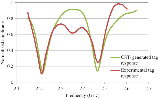
Figure 12.5 Tag response for [1010].
An 8-bit MIMO tag was fabricated to have tag bits [1010] in the first branch and [0000] in the other. An AWG was used to generate the interrogating signal at 2.4 GHz and oscilloscope with 20 GSamples/s was used to capture the tag responses available at each branch. ML-based tag detection was performed only on the first branch for demonstrative purposes and the same technique can be applied to the second branch too. Table 12.1 shows the distance value obtained for each tag type after evaluating the expression in (12.14). It can be clearly seen that minimum distance occurs at the tag type [1010] as highlighted in Table 12.1. A comprehensive analysis was carried out using MATLAB simulations, as it is not feasible to take large number of experimental data.
Table 12.1 An Example of a Table
| Tag Type | Distance in (12.14) | Tag Type | Distance in (12.14) |
| [0000] | 10.84 | [1000] | 4.73 |
| [0001] | 7.57 | [1001] | 4.12 |
| [0010] | 5.03 | [1010] | 0.56 |
| [0011] | 7.89 | [1011] | 2.80 |
| [0100] | 4.49 | [1100] | 1.62 |
| [0101] | 3.58 | [1101] | 2.75 |
| [0110] | 3.51 | [1110] | 2.61 |
| [0111] | 5.74 | [1111] | 5.29 |
12.5 SIMULATIONS
Simulations were carried out in two methods. In the first method, tag responses were generated in MATLAB using bandstop filters. The interrogating signal was generated using orthogonal frequency division multiplexing (OFDM) techniques. The MIMO decomposing technique explained earlier was implemented in MATLAB and the tag responses in each branch of the MIMO tag were estimated. In this method, tag detection was performed using a threshold-based valley detection technique applied on the power spectral density (PSD) of the estimated tag responses. This information was used to calculate the DER at different SNR levels.
In the second method, both the interrogating signals and the tag responses were generated using CST simulations. The MIMO decomposing technique and the tag detection technique described in the previous section were implemented in MATLAB. Finally, the DER at different SNR levels was calculated. First, the details about the first method are described next.
12.5.1 METHOD 1
The signal path from the RFID reader through the MIMO tag back to the reader was modeled in MATLAB using the baseband signal representation. As briefly explained earlier, in this method first the interrogating signal is generated using OFDM techniques. This was achieved using binary phase shift keying (BPSK)-modulated test bits. All 200 test bits were selected as “1.” Other OFDM parameters used in MATLAB simulations are displayed in Table (12.2).
Table 12.2 Simulation Parameters
| Parameter | Value |
| Number of BPSK modulated of test symbols | 200 |
| OFDM block size | 25 |
| Length of cyclic prefix | 2 |
| Number of FFT / IFFT points | 25 |
| Sampling frequency | 600 MHz |
| OFDM signal bandwidth | 300 MHz |
| Total bits encoded in the tag | 6 bits |
| Bandstop filter attenuation | 10 dB |
| Number of branches in the MIMO tag | 2 |
| Resonance frequency set (MSB to LSB) | [50, 150, 250, 350, 450, 550] MHz |
Then the resonators were emulated using bandstop filters in MATLAB and the filter attenuation was selected as 10 dB. Center frequencies of the bandstop filters were selected as shown in Table 12.2. Multiple resonators were emulated using cascaded bandstop filters. Then the tag responses were fed through a channel that is given by the product of the forward and reverse channels of the RFID system. In the MATLAB simulations, the channel is assumed to be known at the RFID reader. Finally, noise was added to the resultant signal according to the specified SNR.
Baseband signals received at the RFID reader was used for MIMO decomposing. Then ZF equalizer was used to decompose the received signal and obtain an estimate of the tag response in each branch. Then a threshold-based valley detector was used to identify the presence and absence of resonators, which will be used to read the encoded tag data bits. Finally, the DER was calculated for each tag detection technique at different SNR levels.
Figure 12.6 illustrates the flowchart of the MATLAB simulation carried out. However, the calculation of tag responses using bandstop filters does not take into account any coupling between the two branches in the tag. Therefore, a more realistic simulation was performed using CST. In addition, valley detection technique used to identify the tag data bits is very primitive and can be further improved using advanced tag detection techniques. The second method explained in the following section rectifies these limitations.

Figure 12.6 Flowchart of the MATLAB simulation.
12.5.2 Method 2
As explained in the previous section, method 2 uses CST to simulate tag responses, which takes into account any coupling between the two branches in the MIMO tag. The tag responses generated using CST simulations are more realistic than bandstop filter emulation performed in the previous method. Then the validity of the tag detection technique derived in Section 12.3 was verified using MATLAB.
The steps carried out in the simulation are given in Figure 12.7. First, an interrogating signal was generated to provide a flat frequency response in the 2.2–2.6 GHz frequency range. Four resonators were designed using CST with resonating frequencies as shown in Table 12.3. Then the combinations of resonators were placed beside a microstrip line to cover all possible tag IDs. One end of the microstrip line was fed with the interrogating signal and the tag responses were collected at the other end. These collected tag responses were saved in a lookup table for the algorithms to be used later.

Figure 12.7 Flowchart of the MATLAB simulation.
Table 12.3 Simulation Parameters
| Parameter | Value |
| Center Frequency | 2.4 GHz |
| Total bits encoded in a tag | 4 bits |
| Flat frequency response | 400 MHz |
| Bandstop filter attenuation | 10 dB |
| Guard band | 50 MHz |
| Resonance frequency set (MSB to LSB) | [2.2, 2.3, 2.4, 2.5] GHz |
| Number of iterations | 1,000,000 |
Then the signal flow from the MIMO tag to the reader was modeled in MATLAB and the channel information was assumed to be available at the reader. ZF equalizer was used to decompose the tag responses in each branch of the MIMO tag. Then the tag detection technique derived in Section 12.3 was used to identify the encoded tag data bits. Finally, the detection error rate was calculated at different SNR levels. The results obtained in each simulation method are discussed next.
12.6 RESULTS
In this section, results obtained using the two simulation methods are presented. First, the results of the method using OFDM technique and bandstop filters are discussed.
12.6.1 Method 1
In the simulation, the test bits are selected as all ones and they are BPSK modulated. Then the BPSK-modulated signals are OFDM modulated to generate the interrogating signal in time domain as shown in Figure 12.8. When the test bits are taken as all ones, the resulting interrogating signal will be similar to having a train of impulses.

Figure 12.8 Interrogating signal in time domain.
The two-sided PSD of the interrogating signal is shown in Figure 12.9. It can be considered that the signal has a flat frequency response throughout the signal bandwidth of 300 MHz.

Figure 12.9 Two-sided PSD of the interrogating signal.
This interrogating signal was then transmitted through a SISO channel to the tag and the time-domain representation of the received signal is shown in Figure 12.10.

Figure 12.10 Received signal at the tag.
Then the received signal at the tag is divided into two equal RF components and each component will travel surrounding spiral resonators. The spiral resonators were implemented as bandstop filters in MATLAB and Figure 12.11 shows the filter response of such a spiral resonator. Altogether three resonators were emulated at 47, 150, and 253 MHz. The presence of a resonator was represented as bit “1” while the absence as bit “0.” As there are two components that are tag modulated independently, the considered prototype has a capacity of 6 bits.

Figure 12.11 Filter response of a spiral resonator.
Once each component reaches its transmitting antenna, it contains the frequency signature of all the spirals presented along the way. Figure 12.12 shows the two-sided PSDs of each signal (Tx1 and Tx2) after traveling via spiral resonators. Top graph in Figure 12.12 represents the case of having only two resonators at 47 and 253 MHz (corresponds to [101]) while the bottom represents having three resonators at 47, 150 and 253 MHz (corresponds to bits [111]). Presence and absence of the spiral resonators in each branch can clearly be observed.

Figure 12.12 Two-sided PSD of the tag-modulated signals (Tx1 and Tx2).
The time-domain representation of the above two signals is shown in Figure 12.13. The noise introduced by the receiving tag antennas is visible at the two signals already.

Figure 12.13 Tag-modulated signals (Tx1 and Tx2) in time domain.
Then the two transmitted signals were propagated via a ![]() MIMO channel. Figure 12.14 shows the channel realizations for both forward and reverse channels. As a result of Rician distribution, the four MIMO channel realizations looked very similar. After being mixed with the channel, the received signals at the receiver antenna array are shown in Figure 12.15.
MIMO channel. Figure 12.14 shows the channel realizations for both forward and reverse channels. As a result of Rician distribution, the four MIMO channel realizations looked very similar. After being mixed with the channel, the received signals at the receiver antenna array are shown in Figure 12.15.

Figure 12.14 Channel realizations.

Figure 12.15 Received signals at the two Rx antennas of the reader.
The received signal array were then decoded using MMSE equalizing method and the estimated transmitted signals (Tx1H and Tx2H) were obtained. Figures 12.16 and 12.17 compare the actual and the estimated transmitted signals in time domain for Tx1 and Tx2, respectively. It can be observed that the estimates are very similar to the actual signals.

Figure 12.16 Actual and the estimated Tx1.

Figure 12.17 Actual and the estimated Tx2.
The two-sided PSDs of each of the estimated transmitted signals (Tx1 and Tx2) are shown in Figure 12.18. A separate algorithm was implemented to detect the presence and absence of the frequency dips at the resonating frequencies. Using the algorithm, estimated data bits were obtained and were compared with the data bits encoded in the tag.

Figure 12.18 Combined tag response.
The simulation was repeated for 100 times, and Figure 12.19 shows the combined tag response obtained for 100 iterations. It can be concluded that for different channel realizations, the performances are consistent.

Figure 12.19 Combined tag response for 100 iterations.
Simulations are carried out to investigate the bit error rate (BER) performance under different signal-to-noise ratios (SNRs). SNR is defined as the signal-to-noise ratio at each of the receiving antenna array at the reader. Figure 12.20 shows the BER performance of the proposed system versus SNR and also a comparison to the theoretical BER of a traditional binary phase shift keying (BPSK) modulation scheme. Even though, the definition of the BERs in two schemes is different, it is interesting to learn that the simulated system performances closely follow the theoretical BER performance for a BPSK-modulated ![]() MIMO system. In traditional BPSK modulation schemes, the bits are modulated into either raised cosine symbols or no signal at all based on the bit value. In the PSD, it is similar to be represented using the presence and absence of a valley. As a result, the two schemes can be compared and should display similar performance which they do.
MIMO system. In traditional BPSK modulation schemes, the bits are modulated into either raised cosine symbols or no signal at all based on the bit value. In the PSD, it is similar to be represented using the presence and absence of a valley. As a result, the two schemes can be compared and should display similar performance which they do.

Figure 12.20 BER of the proposed system versus SNR.
Figure 12.21 shows a comparison between the proposed ![]() MIMO system and the traditional SISO multiresonator-based chipless RFID system. In this simulation, the same data bits were encoded in both the branches introducing diversity. Compared with the traditional system, it is evident that the two branches in the MIMO multiresonator tag cause less errors due to the extra reliability in the proposed system. This extra reliability can also be seen differently as encoding more data bits in the tag with an acceptable reading accuracy. Apart from that, the diversity gain of the MIMO system is clearly visible compared to linear variation in the SISO system.
MIMO system and the traditional SISO multiresonator-based chipless RFID system. In this simulation, the same data bits were encoded in both the branches introducing diversity. Compared with the traditional system, it is evident that the two branches in the MIMO multiresonator tag cause less errors due to the extra reliability in the proposed system. This extra reliability can also be seen differently as encoding more data bits in the tag with an acceptable reading accuracy. Apart from that, the diversity gain of the MIMO system is clearly visible compared to linear variation in the SISO system.

Figure 12.21 Noise performance of the proposed system versus SISO counterpart.
12.6.2 Method 2
The results obtained using both CST and MATLAB simulations are presented and discussed in this section. The resonator response simulation is similar to that of the SISO tag simulation. Figure 12.22 shows the resonator response of a branch when all four resonators are presented. It can be clearly seen that the four resonances at the designed frequencies 2.2, 2.3, 2.4, and 2.5 GHz.

Figure 12.22 CST-generated tag response for a branch having [1111] tag bits.
The received signal at each receiving antenna of the reader is calculated using (12.9) under different noise power levels. Then the received signal array is decomposed using ZF decoder as shown in (12.7) to calculate the estimated tag responses in each branch. Finally, the likelihood-based detector derived in (12.14) is used to identify the tag data bits. Figure 12.23 compares the DER against SNR for the two methods.

Figure 12.23 Comparison of DER performances for 6 bit tags.
It can be clearly seen that the likelihood-based detection technique (method 2) is performing better than the valley detection-based technique in method 1. For example, at ![]() , method 1 has a DER of 99.8%, while method 2 produces an accuracy of 99.99%. At higher SNR levels, both methods perform better for obvious reasons. It can be concluded that the likelihood-based detection method performs better than the valley detection method at all SNR levels. However, method 2 assumes perfect channel state information. In case if there are errors in channel estimation, it could magnify the noise amplitude with ZF decoder and performances could be degraded.
, method 1 has a DER of 99.8%, while method 2 produces an accuracy of 99.99%. At higher SNR levels, both methods perform better for obvious reasons. It can be concluded that the likelihood-based detection method performs better than the valley detection method at all SNR levels. However, method 2 assumes perfect channel state information. In case if there are errors in channel estimation, it could magnify the noise amplitude with ZF decoder and performances could be degraded.
12.7 CONCLUSION
This chapter presented signal processing techniques for successfully detecting the tag bits of a MIMO-based chipless RFID system. First, ZF decomposing techniques were used on the received data array at the reader to estimate the tag response. Then two methods were used to detect the tag data bits encoded in the MIMO tag. The first method uses a threshold-based valley detection method. The other method uses the proposed ML detection technique to detect the tag bits in each branch of the MIMO chipless tag. An experiment was set up to test the ML detection technique and it was shown that the encoded tag data bits are identified successfully. In order to perform a comprehensive analysis, CST- and MATLAB-based simulations were performed. The results show that the proposed detection technique provides better detection error rate performance at different SNR values over traditional threshold-based detection. This benefit can be interpreted in two different metrics. First, it can be seen as an SNR gain over the existing threshold-based detection technique, which effectively increases the reading range. Second, the high accuracy in tag reading avoids multiple reading cycles, which yields an energy-efficient reading method.
Theoretically, higher number of branches can encode higher tag data bits within the same frequency band. However, the number of receiving antennas used in the reader should be always equal to or higher than the total branches in the MIMO tag to successfully decompose the signals. In addition, due to short distance the proposed setup operates under line-of-sight (LOS) MIMO. In LOS MIMO, the physical distances between antennas have to be maintained such that they will not form similar channel gains between transmitter and receiver antennas. As a result, the maximum number of branches allowed in the tag is limited. Main drawback of ML detection technique is computation complexity. It was demonstrated in Chapter 11 that the proposed computationally feasible detection techniques reduce the complexity from exponential to linear order without compromising the tag reading accuracy.
REFERENCE
- 1. C. Divarathne and N. Karmakar, “MIMO based chipless RFID system,” in RFID-Technologies and Applications (RFID-TA), 2012 IEEE International Conference on, Nov 2012, pp. 423–428.