
CHAPTER 7
FAST IMAGING THROUGH MIMO-SAR
7.1 INTRODUCTION
Providing a fine spatial resolution on the chipless RFID tag surface through the millimeter-band 60 GHz and synthetic aperture radar (SAR) technique has been introduced earlier. While the proposed technique benefits from many practical features, there are two main issues that deter its full potentials. The requirement for relative movement of the reader and tag is recognized as the most crucial limitation of the proposed technique. Moreover, the tag orientation sensitivity is also associated with the proposed technique, while a practical solution has been suggested in the previous chapter. This chapter considers the requirement for movement of the reader and a practical solution with reasonable hardware complexity is suggested.
The general structure of the proposed technique based on the conventional SAR technique is shown in Figure 7.1. The reader, including its two orthogonally oriented antennas, moves around the tag and captures the backscattered signal at different view angles. The total synthetic length depends on the reading range, required image resolution, and the tag data capacity. However, as shown in the previous chapters, the maximum length of 30 cm is enough to provide 0.5 image resolution when the tag has its maximum length, 8.5 cm. The interval between each two adjacent transmit and receive antennas also depends on the wavelength. Normally, 2 mm is selected as the physical separation between two transmissions as shown in Figure 7.1.

Figure 7.1 System structure of the proposed spatial-based approach.
Therefore, one may conclude that 100–150 individual transmit and receive reading process is normally required. As addressed before, this is a long reading process that is not obviously practical for the current applications of chipless radiofrequency identification (RFID) systems.
This chapter is organized as follows: (i) the phased array antennas with agile beamforming capability are considered as a solution for reader movement and its system complexity is discussed. (ii) The new idea of multiple input multiple output (MIMO)-based array antenna is presented. (iii) MIMO-based array antenna is designed for fast imaging of the tag and the result of simulation is presented. (iv) Finally, the approach for optimization of the MIMO-based system is introduced for minimum number of antennas.
7.2 CONVENTIONAL PHASED ARRAY ANTENNA
Phased array antennas have emerged as the most advanced technology in the modern-day radar systems. It provides huge enhancement in features that are of interest in radar systems, modern wireless communications, and many commercial applications. In a phased array antenna, antenna elements are precisely controlled in relative excitation of phase and amplitude to generate directional beams and nulls in desired direction [1].
Appropriate relative phase adjustments of the array elements in the time domain is known as the time-domain beamforming. This happens by creating precise time delays in the received signals of each array element. Time-domain beamforming provides an accurate result for a wideband signal; however, the precision of the delays is restricted to the capabilities of devices for precise time-delay control. It is also possible to use the fast Fourier transform (FFT) and transfer the required adjustment of the array elements in frequency domain instead of time domain. In this scenario, a proper phase shift in each adjacent element is required instead of time delay. This means that through specific phase shift in the feeding route of each array element, the array can steer on a specific direction. Solid-state digital phase shifters and voltage variable controlled attenuators are widely developed nowadays on which precise adjustment of each antenna element based on the required “weight vectors” is possible. The frequency domain is a more common technique in the phased array systems than the time-delay approach as it can provide much more accurate beamforming results.
Applying the phased array antenna theory to the proposed image-based chipless RFID system, two difficulties should be considered. First, in the phased array structure, phase shifters or their equivalent time-delay modules are needed. To precisely scan the tag surface in the order of a few millimeters, the phase shifters' granularity will be very fine [2, 3]. Utilizing accurate phase shifters in the 60 GHz frequency band significantly increases the system cost. Moreover, when the phased array antenna scans the tag, the beam shape distorted with the view angle. This may not be a serious issue in many applications; however in the proposed theory, the fixed shape of the radiation pattern is vital, otherwise, the tag's image is distorted [4].
To minimize the variation of the agile radiation pattern at different view angles, it is possible to use a very accurate feeding algorithm that provides the required amplitudes and phase shifts to individual elements [2]. In this approach, more accurate amplitude tapering modules and precise phase shifters are required that significantly increase the system's cost and complexity [2]. Therefore, phased array antennas with fixed beam shape are normally restricted to very-high-technology military applications. The proposed low-cost EM-imaging chipless RFID system cannot tolerate such an expensive and complex antenna system.
With the aforementioned limitations, it can be concluded that the usage of a conventional phased array antenna for replacement of the moving reader is not practically feasible for the RFID application. Therefore, an alternative to the conventional phased array antenna – a MIMO-based array antenna with reduced complexity – is considered next.
7.3 MIMO-SAR SYSTEMS
MIMO refers to a system with multiple transmit and receive antennas for multiplying the capacity and performance of the radio systems by exploiting the spatial diversity. Considering the potential advantages on providing flexibilities and freedom due to the usage of multiple channels, the MIMO-based systems are of interest to researchers [5]. MIMO technique has recently provided noticeable simplifications on radar systems [6–8]. MIMO-SAR employs multiple antennas to transmit orthogonal waveforms and multiple antennas to receive radar echoes. MIMO-SAR is recently proposed in remote sensing concept [9]. It is shown that the MIMO-SAR can be used to improve the remote sensing system performance. One of the main advantages of the MIMO-SAR is greatly increased degrees of freedom by the concept of virtual antenna array [6]. In a conventional phased array radar system, the transmitted signals are inherently dependant. They only vary by some time delays or equivalent phase shifts. However, in the MIMO-based system, each antenna transmits a unique waveform that is orthogonal to the waveforms transmitted by other antennas. This means that the return signals to each receive antenna element will carry independent information about the target, hence increasing the system's freedom and flexibility. The phase difference caused by different transmitting antennas along with the phase differences caused by different receiving antennas can form a new virtual antenna array steering vector [6]. With optimally designed array elements' positions, a very long array steering vector with a small number of antennas can be created. This provides high flexibility and reconfigurability in antenna configuration [6, 10].
The idea of the MIMO-based array antenna is applied on the chipless RFID system. It is found that the new technique of MIMO-SAR system has huge potential for enhancing the tag imaging time on a fairly low-cost and simple reader configuration.
7.3.1 MIMO-Based Array Antenna
An eight-element MIMO-based antenna including four transmit and four receive antennas is shown in Figure 7.2. Each of transmit and receive antennas can be viewed as a sparse array. The normalized separation distance between Rx and Tx antennas are 6 and 9, respectively, as shown in Figure 7.2. Dimension is not important, but centimeter can be assumed as example. Therefore, the sparse array antennas have constant separation of 3 cm. This means that the Rx array is equivalent to a sparse array of seven elements with a separation distance of 3 cm and the active and passive elements distribution of
| 1 | 0 | 1 | 0 | 1 | 0 | 1 |

Figure 7.2 MIMO-based antenna system and the equivalent sparse array antennas.
The same assumption is valid for the Tx array with the following topology for the active and passive elements and again with a separation distance of 3 cm:
| 1 | 0 | 0 | 1 | 0 | 0 | 1 | 0 | 0 | 1 |
It is envisioned to show the transition between the MIMO theory and its equivalent virtual array antenna without being deeply involved with the mathematical calculations [11]. In Figure 7.2, each Tx antenna can independently transmit its signal and all the Rx receive antennas collect the backscattered signal. Based on the array theory, it can be shown that the array factor of each array antenna is equivalent to a polynomial of N − 1 order on which N is the number of array elements [12, 13]. Therefore, the related polynomials of receive and transmit arrays are as follows, respectively:

It can be mathematically proven that the two sets of Tx and Rx antennas on MIMO-based configuration is equivalent to a virtual array antenna. This means that instead of analyzing the MIMO-based antenna, one may consider the equivalent virtual array and expect almost the same radiation characteristics as the MIMO-based antenna. The details of expressions for relation between the MIMO-based system and the virtual array are not discussed here. It has been shown that the convolution of the Tx and Rx arrays defines their equivalent virtual array antennas and subsequently specifies the position of the active elements in the virtual array configuration [6, 11]. Therefore, two sets of the Tx and Rx antennas that have been considered as sparse arrays are mathematically linked to their virtual array antenna. Based on this assumption, the convolution of the Tx and Rx antennas in the time domain is equivalent to multiplication in the frequency domain. Hence, one may simply find the equivalent virtual array's polynomial through the following relation [6]:

where Pv is the polynomial of the virtual array. This polynomial that is in the order of 15 relates to a 16-element linear array with the following active/passive topology:
| 1 | 0 | 1 | 1 | 1 | 1 | 1 | 1 | 1 | 1 | 1 | 1 | 1 | 1 | 0 | 1 |
In the above configuration, “0” means that position has no antenna and “1” represents an active antenna. The bold “1” show duplicate element position. With this procedure, the MIMO-based structure of 4 + 4 physical elements is related to a virtual array of 4 × 4 elements. The actual MIMO based system and its equivalent virtual array antenna are presented simultaneously in Figure 7.3, in which the physical MIMO-based system and its equivalent virtual array antenna are presented simultaneously.

Figure 7.3 MIMO-based antenna and its equivalent virtual array antenna.
To have a more physical sense of evolution from MIMO-based system to the array antenna concept, one can track the signal route when it is transmitted by a specific transmit antenna (Ti) and received by all receive antennas. Let consider dr and dt as the separation distance between the Rx and Tx antennas, respectively. The relative position of each Tx antenna to the center point of the transmit array antenna is denoted by dtn and the relative position of each Rx antenna to the center point of receive array is shown by drm, where m, n = [1, 4].
When one of the transmit antennas is active, then the received signals to all receive antennas can be weighted by
This clearly shows that the relative positions of each set of transmit and receive antennas and the relative phase shift in its equivalent virtual array. To establish a unique phase center for all communication links between the transmit and receive antennas, one can shift the position of transmitters to a fixed point, the center of transmit array, for instance, and then find the phase shift occurring in all receive array elements. This is shown for the two cases of T1 and T2 in Figure 7.4. While T1 antenna is dt1 shifted to the right side, all its related Rx antennas are equivalently shifted to the left side for the same distance. The same happens for case T2. However, the distance of movement is now dt2. If the shifted Rx antennas for these two cases are mapped to each other, they fill the gaps among physical elements. This is shown in Figure 7.4 by the dashed arrows and circles among active antennas. If the same procedure continues for T3 and T4, then the virtual array element is completed and would be similar to the declared virtual array polynomial and the position of the antenna in the virtual array as follows.
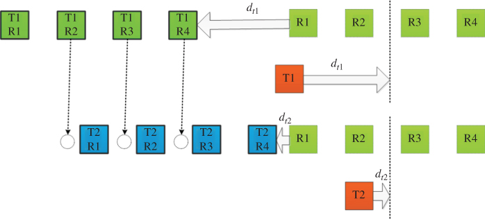
Figure 7.4 Relative phase shift between one particular Tx antenna and all Rx antennas.
7.3.2 MIMO-SAR Array for Chipless RFID Imaging
To design the MIMO-based phased array antenna for the proposed chipless RFID system, the process described in Ref. [14] is followed. In the proposed configuration, every two Rx antennas are linked with five Tx antennas. Then the structure is cascaded to provide the larger required equivalent array antenna. Figure 7.5 shows the structure of this MIMO-based antenna configuration. It is important to find the relation between the separation distance of Rx and Tx antennas and their equivalent virtual array. The angles θ1 and θ2 can be linked to other parameters as follows:
where the parameters of (7.4) are defined in Figure 7.5. To find the position of the points a and b, one can write the following expressions:


Figure 7.5 MIMO-based antenna and its equivalent virtual array.
Therefore, the separation distance of Rx antennas can be easily linked to the separation among the virtual array elements, ΔXv, through
If the same approach is followed for θ3 and the distance between points b and c is found, one can easily reach the following relation:
We have already discussed that the reader antenna has to illuminate the tag in every 2 mm. Therefore, the inner space of virtual array element shall be 2 mm and equivalently, the physical Rx antennas have to be 4 mm and Tx antennas 8 mm apart from each other.
The total number of sampling points also governs the total number of required physical antennas. We have already discussed that “m + n” elements in Rx and Tx configuration may provide a virtual array of “m × n” elements. It is important to mention that this is a theoretical criterion and shows the minimum number of required actual Tx and Rx antennas. For example, 8 and 13 physical antennas are utilized in Ref. [14] for a virtual array with only 44 elements while based on the theoretical relation, less number of antennas are expected for the virtual array with 44 elements. For the case of RFID application, it was shown earlier that the reader shall stop in 100–150 individual points and illuminates the tag and capture the backscattered signal. Thus, the average number of virtual array elements can be assumed as 125 points; however, it is possible to have slightly higher or even less number of array elements. Therefore, 125 points can be seen as a rough estimate. The proposed MIMO-based system topology for the Rx antenna in Ref. [14] includes two active antennas and then four passive elements in the sparse array configuration, 11000011 array polynomial. The Tx array has one active and one passive element scheme, 101010, for instance. Based on this assumption, the antenna distribution scheme is as follows:
- For Tx array antenna: 11000011000011000011
- For Rx array antenna: 1010101010101010101010101
Based on this array distribution, the following polynomials can be related to the Rx and Tx antennas, respectively, for the 44 elements requirements:
Obviously, the convolution of the above polynomials results in a virtual array of degree 43. If the same topology is followed for the case of 125 array elements, one may suggest the following polynomial for the Rx array antennas including 24 active antennas:

Based on the above assumption for the Rx configuration, the related Tx antennas can be defined through the following polynomials with 31 physical Tx antennas:

The convolution of (7.9) and (7.10) results in a polynomial of degree 127, which includes all the required elements.

In Equation (7.11), coefficients ai may be different from “1.” In this case, it is not required to consider all relevant combinations between an individual Tx and Rx antennas. Therefore, through (31 + 24) physical antenna, it is possible to implement a virtual array with 127 elements. Through this configuration, the total number of array elements drops from 127 × 2 = 254 to only 31 + 24 = 55 elements. Moreover, the reading time in the proposed technique would significantly enhance while no complex system structure is utilized. The conventional SAR technique through physical antennas and its equivalent MIMO-SAR are shown in Figure 7.6. In the conventional SAR, a pair of Tx and Rx shall move around the tag and stop in 127 positions and perform the reading process. Equivalently, 127 pair of antennas can be used for fast reading process. However, in the MIMO-SAR technique, only 55 physical elements are utilized with no requirement for physical movement of antennas.

Figure 7.6 Conventional SAR and MIMO-SAR in a glance.
The summary of the MIMO-based system can be compared with a physical array and the conventional SAR technique as mentioned in Table 7.1. The conventional SAR technique has the minimum system complexity due to the usage of only one antenna pair. However, it provides a very slow imaging process in conventional approach or fairly slow imaging speed if a stepper motor is utilized. It is possible to develop an array antenna for fast imaging process while it requires a large number of elements, which results in significant system cost. Instead, one may use the MIMO-SAR system with much lower number of elements and the requirement for a switching network.
Table 7.1 The MIMO-Based Advantages
| Number of Elements | System Complexity | Imaging Time | |
| MIMO-based antenna | M + N(min) | Switching network | Fast |
| Array antenna | M × N | Phase shifter/amplitude tapering | Fast |
| Conventional SAR | 1 | Physical antenna movement | Very slow/slow (stepper motor) |
7.3.3 Simulation Result
Figure 7.7 shows the proposed structure of the MIMO-based system. 24 Rx antennas with 4 mm separation distance are linked with 31 Tx antennas with a separation distance of 8 mm. Hence, the total aperture size is less than 25 cm (31 × 0.8 = 24.8 cm) that is completely matched with the aperture sizes introduced before. The virtual array antenna with 127 elements is located between the Rx and Tx antennas. No phase shifter or amplitude tapering network is required. Only a switching network is utilized to connect one Tx antenna with its associated Rx antennas at a time.

Figure 7.7 MIMO-based antenna for EM-image-based chipless RFID system.
To test the validity of the proposed technique of a MIMO-based reader, a 6-bit tag is selected as example. The tag's image is simulated through a MIMO-SAR system and then compared with the image through normal SAR technique. The result of signal processing is shown in Figure 7.8. In the SAR technique that includes 125 individual send and receive process, the EM image adequately shows the encoded data. If the same tag is processed through a MIMO-SAR system that utilizes 55 physical antennas, then the image is depicted in Figure 7.8(c). The EM image seems to be somehow noisier than that for the conventional SAR. Moreover, the imaged column of meander lines shows a minor inclined nature so slightly degrades the azimuth resolution. One reason may be suggested for the degraded image of the tag through MIMO-SAR technique. The equivalence between the virtual antenna and its associated MIMO system is an approximated relation. Each set of Tx and Rx antennas is associated with one single element in the virtual array. However, based on the physical distance of Tx and Rx antennas, a certain amount of error due to the phase center is expected. This error is reflected in the nonperfect image of the tag through MIMO-SAR technique. However, much faster imaging time of MIMO-SAR system compensates the noisier image of the tag. Moreover, it is possible to use higher number of physical antennas on the MIMO-based system and improve the image quality. Alternatively, by optimization of the antennas distribution on the MIMO-basis system, one may expect a higher quality of the imaged tag. The optimization process of the antennas distribution in the MIMO-SAR system is introduced in the following section.

Figure 7.8 Photographs of (a) printed 6-bit tag, (b) tag image through normal SAR, and (c) tag image through MIMO-SAR technique.
7.4 OPTIMIZATION
As discussed in the previous section, the usage of 24 Rx and 31 Tx antennas is based on the suggested topology in Ref. [14] on which 2 Rx and 5 Tx antennas are connected to each other. Then the structure can be expanded by cascading them to provide the required aperture size. This scenario is also based on the linear sparse array theory assumption. Obviously, the number of utilized antennas, 55 elements, is not easy to implement and may put restriction on the practicality of the proposed MIMO-based approach. Moreover, the expectation is to have a virtual array of 127 elements with much lower number of physical Tx and Rx antennas, 11 + 12 elements, for example. This simply means that the proposed topology in Ref. [14] is not optimum and it would be probably possible to reduce the number of actual antennas and still expect the same virtual array size. To optimize the MIMO-SAR system for the minimum number of physical antennas, two approaches can be considered: analytical and numerical optimization approaches.
7.4.1 Analytical Approach
First, it is suggested to represent the problem analytically and explore if there is any mathematical approach to find the minimum number of physical antennas in the MIMO-SAR configuration. The aforementioned situation for the MIMO-SAR can be analytically shown as

In the above set of expressions, the product of Pr × Pt shall produce a complete polynomial of order “n.” The number of active elements in the Rx and Tx series is shown by “k” and “t,” respectively. There are some other limitations that shall be considered in the optimization process. First, as it is mentioned before, the relation between any Tx and Rx antennas with their equivalent virtual element is an approximate relation. This relation is more accurate if the distance between the Tx and Rx antennas is negligible with respect to the distance of the target in front of the antennas. This implies an additional limitation in the above sets of formula in Equation (7.12). Every Rx antenna shall be connected to its neighboring Tx elements and not to the Tx antennas that are physically located far from the intended Rx antenna. Otherwise, the results of analytical optimization may be mathematically accurate but results in a system with inaccurate performance. Second, the goal is to minimize k + t, while it is also desirable to have the minimum physical space occupied by the MIMO-based system. The other parameters of the system shall also be considered in the above sets of formula. Considering the limitations set out for the optimization problem, any analytical approach would be very complex if any existed. The authors are not aware of any analytical approach for solving the above-described problem.
7.4.2 Numerical Optimization Process
The second approach is the numerical optimization process. In the analytical approach, the suggestion is to consider the distribution of the Tx and Rx antennas as a uniform sparse array antenna for simplicity. In the numerical approaches, however, such a suggestion is not mandatory. This means that nonuniform sparse array structures can also be considered, which may result in a lower number of antennas or smaller array size.
Before selection of any specific optimization technique, it is useful to explore the dimension of the problem. This helps selecting the best technique with least complexity. The maximum length of the demanded virtual array for the proposed application, as discussed before, is 30 cm. It is necessary to find out what is the length of Tx and Rx arrays in the MIMO system. Referring to Figure 7.3 and by following the approach of shifting the Rx array for the relative position of each Tx antenna, as described in Section 7.3.1, one may easily prove
where RL, TL, and VL are the physical length of Tx, Rx, and virtual array, respectively. To find out RL and TL, another equation is required. This means that the relative length of Tx and Rx arrays should be known. Although no specific relation can be defined for the length of Tx and Rx arrays, the ratio of RL to TL that has been suggested by Lincoln Laboratory [11] may provide a practical value:
Considering Equations (7.13) and (7.14), one may easily find the total length of Rx and Tx as
The maximum length of the virtual array is 30 cm and it was already shown that the reading process shall be occurred in each 2 mm. Therefore, one may see the virtual array as a uniform array of 150 elements with a uniform distribution and an element spacing of 2 mm. Referring to Figure 7.5, the minimum element spacing of the Rx and Tx arrays shall be 2 mm or lower. For simplicity of optimization, the 2 mm is selected. Consequently, the Rx and Tx arrays on MIMO basis can be viewed as nonuniform sparse array of 60 (12 × 5) and 90 (18 × 5) elements. The total number of physical antennas on Tx and Rx is restricted by
on which k and t are the total number of real Rx and Tx antennas as already defined in Equation (7.12). A good suggestion for k and t would be 11 and 14, respectively. Therefore, the optimization problem has been simplified as follows.
The total number of 11 and 14 antennas will be distributed appropriately on sparse arrays with 60 and 90 elements, respectively, on which two arrays are connected on MIMO basis. The distribution of antennas on each array will be in such a way to result in a complete virtual array of 150 elements. Therefore, the total possible option for each case is as follows:

Therefore, the total number of possible cases would be more than 1045. This shows very wide dimension of the answer region for the suggested problem. Obviously, it would not be possible to verify all the possible cases even with the most advanced computer systems. Instead, an efficient optimization process is required to find the solution in a reasonable time frame.
Luckily, this is a common issue nowadays in many research fields, problems with widely extended feasible region without any known classical approaches. Applying the numerical techniques seems to be the only possible method. Moreover, classical numerical methods fail to provide solution in many cases as the target function does not have specific characteristics, being a continuous function or having derivatives, for example. In such cases, global optimization approaches are usually the best option. Another benefit of global optimization approach is their ability on finding the global optimum of a function. One of the main downsides of the classical optimization techniques is their failure on finding the best possible solution for a certain problem as they can easily be entrapped in local minima. Moreover, these techniques cannot generate or even use the global information needed to find the global minimum for a function with multiple local minima. The results of classical optimization approaches normally depend on the initial suggestion or starting point.
Mentioning the drawback of the global optimization techniques, one may refer to their computationally costly process due to the slow convergence. This means that irrespective of their significant ability of directing the optimization process toward the global optimum solution, they are normally inefficient to find the final answer. One of the main reasons for their slow convergence is that they may fail to detect promising search directions especially in the vicinity of local minima due to their random constructions. Combining global optimizations with local/classical search methods is a practical remedy to overcome the drawbacks of slow convergence and random constructions of global optimization techniques, hybrid methods. The advantages of global approaches are used to direct the process to the vicinity of global optimum and a classical technique is normally added at the final stage of the search.
In the global optimization techniques, evolutionary algorithms (EAs) are an important subset that generate solutions to optimization problems using techniques inspired by natural evolution. There are many techniques in EA category in which the genetic algorithm (GA) is one of the most significant approaches with the most effective results for a wide range of problems. GA is specifically very effective if no real-time solution is required [2, 15]. GA is proposed for the current problem of MIMO-SAR technique. The rest of this section briefly introduces GA and some of its main functions. Readers are suggested to refer to special references on GA for more detailed information.
7.4.3 Genetic Algorithm
Genetic algorithm that is been inspired by natural evolution encodes a potential solution to a specific problem on a simple chromosome-like data structure and applies recombination operators to these structures so as to preserve critical information. There are some parameters and key components in GA that will be defined and introduced. The most important ones are as follows:
- Genes: Genes are the essential blocks of the GA that carry the genetic information of an individual. Normally, genes represent the coded version of the physical parameters.
- Chromosome (genotype): A chromosome is a certain set of genes with a known length that define a proposed solution to the problem that the GA is aimed to optimize.
- Population: A group of chromosomes is called population.
- Generation: GA works on a specific population at each specific time that is called generation.
- Parents: Two or more chromosomes from the current population that have been selected to transfer their genetic characteristic to the next generation.
- Children: Referring to a chromosome belonging to the next generation and is the result of crossover among parents in the current population.
- Fitness: It is a number that is assigned to a chromosome and shows how well the chromosome satisfies the requirement of the problem.
There are four main operators in GA that control the flow of optimization process. First is the transformation and mapping of the real problem to the chromosome environment. The chromosome space is normally a binary-type data that shows the parameters and variables of the real problem. Then a certain number of chromosomes are selected to create the current population. After the construction of a population, parents have to be nominated for getting the chance of preserving their critical information. Normally, chromosomes with the highest fitness will have more chance of being selected as parent. However, this does not mean that the weaker individuals should have no chance for passing their genes to the next generation. Parents then do crossover and create children that belong to the next generation. There is the possibility of mutation in the children genes as well. This process will continue until one chromosome satisfies the requirement of the problem or a certain number of generation is passed. The main block diagram of the GA is shown in Figure 7.9. Readers may refer to the special references [15, 16] for better and more detailed explanations about each operator of the GA.

Figure 7.9 General block diagram of the GA.
7.4.3.1 Chromosome and Population Structure for MIMO-SAR
As discussed before, Rx and Tx arrays are assumed as sparse arrays with minimum interelement of 2 mm and maximum length of 12 and 18 cm, respectively. Each of Rx and Tx is sparse array with 60 and 90 elements, respectively, which includes certain number of physical antennas. Therefore, each chromosome shows one possible distribution of the physical antennas on the Rx and Tx arrays. The dimension of each chromosome is selected to be a matrix of [1,150]. The first 60 elements show how the physical antennas are distributed on Rx array and the rest, elements 61–150, show the scattering of physical antennas on Tx sparse array. A sample of chromosome is shown in Figure 7.10.
| 0 | 0 | 1 | 0 | 0 | 1 | 0 | 0 | 1 | 0 | 0 | 0 | 0 | 0 | 0 | 1 | 0 | 0 | 0 | 0 |
| 1 | 0 | 0 | 0 | 0 | 1 | 0 | 0 | 0 | 0 | 0 | 0 | 0 | 0 | 0 | 1 | 0 | 0 | 0 | 0 |
| 1 | 0 | 0 | 0 | 0 | 0 | 0 | 0 | 0 | 0 | 0 | 0 | 0 | 1 | 0 | 0 | 1 | 0 | 1 | 0 |
| 1 | 0 | 0 | 0 | 0 | 0 | 0 | 1 | 0 | 0 | 0 | 1 | 0 | 0 | 0 | 0 | 0 | 0 | 0 | 0 |
| 0 | 0 | 0 | 1 | 0 | 0 | 0 | 0 | 0 | 0 | 1 | 0 | 0 | 0 | 0 | 0 | 0 | 0 | 0 | 0 |
| 1 | 0 | 0 | 1 | 0 | 0 | 0 | 0 | 0 | 0 | 0 | 0 | 0 | 1 | 0 | 0 | 1 | 0 | 0 | 0 |
| 0 | 0 | 1 | 0 | 0 | 1 | 0 | 0 | 0 | 0 | 0 | 0 | 0 | 0 | 0 | 0 | 0 | 1 | 1 | 0 |
| 0 | 0 | 0 | 0 | 0 | 0 | 0 | 1 | 0 | 0 |
Figure 7.10 Sample chromosome for the MIMO-SAR optimization, red values relate to Rx and black numbers show the Tx array.
In this figure, the first 60 numbers relate to Rx array and show how the physical antennas are distributed. “1” means that position in the sparse array contains an active/physical antenna and “0” shows a blank point on the sparse configuration. As one may notice, there are only 11 physical antennas on the Rx section and the rest are zeros. The same is true for the Tx array that is shown for elements 61–150 with 14 “1” showing the physical antennas.
The next step is to create the first population. If the size of population is selected to be 50, then 50 random chromosomes similar to the structure shown in Figure 7.10 will be created. Therefore, the population has the dimension of 50 × 150 as shown in Figure 7.11.

Figure 7.11 Structure of population in GA.
7.4.3.2 Fitness Calculation
Each individual/chromosome in the population suggests a certain arrangement of the physical antennas for the Rx and Tx array structures. It is required to evaluate and quantify the suitability of each individual by assigning a value as the fitness to each chromosome.
For calculation of the chromosome's fitness, the related polynomial for each of Rx and Tx arrays will be calculated. As an example, the related Rx and Tx polynomials for the chromosome of Figure 7.10 are as follows:

As mentioned before, the virtual array is the result of Rx and Tx convolution in the time domain or multiplication of their polynomials in the frequency domain. Therefore, two polynomials of Equation (7.17) are multiplied to result in:
In an ideal scenario, Equation (7.18) is a complete polynomial of order 149 without any zero coefficient. However, as the sample chromosome that resulted in Equation (7.18) is not the best individual, hence Equation (7.18) includes some zero coefficients.
Based on this, one may define the fitness in such a way to show the number of zero coefficients of the resulting polynomial for each chromosome. Therefore, the lower is the fitness means less number of zero coefficients and hence the better the chromosome.
After calculating the fitness of all individuals in the initial population, the chromosomes in the population are rearranged based on their fitness. The best chromosome, which has the lowest fitness value, goes to the top and the worst chromosome with highest fitness value will be located at the end of the population. This is required for selection operator, which is discussed in the following section.
7.4.3.3 Selection Operator
After arranging the population based on the chromosomes' fitness, some individuals are to be selected as parents. Obviously, chromosomes selected as parents will have the chance of transferring their genes to the next generation. The nonselected chromosomes will die and their genetic information no longer existed in the optimization process. Therefore, it is important to make sure that the algorithm provides a rational process for preserving the critical genetic information of all chromosomes by giving them enough chance of being selected as parents based on their fitness values. There are many suggested approaches for the selection operator, of which the most common approaches are introduced briefly in the following text.
- Population Decimation. This is the simplest strategy for selection of parents. After arranging the population based on the fitness, a random value for fitness is selected. All the individuals who have the fitness worse than the threshold will be deleted. The parents are selected randomly from the remaining individuals. Irrespective of the easy implementation process, this selection strategy deletes all the weak individuals without giving them any chance of participating in the formation of the next generation.
- Proportionate Selection. This is one of the most commonly used techniques for the selection operator. Sometimes, it is also referred to as roulette wheel approach. In this approach, the chance of selection of each individual relates to its fitness by
7.19

which fparents shows the fitness of ith parents. The implementation of this approach is similar to a roulette wheel on which each chromosome occupies a certain area on the wheel surface based on its fitness as shown in Figure 7.12. The proportionate technique is efficient for the case when the number of population is high enough. Otherwise, some errors are expected for low population sizes. Moreover, the weak chromosomes have a small chance of transferring their genetic characteristics to the next generation.
- Tournament Selection. The tournament approach is normally believed to be the most common technique for selection operators. First, a group of chromosomes are randomly selected from the current population. Then the best individual in the selected bunch is the winner and hence will be selected as parent. The selected group will be returned to the population and the process repeats again. Tournament technique provides a satisfactory GA performance and has simple implementation process.
Variable Window Width. The variable window is one of the most effective techniques for the selection operator [15]. After rearranging the population based on their fitness, a window with variable length is applied to the population. Hence, the best chromosome is located at the beginning of the window and the end of the window includes the weakest chromosome in the selected window. Then, one individual is randomly selected from the chromosomes in the window as parent. The function that controls the window width is very important in this approach, and the total performance of the algorithm highly depends on this function [2]. The formula that has been suggested in Ref. [15] is as follows:
-
where W(L) is the window width, Int shows the integer value of the parameter, Pop is the total population number, L is a random value that controls the window width, and t is a parameter that has to be selected in such a way to create Wmax = Pop. Implementing the abovementioned procedure for the selection process, however, did not result in satisfactory operation of the algorithm. Investigating the proposed formula for the selection operator reveals the reason for this unsuccessful performance. If Equation (7.20) is plotted as shown in Figure 7.13, one may notice the reason. For most of the cases (L > 0.2), the first 25 chromosomes are having the same chance of being selected as parent. The first chromosome and the 25th individual normally have noticeable fitness value differences. This is almost inconsistent with the overall expectation from selection operator.

Figure 7.12 Selection operator based on roulette wheel approach.

Figure 7.13 Suggested formula by Rahmat-Samii and Michielssen [15] for selection operator.
Therefore, a new formula is suggested that shows better performance for the GA. The new function is Equation (7.21) and has two parts. When L, which is a random variable, is less than a certain value, 0.3, for example, the window width linearly depends on L. For L > 0.3, an exponential function has been suggested.

The above-suggested function for the window width is depicted in Figure 7.14. As one may easily see, while the better chromosomes, the first 30% of population, are having a higher chance in the selection process, the weaker chromosomes also have the opportunity to transfer their genetic information to the next generation. It is, however, important to mention that the suggested function in Equation (7.21) is only based on different functions and evaluation of their performances. This simply means that it is possible to find another function that works better for another optimization problem.

Figure 7.14 Suggested formula for selection operator with best result.
7.4.3.4 Crossover
When two chromosomes are selected as parents, they will do crossover, exchanging their genetic information and creating children. Again there are many approaches for doing crossover. The technique that is being used in the proposed application is called “multipoint crossover” technique. In this approach, four random numbers are selected between 1 and 60 and four numbers in the range 61–150. Then each of the parents changes their chromosomes between these breaking points. The crossover operator based on multipoint is figuratively shown in Figure 7.15. For the specific case of the MIMO-SAR, one major issue normally happens during the crossover that should be considered carefully; otherwise, the final result of optimization is completely wrong. As one may notice, the number of “1” in the Rx and Tx arrays is very important as it shows the physical antennas in each array. The important issue is therefore to make sure that when crossover is happening between two parents, the number of “1” in each section, 1–60 and 61–150, should remain unchanged. As an example, if two “1s” are in the genes (R1, R2) of Parent 1 and Parent 2 has only one “1” in its genes between R1 and R2, then each of the offspring, Child 1 and Child 2, will have wrong number of 1s in their Rx array section after multipoint crossover. Therefore, instead of simply changing the genes of R1 and R2 between Parent 1 and Parent 2, the adjustment of 1s should be maintained. For the suggested example, Child 1 will have lower number of “1s” in its Rx array. It is possible to add the required number of 1s in its genes (R1, R2). On the other hand, Child 2 acquires more 1s in its Rx array section. Hence, one of the 1s will be randomly deleted. The accommodation of this process in the algorithm will be carefully considered.

Figure 7.15 Multipoints crossover operator.
7.4.3.5 Mutation
In GA, mutation is defined as the insertion of random genes to each chromosome. Considering the binary nature of the genes, random genes means changing from “0” to “1” and vice versa. Happening of mutation obviously changes the position of the chromosome on the solution area without any particular trend. Although this may be viewed negatively as it affects the divergence of the operator, mutation is one of the important operators of the GA. Mutation ensures that the GA algorithm does not stick at the local optimums. One may recall that this issue was the main advantages of the global optimization algorithms over classical approaches. At the beginning of the GA algorithm, as the chromosomes are normally different from each other due to the random creation of population, mutation is not of significant importance. However, after enough generations, genes of the chromosomes are closely related to each other because of multiple crossover operators. At this stage, mutation gets major importance as it broadens the search area of the algorithm and prevents it on remaining at the local optimums.
Mutation normally happens in genes of chromosomes by a specific probability. Obviously, the mutation possibility will be remained low at the beginning of the algorithm for minimum effect on the algorithm divergence. When the algorithm proceeds, the possibility of mutation increases broadening the search area of the algorithm. Based on this, the mutation probability starts from 0.08 at the beginning of the algorithm and ends up to 0.5.
Similar to crossover, the number of “1s” in each section of the chromosome is important. Therefore, when one gene of the chromosome encounters mutation, this means that another gene in the same section of the chromosome shall be changed appropriately maintaining the total number of “1s.” Therefore, this means that for the specific problem of MIMO-SAR system, the number of mutation in each section, Rx and Tx, is an even value.
7.4.4 Results
Based on the described GA algorithm in the previous section, the MIMO-SAR system is optimized aiming for minimum number of physical antennas in the Rx and Tx arrays, while the resulting virtual array is a complete array of 150 elements. It was already shown that 25 (11 + 14) elements is the minimum theoretical number of physical antennas for the virtual array of 150 elements based on the discussion in Section 7.3.
The written MATLAB codes are able to calculate any number of Rx and Tx arrays. The codes are run for 11 Rx and 14 Tx arrays as already considered in the discussion. The final result of the MIMO system is shown as follows. It is important to mention that few changes and extra steps are also added in the coding process to shift any zero coefficients in the beginning (or ending) of the virtual array. This means that analytical errors happened during the optimization will have less practical effects for the physical arrays.
7.4.4.1 Example 1
In this example, the result of optimization suggests a structure for the Rx and Tx arrays that results in a virtual array of 150 elements with 10 zero coefficients. The suggested Rx and Tx polynomials are as follows:

The virtual array is shown in Figure 7.16. One may notice, 10 zeros are found in the resulted virtual array coefficient on which 9 of them located at one end of the vector. This zeros have no effect on the array performance except reducing the length of the virtual array from 30 to 28.2 cm. There is only one missing coefficient, A142, which affects the performance of the MIMO system for the SAR purpose. The coefficients that are “2” can be simply converted into “1” by not considering one of the products in the switching network that created that coefficient.

Figure 7.16 Final virtual array with 28.2 cm length and one missing element.
7.4.4.2 Example 2
The second example covers the same optimization problem; 11 Rx and 14 Tx arrays for a virtual array with 150 elements. The revealed result is as follows:

Based on the suggested configuration for each of the real arrays, the resulting virtual array is shown in Figure 7.17. The resulting virtual array has seven zero coefficients out of which five are forced at each end of the array. This simply means that the virtual array length is 28.6 cm. Therefore, it is almost long enough to decode the maximum length of the tags with 17 bits of data (see Figure 6.11). However, there are two positions in the virtual array with zero coefficients that may affect the MIMO system performance. Again, the coefficients “2” will be deleted in the system implementation.

Figure 7.17 Final virtual array with 28.6 cm length and two missing elements.
7.5 MIMO-SAR RESULTS
The proposed topology suggested by the GA algorithm is applied to the printed tags with different encoding capacity. The results of the tag's content after SAR and MIMO-SAR-based signal processing are presented here.
First, the 6-bit tag shown in Figure 7.8 is simulated based on the optimized MIMO-SAR structure in Section 7.4.4. In the results shown in Figure 7.18, the length of Rx and Tx arrays are 12 and 18 cm, respectively, and hence they resulted in a virtual array with a length of 28.2–28.6 cm. Each of Rx and Tx arrays is designed as a nonuniform sparse array antenna basis while only 11 and 14 active elements are used for Rx and Tx arrays, respectively. Comparing the decoded content by the conventional SAR and through MIMO-SAR technique, one may notice very limited differences. The signal by the MIMO system has higher sidelobe compared with normal SAR technique. Apart from this, two scenarios provide almost the same results. The optimized MIMO-SAR system adequately decodes the tag's data based on the shown EM images of the tag. Both scenarios discussed in Section 7.4.4, Examples 1 and 2, provide almost the same result, hence only one of the results is shown in Figure 7.18.

Figure 7.18 Simulated received signal and the tag's image for (a) conventional SAR technique and (b) optimized MIMO system with 25 elements.
It is important to mention that two results shown in Figures 7.18 and 7.8 are based on different assumptions. The simulated received signal in Figure 7.8 is based on 55 physical elements in a nonoptimized MIMO configuration that results in a virtual array of 125 elements with 25 cm length. On contrary, 25 physical elements in Figure 7.18 are optimized to create a virtual array with 142 elements with 28.6 cm length, as shown in Example 2 of Section 7.4.4.2. Therefore, irrespective of the lower number of physical antennas for the optimized MIMO-SAR, the resulting virtual array has a longer length and more view angles on the tag surface hence resulted in better tag's image.
The same approach is followed for the tag with the maximum data encoding capacity, 17-bit tag with 8.5 cm length as shown in Figure 6.11(b). The results of simulation based on conventional SAR technique, the optimized MIMO of Sample 1 and Sample 2 are shown in Figure 7.19. As it is clear from the figures, all three results are very similar to each other while the implementation process is completely different. The conventional SAR technique requires multiple send and receive at different view angles, which results in very long data capturing process. On contrary, the optimized MIMO-SAR provides a much faster reading process with minimum hardware complexity as it only requires 1 switching network and 25 physical antennas.

Figure 7.19 Simulated received signal and the tag's image for (a) conventional SAR technique, optimized MIMO system of (b) Sample 1 and (c) Sample 2.
Two results in Figure 7.19(b) and (c) are very similar with minor differences in their sidelobe. This difference is only visible if highlighted signal level is viewed; otherwise, two received signals are completely the same. Figure 7.19(b) is based on 28.2 cm of the synthetic aperture length and only one missed array element in the virtual array structure, Example 1 of Section 7.4.4.1. Figure 7.19(c) has an aperture length of 28.6 cm with two missed virtual array elements, Example 2 of Section 7.4.4.2. Both systems use 25 physical antennas.
7.6 CONCLUSION
It was shown that the conventional SAR technique that requires the physical movement of the reader antenna and the tag can be replaced by the MIMO system. The new approach does not require any physical movement instead, a switching network is mandatory. The limitation of the MIMO system is its requirement of considerable number of antennas on its Rx and Tx arrays if the normal procedure on open literature followed. To adequately replace the conventional SAR technique, with 25 cm aperture size, by its equivalent MIMO system, 55 physical antennas are needed. This number of antennas may restrict the practicality of the proposed system. Therefore, the MIMO system was analytically modeled. It was shown that the analytical model is very complex; hence, the related mathematical approach would be very complex if existed. Then the global optimization techniques are suggested to reduce the number of physical antennas without affecting the equivalent virtual array resulted from the MIMO system. Genetic algorithm approach has been applied to find the minimum number of antennas for the MIMO-SAR system. Many techniques have been suggested in the GA for better performance for the proposed RFID application. It was analytically shown that such an approach can successfully optimize the number of physical antennas. The proposed topology by the GA then applied to multiple printed tags structure for decoding purpose. The result of simulation based on the new proposed MIMO structure confirms the performance of the proposed MIMO-SAR technique after optimization process. This means that a MIMO system with minimum number of physical antennas that only requires a switching network may successfully replace the conventional SAR technique. Therefore, there is no requirement for physical movement of the reader antennas around the tag. This new MIMO-SAR system suggests a very fast imaging process with reasonable hardware complexity.
REFERENCES
- 1. C.A. Balanis, Antenna Theory Analysis and Design, Third ed. John Wiley & Sons, Hoboken, NJ, 2005.
- 2. M. Zomorrodi, “Improved Genetic Algorithm approach for Phased Array Radar Design,” in The Asia-Pacific Microwave Conference, APMC, Melbourne, Australia, 2011, pp. 1850–1854.
- 3. Y. Yu, P.G. M. Baltus, A. Graauw, E. der Heijden, and C.S. Vaucher, “A 60 GHz Phase Shifter Integrated With LNA and PA in 65 nm CMOS for Phased Array Systems,” IEEE Journal of Solid-State Circuits, vol. 45, 2010.
- 4. M. Soumekh, Synthetic Aperture Radar Signal processing with MATLAB Algorithms. John Wiley & Sons, USA, 1999.
- 5. J. Li and P. Stoica, MIMO Radar Signal Processing, John Wiley & Sons, NY, USA, 2008.
- 6. W. Q. Wang, “Virtual Antenna Array Analysis for MIMO Synthetic Aperture Radars,”, International Journal of Antennas and Propagation, Hindawi Publishing Corporation, vol. 2012, p. 10, 2012.
- 7. A. M. Haimovich, R. S. Blum, and L. J. Cimini, “MIMO Radar with Widely Separated Antennas,” IEEE Signal Processing Magazine, vol. 25, pp. 116-129, 2008.
- 8. X. Zhuge and A. G. Yarovoy, “A Sparse Aperture MIMO-SAR Based UWB Imaging System for Concealed Weapon Detection,” IEEE Transactions on Geoscience and Remote Sensing, vol. 49, pp. 509-518, 2011.
- 9. C. Bill, “Efficient Spotlight SAR MIMO Linear Collection Configurations,” IEEE Journal of Selected Topics in Signal Processing, vol. 4, p. 7, 2010.
- 10. D. R. Fuhrmann, J. P. Browning, and M. Rangaswamy, “Signaling Strategies for the Hybrid MIMO Phased-Array Radar,” IEEE Journal on Selected Topics in Signal Processing, vol. 4, pp. 66–78, 2010.
- 11. Lincoln Laboratory, “Practical Phased Array Antenna,” Massachusetts Institute of Technology (MIT), Boston,2014.
- 12. W.L. Stutzman and G.A. Thiele, Antenna Theory and Design, John Wiley & Sons, 1981.
- 13. M. Zomorrodi, “A Phased Array Antenna Design with Genetic Algorithm”, MSc, Electrical Engineering School, K.N. Toosi, Tehran, Iran, 2000.
- 14. G.L. Charvat, A Low-Power Radar Imaging System, Michigan State University, 2007.
- 15. Y. Rahmat-Samii and E. Michielssen, Electromagnetic Optimization by Genetic Algorithms, Wiley, 1999.
- 16. M. Mitchel, An Introduction to Genetic Algorithms. A Bradford Book, USA, 2003.