Numerical Methods for SSI Analysis of Offshore Wind Turbine Foundations
Susana Lopez-Querol1, Liang Cui2 and Subhamoy Bhattacharya2, 1University College London, London, United Kingdom, 2University of Surrey, Guildford, United Kingdom Email: 2[email protected]
Abstract
The aim of this chapter is to provide a summary of the numerical methods available to carry out long-term prediction analysis of offshore wind turbine foundations. Different available methods of analysis are discussed.
Keywords
p-y curves; DEM; FEM; Kinematic Hardening model
14.1 Introduction
Offshore wind turbine installation is a unique type of structure due to its geometry (i.e., mass and stiffness distribution along the height) and the cyclic/dynamic loads acting on it. There are four main loadings on the offshore wind turbine: wind, wave, 1P, and 3P, see Fig. 14.1. Each of these loads has unique characteristics in terms of magnitude, frequency, and number of cycles applied to the foundation. The loads imposed by the wind and the wave are random in both space (spatial) and time (temporal) and therefore they are better described statistically. Apart from the random nature, these two loads may also act in two different directions. 1P loading is caused by mass and aerodynamic imbalances of the rotor and the forcing frequency equals the rotational frequency of the rotor. On the other hand 2P/3P loading is caused by the blade shadowing effect and is simply two or three times the 1P frequency. Fig. 14.1 shows the typical waveforms of the four types of loads. On the other hand, Fig. 14.2 presents a schematic diagram of the main frequencies of the loads together with the natural frequency of two Vestas V90 3 MW wind turbines from two wind farms: Kentish Flats and Thanet (UK).
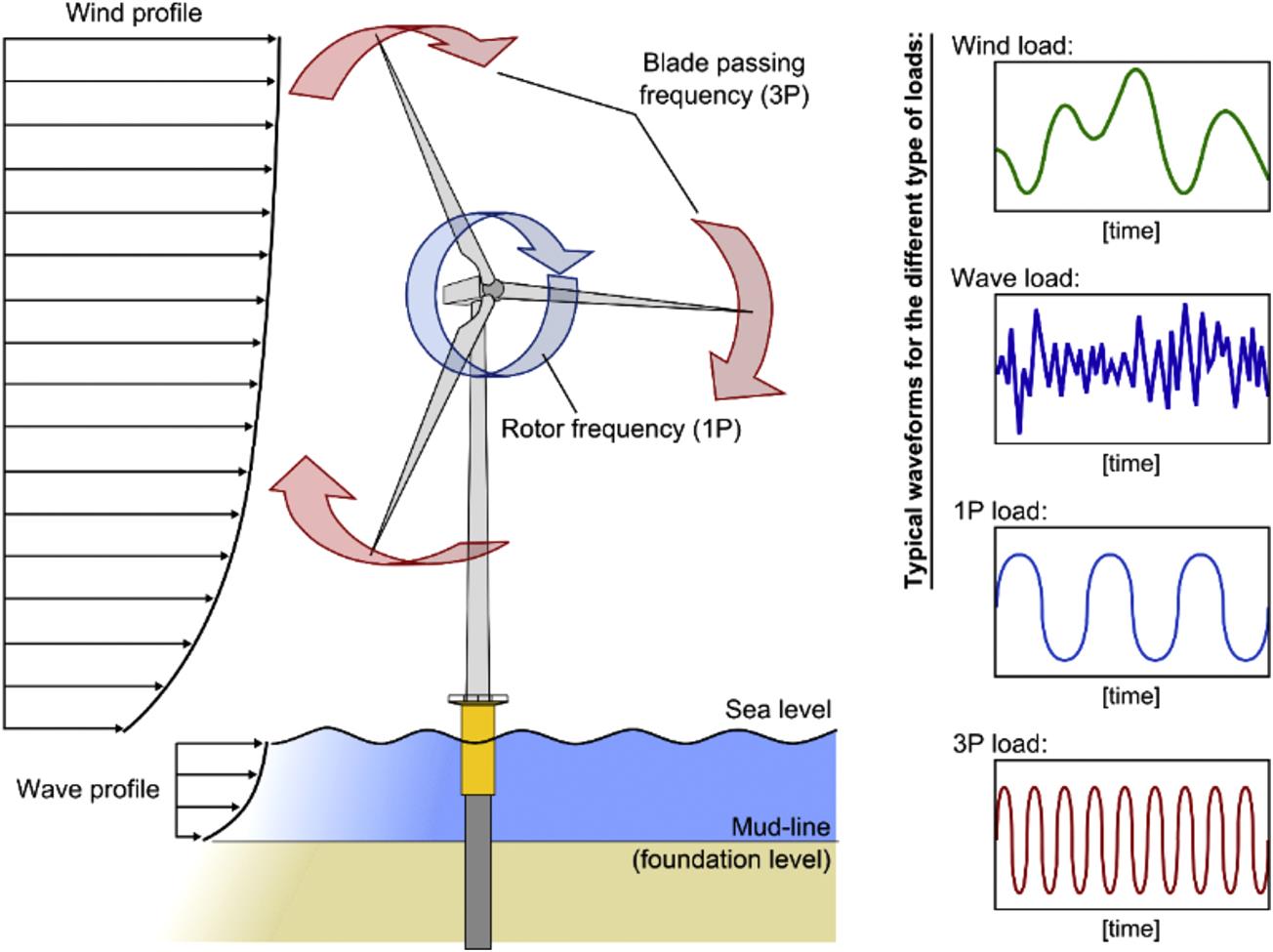

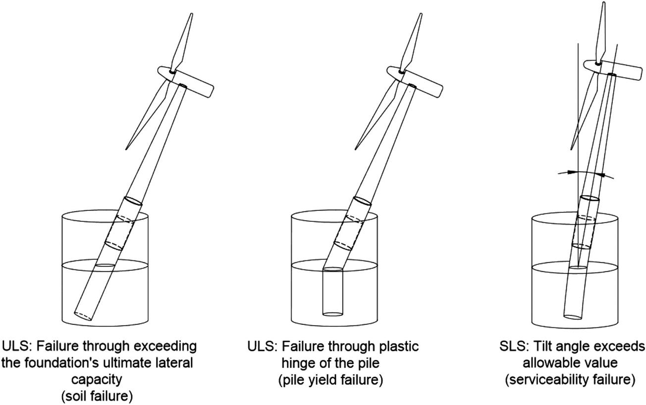
Fig. 14.3 describes schematically the mechanism to be considered at the design stage guided by Limit State Design philosophy. A commentary on the diagram is given further.
1. Ultimate Limit State (ULS): The first step in the design is to estimate the maximum loads on the foundations (predominantly overturning moment, lateral load and the vertical load) due to all possible design load cases and compare with the capacity of the chosen foundation. For monopile type of foundations, this would require computation of ultimate moment, lateral and axial load carrying capacity.
2. Target Natural Frequency (Eigen Frequency) and Serviceability Limit State (SLS): This requires the prediction of the natural frequency of the whole system (Eigen Frequency) and the deformation of the foundation at the mudline level (which can be further extrapolated to the hub level) over the lifetime of the wind turbine.
3. Fatigue Limit State (FLS) and long-term deformation: This would require predicting the fatigue life of the monopile as well as the effects of long-term cyclic loading on the foundation.
4. Robustness and ease of installation: This step will ascertain that the foundation can be installed and that there is adequate redundancy in the system.
One of the major uncertainties in the design of offshore wind turbines is the prediction of long-term performance of the foundation, i.e., the effect of millions of cycles of cyclic and dynamic loads on the foundation. The three main long-term design issues are:
1. Whether or not the foundation will tilt progressively under the combined action of millions of cycles of loads arising from the wind, wave, and 1P (rotor frequency) and 2P/3P (blade passing frequency). It must be mentioned that if the foundation tilts more than the allowable, it may be considered failed, based on SLS criteria and may also lose the warranty from the turbine manufacturer. The loads acting on the foundation are typically one-way cyclic and many of the loads are also dynamic in nature. Further details of the loading can be found in Arany et al. [1].
2. It is well known from literature that repeated cyclic or dynamic loads on a soil causes a change in the properties, which in turn can alter the stiffness of foundation, see Bhattacharya and Adhikari [2] and Bhattacharya [3]. A wind turbine structure derives its stiffness from the support stiffness (i.e., the foundation) and any change in natural frequency may lead to the shift from the design/target value and as a result the system may get closer to the forcing frequencies. This issue is particularly problematic for soft–stiff design (i.e., the natural or resonant frequency of the whole system is placed between upper bound of 1P and the lower bound of 3P) as any increase or decrease in natural frequency will impinge on the forcing frequencies and may lead to unplanned resonance. This may lead to loss of years of service, which is to be avoided.
3. Predicting the long-term behavior of the turbine taking into consideration wind and wave misalignment aspects [4,5].
The SLS and ULS modes of failure are schematically described in Fig. 14.3. ULS failure (which can also be described as collapse) can be of two types: (1) where the soil fails; (2) where the pile fails by forming a plastic hinge [6,7]. On the other hand, in SLS failure, the deformation will exceed the allowable limits. While the ULS calculations can be carried through standard methods, the SLS calculations and long-term issues requires detailed understanding of the Cyclic Soil–Structure Interaction as well as Dynamic Soil–Structure Interaction.
Fig. 14.4 shows a typical mudline bending moment acting on a wind turbine. Typically in shallow to medium deep waters, the wind thrust loading at the hub will produce the highest cyclic overturning moment at the mudline. However, the frequency of this loading is extremely low and is in the order of magnitude of 100 seconds (see Fig. 14.4). Typical period of wind turbine structures being in the range of about 3 seconds and therefore no resonance of structure due to wind turbulence is expected resulting in cyclic soil–structure interaction (SSI) [8,9].

On the other hand, the wave loading will also apply overturning moment at the mudline and the magnitude depends on water depth, significant wave height and the peak wave period. Typical wave periods will be in the order of 10 s (for North Sea) and will therefore have dynamic SSI. A calculation procedure was developed by Arany et al. [1] and the output of such a calculation will be relative wind and the wave loads; an example is shown in Fig. 14.4. It is assumed in the analysis that the wind and the wave are perfectly aligned which is a fair assumption for deeper water further offshore projects (i.e., fetch distance is high). Analysis carried out by Arany et al. [1] showed that the loads from 1P and 3P are orders of magnitude lower than wind and wave but they will have highest dynamic amplifications. The effect of dynamic amplifications due to 1P and 3P will be small amplitude vibrations. Resonance has been reported in operational wind farms in German North Sea, see Hu et al. [10]. Furthermore there are added SSIs due to many cycles of loading and the wind–wave misalignments. Typical estimates will suggest that offshore wind turbine foundations are subjected to 10–100 million load cycles of varying amplitudes over their lifetime (25–30 years). The load cycle amplitudes will be random/irregular and have broadband frequencies ranging several orders of magnitudes from about 0.001–1 Hz.
Based on the previous discussion, the SSI can be simplified into two superimposed cases and is discussed as follows:
1. Cyclic overturning moments (typical frequency of 0.01 Hz) due to lateral loads of the wind acting at the hub. This will be similar to a “fatigue type” problem for the soil and may lead to strain accumulation in the soil giving rise to progressive tilting. Due to wind and wave load misalignment, the problem can be biaxial. For example, under operating condition, for deeper water and further offshore sites, wind–wave misalignment will be limited for most practical scenarios. Wave loading, on the other hand, will be moderately dynamic as the frequencies of these loads are close to the natural frequency of the whole wind turbine system (typical wind turbine frequency is about 0.3 Hz).
2. Due to the proximity of the frequencies of 1P, 3P, wind, and wave loading to the natural frequency of the structure, resonance in the wind turbine system is expected and has been reported in German Wind farm projects [10,11]. This resonant dynamic bending moment will cause strain in the pile wall in the fore-aft direction, which will be eventually transferred to the soil next to it. This resonant type mechanism may lead to compaction of the soil in front and behind the pile (in the fore-aft direction).
Deformation of the pile under the action of the loading described in Fig. 14.4 will lead to 3-dimensional soil–pile interaction as shown schematically in Fig. 14.5. Simplistically there would be two main interactions: (1) due to pile bending (which is cyclic in nature) and the bending strain in the pile will transfer (through contact friction) strain in the soil, which will be cyclic in nature; (2) due to lateral deflection of the pile there will be strain developed in the soil around the pile. Fig. 14.5 shows a simple methodology to estimate the levels of strains in a soil for the two types of interactions and is given by Eqs. (14.1 and 14.2). The average strain in the soil at any section in a pile due to deflection can be estimated using Bouzid et al. [12] as follows:
(14.1)
where ![]() is the pile deflection at that section (for example A-A in Fig. 14.5) and DP is the pile diameter.
is the pile deflection at that section (for example A-A in Fig. 14.5) and DP is the pile diameter.

On the other hand, the shear strain in the soil next to the pile due to pile bending can be estimated using Eq. (14.2).
(14.2)
where M is the bending moment in the pile, I is the second moment of area of pile, and EP is the Young’s Modulus of the pile material. It must be mentioned that Eq. (14.2) assumes that 100% of the strain is transmitted to the soil, which is a conservative assumption and calls for further study. In practice this will be limited to the friction between the pile and the soil.
14.1.1 Need for Numerical Analysis for Carrying out the Design
The previous section showed a simplified procedure to estimate SSI. However, this approach is grossly oversimplified and has limitations in the sense that the changes in soil properties due to cyclic loading cannot be considered. Also whether or not the foundation will progressive tilt cannot be studied. While the two simple interaction phenomena (i.e., due to pile bending and to lateral deflection of the pile) are taken into consideration, other aspects, such as interface opening (gap formation) or possible impacts between pile and soils during the dynamic loading cannot be accounted for. Moreover, the nature of dynamic loadings is complicated due to the wind–wave misalignment. These considerations make it necessary to use numerical simulations, which allow one to precisely define the geometry of the problem and can also encompass different types of soils. Furthermore changes in the behavior of the soils surrounding the pile is expected to occur as a consequence of the repetition of cycles. Advanced constitutive models, suitable to reproduce different aspects of cyclic/dynamic behavior, are therefore required for analysis. Classical elastoplastic models cannot estimate the accumulation of plastic volumetric strains due to the repetition of cycles (densification). Therefore advanced constitutive laws capable of simulating the plastic strains in soils not due to the magnitude of the loading, but due to the repetition of cycles are needed [13–15].
14.2 Types of Numerical Analysis
Different types of numerical analysis ranging from very simple and practical to more theoretical and standardized can be carried out depending on the application. The methods can be classified into three groups: (1) Simplified where closed form solutions are used and useful during the conceptual and financial feasibility stage; (2) Standard method where code-based calculations are carried out. In the context of monopile, the standard analysis is the p–y analysis (nonlinear Beam on Winkler Foundations), Winkler [16]; (3) Advanced analysis that requires specialist knowledge and expertise. In the detailed design stage, advanced analysis is necessary to predict the long-term prediction. The aim of this chapter is to present advanced numerical models that are suitable to model the SSI [17].
14.2.1 Standard Method Based on Beam on Nonlinear Winkler Spring
The American Petroleum Institute (API) code prescribes a methodology known as “p–y” method, which is widely used for design of offshore piles. This is a subgrade modulus method with nonlinear depth dependent load—deformation characteristics representing the pile–soil interaction. This procedure is calibrated to provide the worst case scenario for the foundation behavior under static and cyclic loading. The p–y curve has been adopted in most offshore standards (like API, 2007; GL, 2005; DNV, 2004 or ISO,) as it has been considered, for many years, as the best method available to determine the displacements of the head of the pile under various loading conditions. Fig. 14.6 represents a typical p–y curve and in the figure, from a to b, an increase in the loading carries an increasing rate of degradation. This nonlinear behavior can be determined empirically or using field tests, under either static or monotonic loading conditions. On the other hand, Fig. 14.6B shows the degradation suffered by the soil as the pile deflection increases [19,20,21].
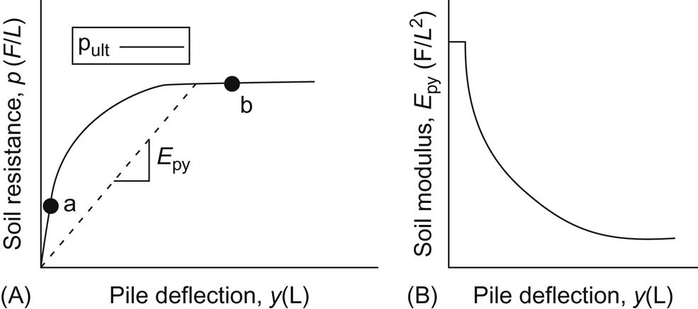
Terzaghi [22] demonstrated that the linear relationship between p and y (from the origin to a in Fig. 14.6A) was only valid for values of p lower than a half of the ultimate bearing capacity of the soil [22]. This criteria is assumed in the construction of the p–y curves by many methodologies. API (2007) [23] takes into account a number of factors for the construction of the curves, which can be summarized as follows:
Some other aspects, such as the effects of pile installations in the soils and the scour, are taken into account, although it is fully recognized that these factors require further analysis and research.
The main limitations of this API (2007) are:
1. The p–y curve is a procedure verified for piles up to 2 m diameter [19] and this is one of the main limitations of this methodology, as the monopiles in OWT currently have diameters of around 6 m. Extrapolation of a calibrated method is not advisable in geotechnical engineering. Achmus and Abdel-Rahman [19] demonstrated that p–y curve underestimates the deflections of piles, compare to some numerical simulations. Other researches also demonstrate that p–y curve overestimates the pile–soil stiffness for large diameter piles [24].
2. The nonlinear behavior expected for very high loads in large diameter piles are not covered by this methodology, because the calculated displacements are small if related to the pile diameter (although they can be very big in absolute terms) [19].
3. When the piles are installed in layered soil, the material is taken as continuous and the interaction between the different layers is neglected. This limitation does not occur when the curves are derived on the basis of full-scale tests [18].
4. The subgrade reaction coefficient, k, does not contain any effect related to the flexural stiffness of the pile or the type of loading.
Computational simulations are the alternative to overcome those limitations. Different trends in these methodologies and few worked out examples are presented next, in order to address their suitability and reliability.
14.2.2 Advanced Analysis (Finite Element Analysis and Discrete Element Modeling) to Study Foundation–Soil Interaction
14.2.2.1 Different Soil Models Used in Finite Element Analysis
To account for accumulated strains in the numerical simulations, it is necessary to employ a suitable constitutive model, capable of reproducing realistic soil behavior when subjected to cyclic/dynamic loading conditions. Simple elastoplastic models are usually based on one yield surface without hardening (e.g., the Mohr Coulomb model), with isotropic hardening (e.g., the Cam-Clay model), or on two yield surfaces (isotropic loading and deviatoric loading), e.g., Lade’s. They are ideal and efficient on simulating the soil behavior under monotonic conditions, but not suitable to model cyclic loading. Essentially, in such models, plastic deformations start to appear for a certain magnitude of loading, usually higher that the amplitude of the cycles, and hence, the simulated soil behavior remains elastic under that limit, which is against experimental evidences particularly for granular soils [25]. Fig. 14.7 shows the different phenomenon, which can take place in soil during cyclic loading.
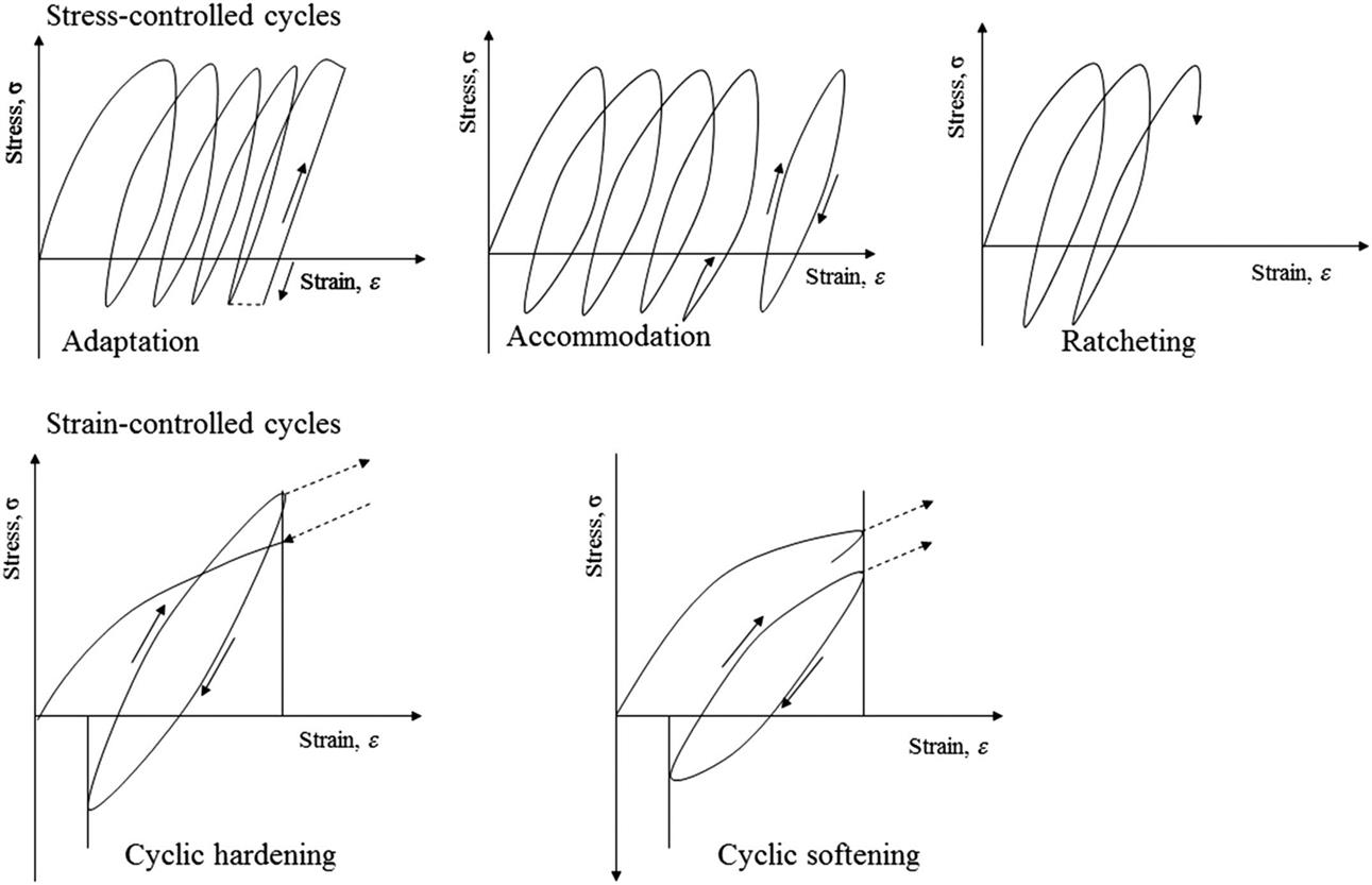
Plastic phenomenon for cyclic loading can either be based on “constant stress amplitude” (so called stress controlled) or “constant strain amplitude” (strain controlled). The phenomenon called “adaptation” refers to less dissipation of energy in each cycle of loading as the number of cycles increases, until convergence to nondissipative elastic cycles. On the other hand “accommodation” refers to change of the dissipation of energy from the beginning with an irreversible cumulative deformation and evolves toward a stabilized cycle. This is experienced in laboratory experiments for drained samples. “Ratcheting” is an irreversible strain accumulation, which keeps the same shape as that of the beginning [25].
Constant strain amplitude cyclic loading phenomenon results in the cyclic hardening or softening. Cyclic hardening occurs when there is an increase in the cyclic stress amplitude with an increase in the number of cycles, e.g., densification during testing of drained soil. On the contrary, cyclic softening occurs when there is a reduction in the cyclic stress amplitude as the number of cycles increases, e.g., an increase in pore pressure during the testing of undrained soil samples (decrease in the effective stress).
In one of the examples presented in this chapter, a kinematic hardening law has been employed by coupling the elastic moduli and a hardening parameter. Kinematic hardening is used to model plastic ratcheting, which is the build-up of plastic strain during cyclic loading, as previously explained. Other hardening behaviors include changes in the shape of the yield surface in which the hardening rule affects only a local region of the yield surface, and softening behavior in which the yield stress decreases with plastic loading. The kinematic hardening model only involves one plastic mechanism with a smooth yield surface. For nonlinear modeling, the material behavior is characterized by an initial elastic response, followed by plastic deformation and unloading from the plastic state. The plasticity is as a result of the microscopic nature of the material particles and includes shear loading that causes particles to move past one another, changes in void or fluid content that result in volumetric plasticity, and exceeding the cohesive forces between the particles or aggregates. The material is defined by model materials subject to loading beyond their elastic limit. See Refs. [25,26] for more details.
14.2.2.2 Discrete Element Model Analysis Basics
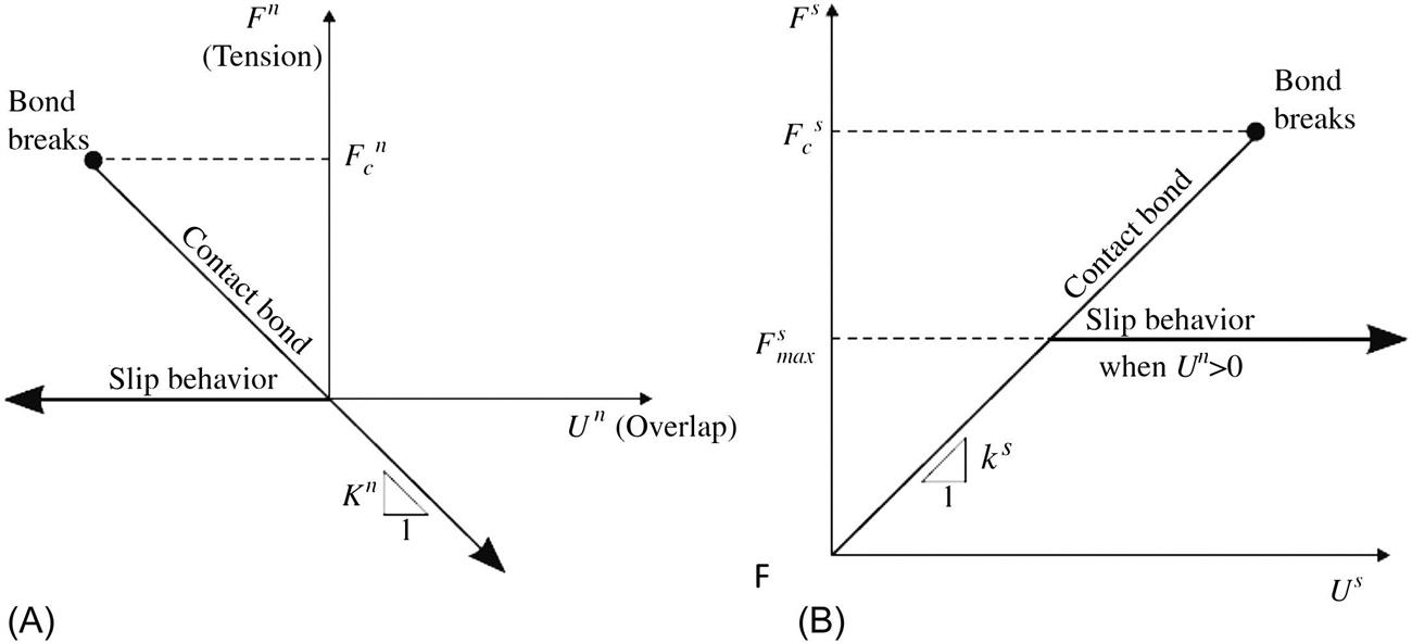
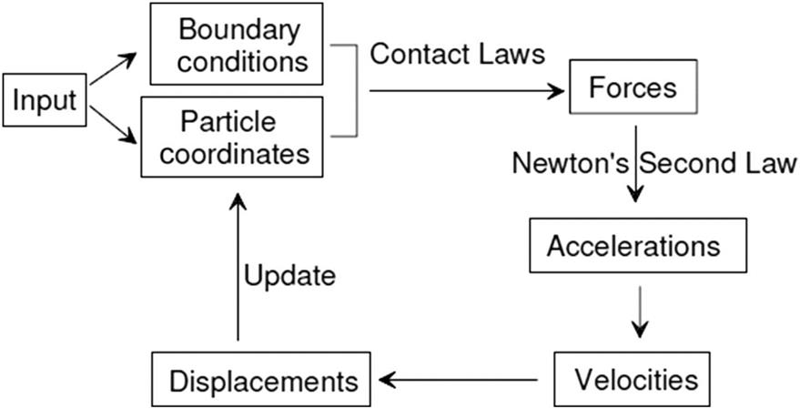
Originally proposed by Cundall and Strack [26], Discrete Element Method (DEM) simulates granular materials as assemblies of individual particles, which respond to given load conditions. The interactions between particles are simulated by contact laws, e.g., linear contact model, Hertz-Mindlin contact model [27], and parallel bond model, where the normal and tangential contact forces are dependent on the overlap and relative displacement between two contact particles (Fig. 14.8). The contact forces, accelerations, velocities, and displacements of all particles are updated in each small time step using the central difference time integration method. Stresses and strains are then calculated from the contact forces within a representative volume element (RVE) or along a boundary. The DEM is superior to other numerical methods (e.g., Finite Element Method (FEM)) as it allows the direct monitoring of change in soil stiffness, and more importantly it offers a method to analyze the micromechanics, which underlies the stiffness changes. Fig. 14.9 shows a flowchart of a typical DEM calculation.
14.3 Example Application of Numerical Analysis to Study SSI of Monopile
This section of the chapter shows different applications of numerical analysis to investigate phenomenon related to long-term performance as explained in Section 14.1.
14.3.1 Monopile Analysis Using DEM
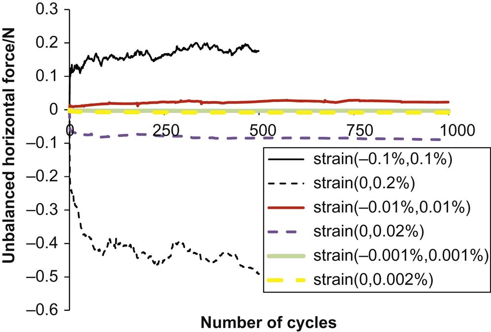
An analysis of monopile–soil interactions and stiffness variations were carried out using an open-sourced DEM code modified and validated in previous studies (Cui [29], Cui et al. [30], O’Sullivan et al. [31]). More details can be found in Cui and Bhattacharya [32]. A DEM model of a soil tank (100 mm×100 mm×50 mm) was firstly created, which was filled with about 13 000 spherical particles of radii in the range of 1.1–2.2 mm. The particles were deposited under gravity. The pile was 20 mm in diameter and was embedded to a depth of 40 mm by removing particles located in the space, which was to be occupied by the pile. Particles were allowed to settle down again following the installation of the pile. Once the soil particles were settled down in the soil tank, cyclically horizontal movements were assigned to the pile to simulate the cyclic movements of OWT monopile due to the cyclic loadings. Translational movements rather than rotational movements were assigned to the pile at this stage. Three different strain amplitudes, 0.1%, 0.01%, and 0.001%, were chosen to examine the effects of strain levels. For each strain amplitude two types of cyclic loading were applied: symmetric cyclic loading with stains in the ranges of (−0.1%, 0.1%), (−0.01%, 0.01%), and (−0.001%, 0.001%) and asymmetric cyclic loading with strains in the ranges of (0, 0.2%), (0, 0.02%), and (0, 0.002%). As constrained by the computational costs, 500 cycles were simulated for strain amplitude of 0.1% and 1000 cycles were simulated for other strain amplitudes. The simulation parameters are listed in Table 14.1.
Table 14.1
Input Parameters for Discrete Element Method (DEM) Simulation
| Parameters | Value |
| Soil particle density ρs/kg m−3 | 2650 |
| Particle sizes/mm | 1.1, 1.376, 1.651, 1.926, 2.2 |
| Interparticle frictional coefficient (μ) | 0.3 |
| Particle-boundary frictional coefficient (μ) | 0.1 |
| Gs (Hertz-Mindlin contact model) (Pa) | 2.868×10⁷ |
| Poisson’s ratio | 0.22 |
| Initial void ratio/e | 0.539 |
The resultant horizontal stress applied on the pile versus the horizontal strain of soil is illustrated in Fig. 14.10. It can be observed that the stress–strain curves forms hysteresis loops, indicating the energy dissipations during the cyclic loading. It is also interesting to observe that, though the stresses in the first half cycle for the asymmetric cyclic loading is positive, it reduced to negative when the strain goes to zero. Following a few cycles, the minimum negative stress approaches the same magnitude as the maximum positive stress. Moreover the magnitude of stresses and the shape of the hysteresis loops for both symmetric cyclic loading and asymmetric cyclic loading are almost identical after many cycles. The system under asymmetric cyclic loading behaves the same as symmetric cyclic loading with the same strain amplitude after many cycles, indicating that the strain amplitude, rather than the maximum strain, dominates the long-term cyclic behavior.

The secant Young’s Modulus of soil in each cycle was calculated by determining the slope of a line connecting the maximum and minimum points of each full loop and is shown in Fig. 14.11. It is evident that the secant Young’s Modulus of soil increased during the cyclic loading. The initial stiffness of asymmetric cyclic loading is lower than that of symmetric cyclic loading with the same strain amplitude due to higher maximum strain applied. However, following a few cycles, the stiffness for both types of cyclic loading approaches the same value. The Young’s Modulus versus horizontal strain in the first half cycle and in the 500th cycle for strain amplitude of 0.1% is shown in Fig. 14.12. The stiffness–strain curve in the first cycle displays the similar “S” shape as expected for the shear modulus–shear strain curve. Following cyclic loadings, all stiffness at different strain levels increases significantly.


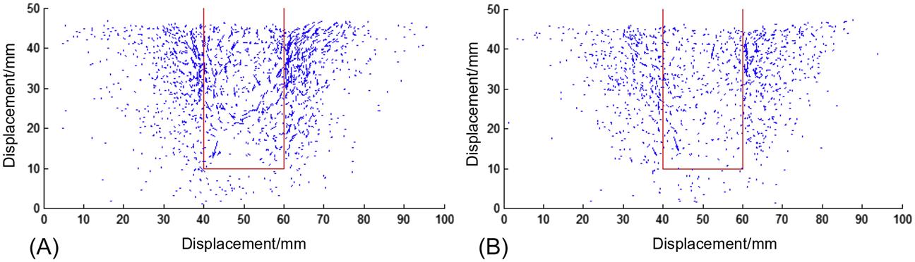
To illustrate the ground settlement, plots of incremental soil particle displacements in the symmetric cyclic loading with strain amplitude of 0.1% in the first 50 cycles and in the next 50 cycles are given in Fig. 14.13. Each arrow in the plot starts from the original center of a particle and ends at the new center at the end of a given cycle. It is evident that soil particles surrounding the pile moved downwards, causing ground settlement. Soil densification around pile is the main reason causing the increase of soil stiffness. It also clear that the soil particle displacements are only significant in the first 50 cycles, underlying the significant increase in the soil stiffness in the first 50 cycles. In the current DEM simulations samples with same initial void ratio of 0.539 (medium dense sample) all showed densification behavior and stiffness increase under cyclic loading. It would be interesting to investigate soil behaviors and stiffness evolutions for a wide range of initial void ratios in the future study.
The evolutions of average radial stress in representative cycles are illustrated in Fig. 14.14. Due to the soil densification, the radial stress increased significantly for strain amplitude of 0.1% under cyclic loading. The shapes of the radial stress–strain curves are quite different for different strain amplitude. For symmetric cyclic loading with 0.01% strain amplitude (Fig. 14.14C), the radial stress increases at positive strain values, but decreases slightly at negative strain values. However, for 0.1% strain amplitude (Fig. 14.14A), the radial stress increases at both positive and negative strains, forming a “butterfly” shaped curve. It is also interesting to observe that, for the asymmetric cyclic loading (Fig. 14.14B), the stress–strain response in the first few cycles is different from that in the correlated symmetric cyclic loading, However, it eventually evolves to the same “butterfly” shape after many cycles. It confirms again that the influence of different maximum strain of a cyclic loading can be eliminated after many cycles and the dominant factor for cyclic soil response is strain amplitude.

The evolution of unbalanced horizontal force at the end of each cycle is illustrated in Fig. 14.15. It is evident that the unbalanced horizontal force is more significant with increasing strain amplitude. It can also be seen that the unbalanced force for asymmetric cyclic loading is much larger in magnitude and is oriented in the opposite direction compared with that for symmetric cyclic loading. It is because, for asymmetric cyclic loading pile only moves to the right side and compresses the soils on the right side significantly, therefore the horizontal force on the pile at the end of each cycle is oriented to the left. However, for the symmetric cyclic loading, the pile compressed the soils on both sides to the same strain level. At the end of a full cycle, the residual horizontal force is oriented to the right. In the presented study monopile was driven to move by a predefined constant velocity. It is more realistic to simulate the free motions of monopile under the action of resultant external force/moment, including the interaction force/pressure between the monopile and the soil.
14.3.2 Monopile Analysis Using FEM Using ANSYS Software
This section of the chapter presents the analysis of a monopile embedded 30 m in a cylindrical soil layer (90 m wide, 45 m deep), see Fig. 14.16. The steel pile is open ended with a wall thickness of 90 mm and a diameter of 7.5 m. It is worth noting that monopile diameters of up to 7 m are designed to maintain serviceability of the wind energy converters over several years as a result of harsh environmental conditions offshore. The monopile extended 30 m above the sea bed to the point where it was loaded and driven 30 m into the sea bed where the water depth was 10 m. The software ANSYS 17.0 was used to create the 3D model of wind turbine foundation. Static Structural Analysis was used to analyze static conditions, while the Transient Structural was used for the cyclic load.
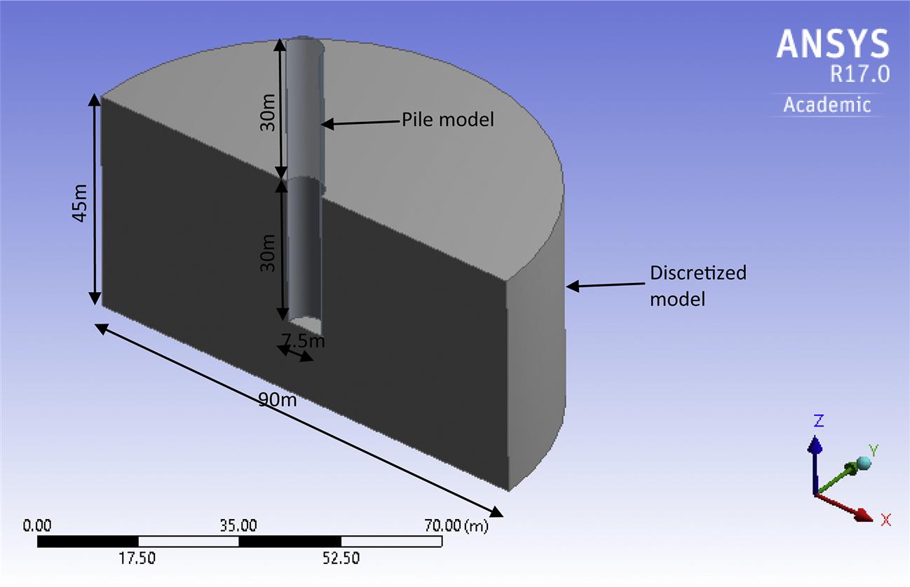
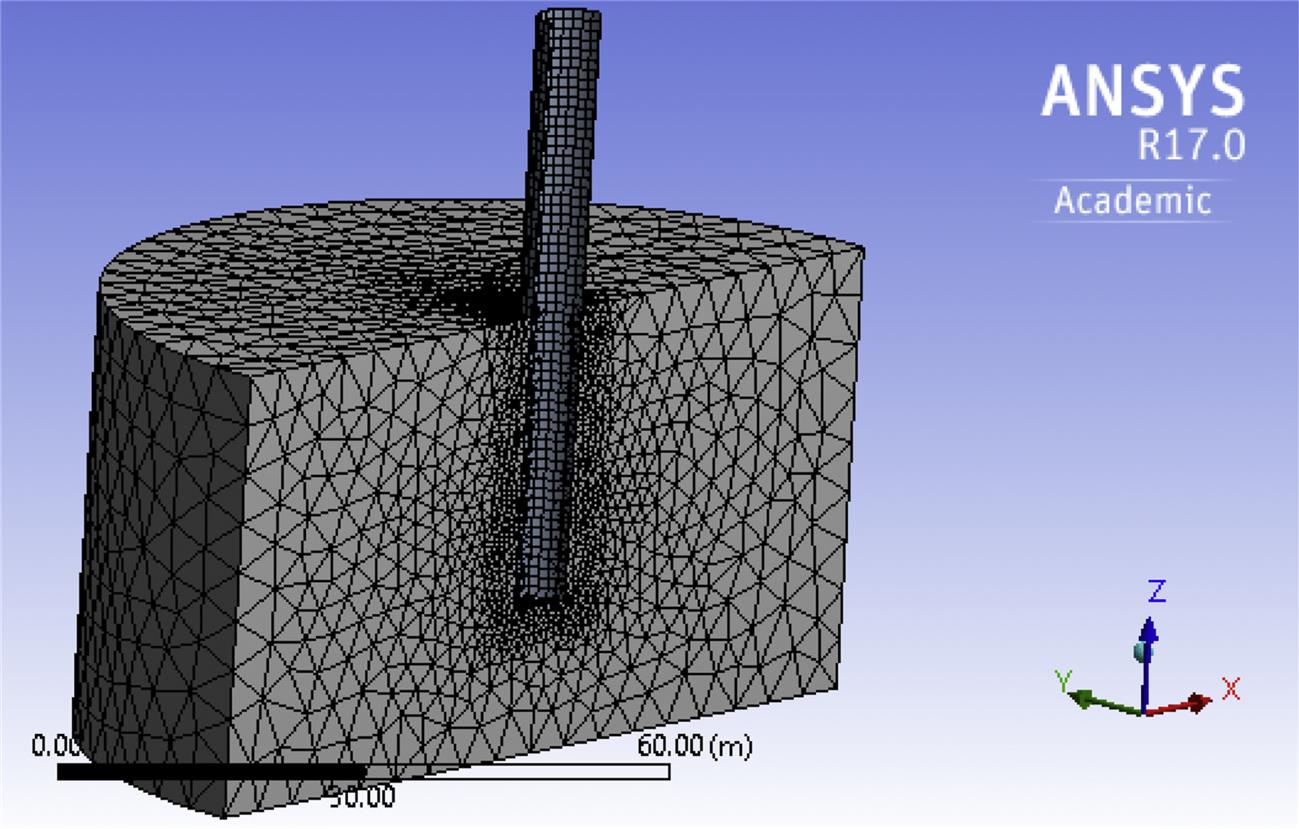
The soil–pile model took advantage of the symmetry in geometry and load, hence, only one half of the soil-pile model was modeled, as shown in Fig. 14.17 which means that the transversal displacements at the symmetry plane was set to zero. A fine mesh size was selected for the system as shown in Fig. 14.17 resulting in 50 622 nodes and 36 816 elements. Previous studies demonstrated that the minimum number of elements required for an accurate enough model of monopile wind turbine foundations may be in the range of 30 000–40 000. The interaction between pile and structure was modeled as a frictional interface with friction coefficient of 0.4.
The time step was taken as 0.5 second, which was derived by the integration time step (ITS) method [33]. The force was applied by an idealized system described by Bryne and Houlsby [34] with a generalized loading case for a 3.5 MW turbine in which a 4 MN horizontal load and a 6 MN vertical load applied 30 m above the soil surface was used. This can be represented as:
(14.3)
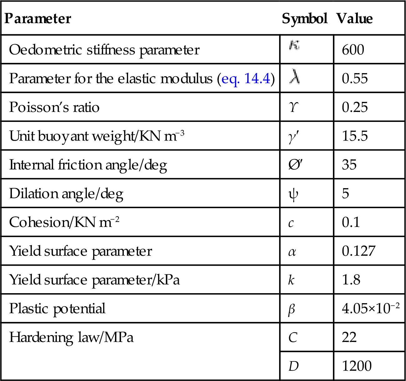
The one-way lateral load was applied with a sinusoidal character of 0.1 Hz (typical frequency ranges in these infrastructures are 0–1 Hz for environmental loads and 5–200 Hz for machine loads [34]). At fixed end time, t of 1000 seconds was used, this gave 100 cycles (frequency=0.1 Hz), which was used in analyzing the results. The input parameters for the pile were calibrated for offshore installation in United Kingdom using typical test results while those obtained after calibration for the soil are shown in Table 14.2. The steel monopile was represented as a linear-elastic, isotropic, homogeneous material. For the soil properties, the Kinematic Hardening law, have been employed.
Table 14.2
Soil Model Material Parameters for Medium Dense Sand (after [19])
| Parameter | Symbol | Value |
| Oedometric stiffness parameter | 600 | |
| Parameter for the elastic modulus (eq. 14.4) | 0.55 | |
| Poisson’s ratio | Υ | 0.25 |
| Unit buoyant weight/KN m−3 | γ′ | 15.5 |
| Internal friction angle/deg | Ø′ | 35 |
| Dilation angle/deg | ψ | 5 |
| Cohesion/KN m−2 | c | 0.1 |
| Yield surface parameter | α | 0.127 |
| Yield surface parameter/kPa | k | 1.8 |
| Plastic potential | β | 4.05×10⁻² |
| Hardening law/MPa | C | 22 |
| D | 1200 |
The elastic modulus of the soil was derived from Janbu (1963) as presented in Eq. (14.2):
(14.4)
where ![]() denotes the soil vertical effective stress, and
denotes the soil vertical effective stress, and ![]() is the atmospheric pressure.
is the atmospheric pressure.
The plot of the applied horizontal load versus the pile-head displacement for dynamic loading, p–y (Fig. 14.18) shows a progressive inclination of the hysteretic loops, for every subsequent increase in the number of cycles, resulting in an increasing pile-head displacement. Similar trend can be observed in the result reported in Ref. [13], although that analysis was carried out for a clayey soil under the influence of a two-way lateral loading, which resulted in equal but opposite pile displacements in both directions. This result trend can be referred to as accommodation cyclic behavior (previously presented in this chapter) and is mostly found in laboratory experiments [25].
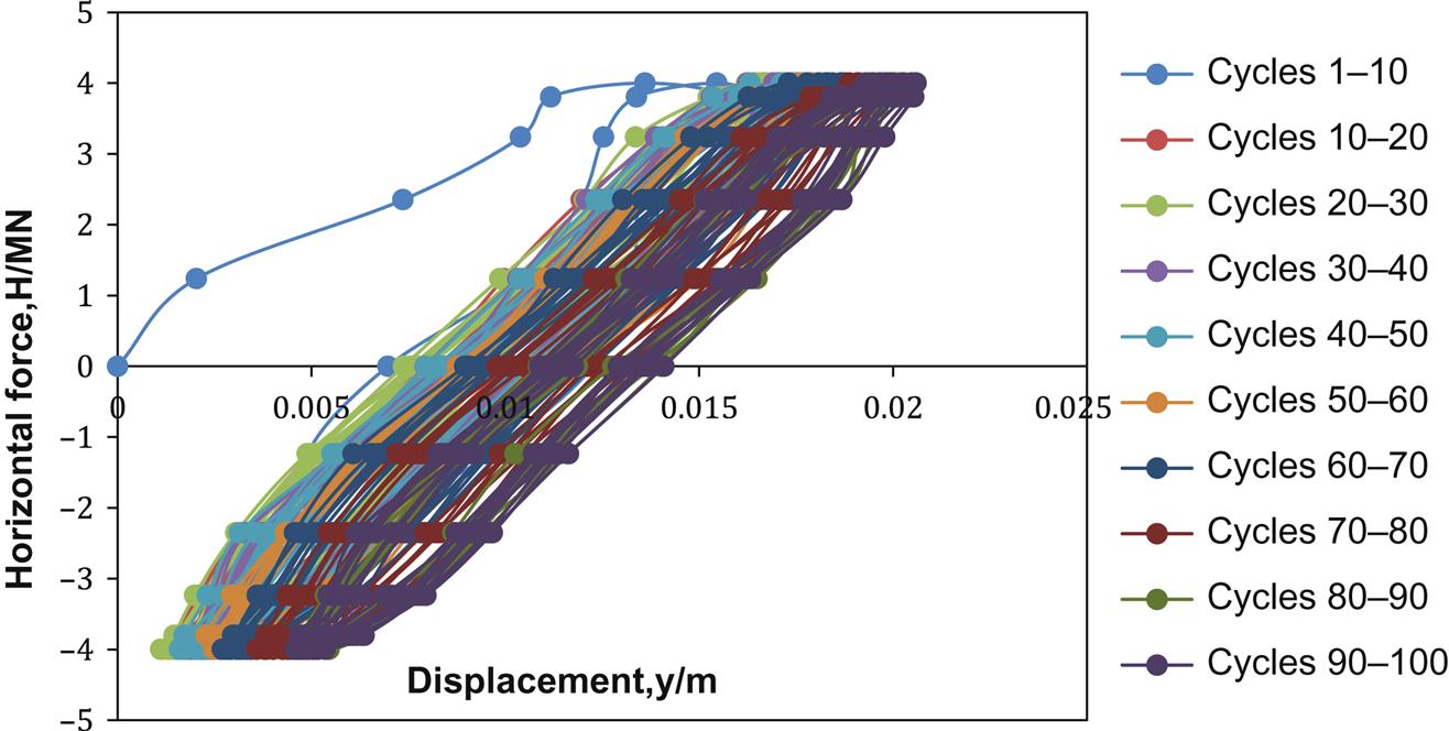
A closer observation of pile-head displacement (Fig. 14.19) shows an increase in the displacement with time. This can be observed in drained cyclic tests with an increase in density (densification) [25]. However, instabilities caused by alternating degradation and compaction are observed at the earlier cycles, causing negative displacement accumulation at the initial stages of loading. The pile-head displacement at the end of the first cycle equals 1.36 cm and 2.06 cm at the end of 100 cycles, which is the maximum displacement of the sea bed in front of the pile. This gives a total increased displacement of 0.7 cm. The accumulation rate from the 1st to the 100th cycle equals 1.51 cm. The displacement accumulation per cycle reduces drastically for the first 10 cycles, and then tends toward zero as the number of cycles increase, because at deflections larger than that of static loading, the value of soil resistance, p, decreases sharply due to cyclic loading, while afterwards it remains pretty much constant [18]. This is as a result of the kinematic hardening parameter, as also reported in Ref. [25], which stated that the cycles become reversible until a complete stabilization is reached for very high numbers of cycles. Similar results are observed along radial stress paths [35,36].

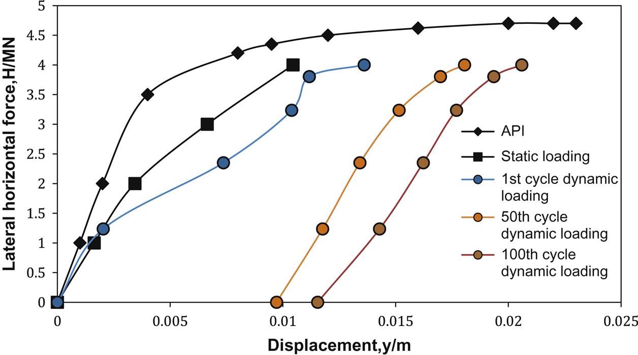
A comparison of the load-displacement response at the pile head between results from finite element modeling (static and dynamic) and API p–y curve method is provided in Fig. 14.20. The dynamic loading is represented by the curve for 1st, 50th, and 100th cycle. From Fig. 14.20, it is observed that at very low lateral-horizontal forces, the API method is in agreement with numerical simulations for static loading and 1st cycle dynamic loading. This supports the statement that the API method is a pseudo static approach [18]. However, at low lateral-horizontal forces and high number of cycles, the API method underestimates the pile displacement. This can be observed by the difference in pile displacements between the API method and numerical simulations; calling Δ to the displacement obtained when the applied load is 4 MN, we can see that Δ equals 0.3 cm for the 1st cycle, 0.8 cm for the 50th cycle, and 1 cm for the 100th cycle. This underestimation of the pile displacement by the API method at low lateral displacement was also observed by Hearn [37]. This also represents the conclusion presented by Yang et al. [38] who stated that “the cyclic bearing capacity may be significantly lower than the static bearing capacity.” This is true as the displacement increases with an increase in the number of cycles. Thus the displacement as a result of several cycles goes farther away from the displacement from static load/one cycle, since there is an accumulation of volumetric strains in the soil surrounding the pile. The plot also shows that the curve for the static loading and the 1st cycle dynamic loading are similar but the difference in pile displacement at the maximum applied lateral load of 4 MN is 0.3 cm. This gives a percentage difference of 30%. This may be because simulations for transient analysis are based on division of time or steps: therefore, there is a progressive accumulation of residual errors with an increase in the number of time steps [39].