CHAPTER |
4 |
CASE STUDIES
4.1 Introduction
In the preceding chapter, we discussed the baseline model or perfect scenario in which the project is neither early nor late and is completed on budget. To carry our study forward, we will develop alternative simulations for the same project and compare these with the baseline project in order to make observations and derive conclusions.
For the purpose of this study, we will consider two alternatives:
- Finishing ahead of schedule (early completion) because of efficient utilization of resources
- Finishing behind schedule (delayed completion) as a result of mismanagement and slackness
4.2 Alternative 1: Early Completion Simulation
In this scenario, the project manager has taken an efficient, engineering approach to plan and execute the project.
Some distinct factors of this scenario include the following:
- Through proper use of project management tools and techniques, thorough and proper planning was done for the sequence of activities and the estimation of resources and durations.
- Consideration was made for the use of advanced equipment and machinery supplied on time and in the required quantities during the execution phase, thus reducing activity durations.
- Skilled laborers capable of “planning their work and then working their plan efficiently” were procured in the required quantities. As a result, activity durations were reduced because the work was being done more efficiently.
- Critical path analysis, fast tracking, and crashing of critical activities of the schedule through the utilization of additional manpower and resources also resulted in additional costs. However, the impact of these additional costs does not make Alternative 1 go over budget as these amounts were spent to increase the efficiency of work done and reduce activity durations as a trade-off.
4.2.1 Alternative 1 Project Schedule
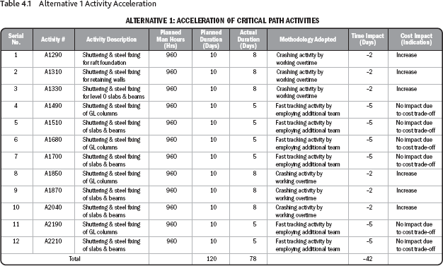
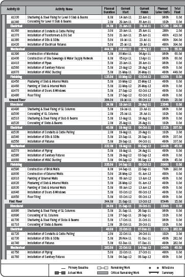
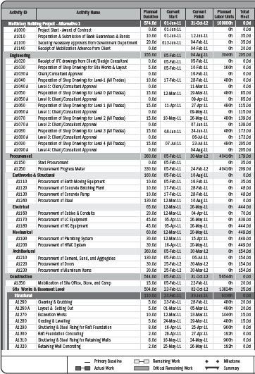
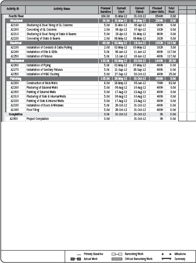
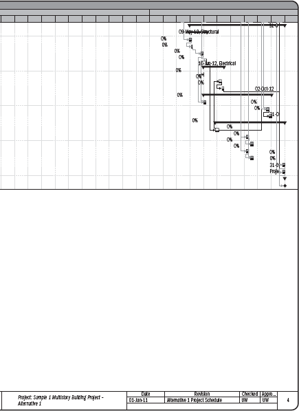
The above approach affected the following activities and resulted in an overall acceleration of the project's schedule. Table 4.1 also indicates the cost effect of these activities, which is used for further study in this research.
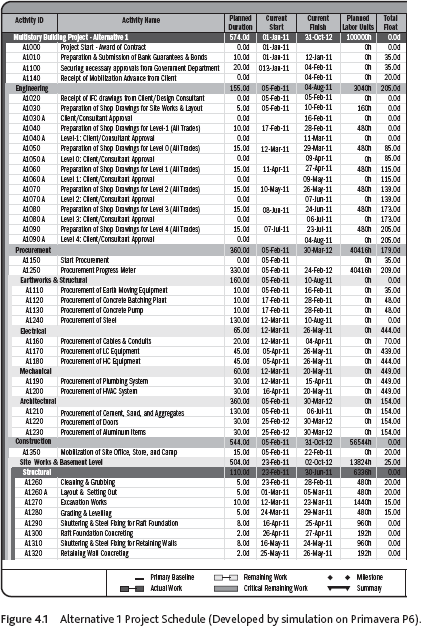
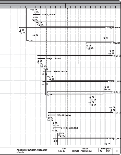
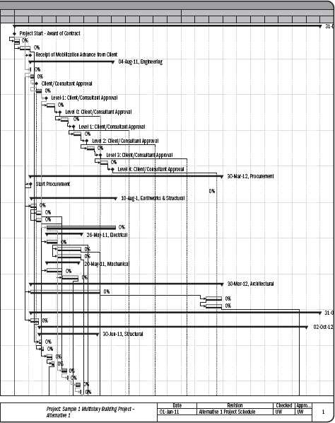
Figure 4.1 portrays the schedule prepared on P6 for the same project but simulated to complete early as an outcome of the above factors.

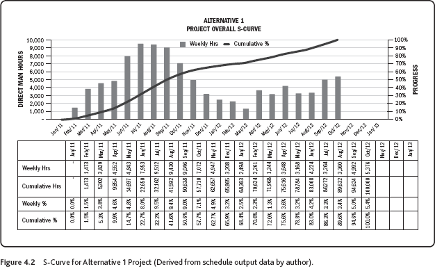
4.2.2 Alternative 1 Project S-Curve
Using output from the developed Primavera file for weekly and cumulative man hours, the S-curve shown in Figure 4.2 has been developed for Alternative 1.
4.2.3 Cost/Earned Value Management of Alternative 1
Original Budget = 363,014,661
At the 25% stage of the project:
Planned Value (PV) = 90,753,665
Earned Value (EV) = 90,753,665 (indicating 25% project completion)
Actual Cost (AC) = 110,900,000
Schedule Performance Index (SPI) = EV/PV = 1.00 (on schedule)
Cost Performance Index (CPI) = EV/AC = 0.81 (over budget)
Forecasted Estimate at Completion calculated at this stage = BAC/CPI = 448,166,248
At the 50% stage of the project:
Planned Value (PV) = 181,507,330
Earned Value (EV) = 217,808,796 (indicating 60% project completion)
Actual Cost (AC) = 225,000,000
Schedule Performance Index (SPI) = EV/PV = 1.20 (ahead of schedule)
Cost Performance Index (CPI) = EV/AC = 0.96 (over budget)
Forecasted Estimate at Completion calculated at this stage = BAC/CPI = 378,140,271
At the 75% stage of the project:
Planned Value (PV) = 272,260,995
Earned Value (EV) = 308,562,461(indicating 85% project completion)
Actual Cost (AC) = 308,562,461
Schedule Performance Index (SPI) = EV/PV = 1.13 (ahead of schedule)
Cost Performance Index (CPI) = EV/AC = 1.00 (on budget)
Forecasted Estimate at Completion calculated at this stage = BAC/CPI = 363,014,661
At the 100% stage of the project:
Planned Value (PV) = Budget at Completion (BAC) = 363,014,661
Earned Value (EV) = 363,014,661
Actual Cost (AC) = 363,014,661
Schedule Performance Index (SPI) = EV/PV = 1.00 (an obvious expectation because, in terms of value, the project is complete even if it is completed ahead of time)
Cost Performance Index (CPI) = EV/AC = 1.00
4.2.4 Observations
From these data, we can see that Alternative 1 results in the following:
- The project is completed 2 months before the deadline, on October 31, 2012.
- The project is completed at the budgeted cost because additional resources for fast tracking and crashing the schedule allow overheads and indirect costs associated with duration to be reduced.
- It is pertinent to mention here that according to Section 3.1 of this study, the contract is a fixed price with incentive type, and an incentive of 0.1% of contract price per day earlier completed was permissible on this contract up to a maximum of 10% of the contract price. Thus, the value of the incentive that the project earned was:
Bonus for 60 days = 0.1% of 363,014,661 × 60 = 21,780,879
Thus, the net actual value of the project is:
Revised Actual Cost = 363,014,661 – 21,780,879 = 341,233,782
(That is, the project has a profit of 21,780,879.)
Revised CPI at completion = 1.06 (the project is completed under budget)
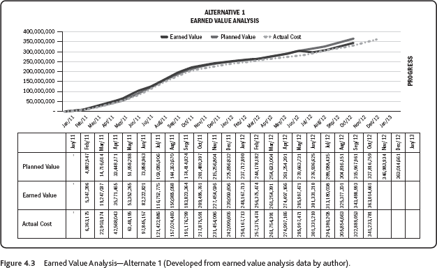
The Earned Value Analysis for the Alternative 1 project simulation is shown in Figure 4.3.
4.3 Alternative 2: Delayed Completion Simulation
In this undesirable scenario, the project manager has taken an inefficient, non-engineering approach to plan and execute the project, which has become a problematic situation.
Below are some distinct factors of this scenario:
- Proper use of project management tools and techniques was not made, and the project was not thoroughly planned.
- The project did not utilize modern technology and equipment to perform the work more efficiently.
- On various occasions, the project faced a shortage of materials because of improper planning of procurement and bad reporting from the site.
- The workload was not properly planned, which led to a waste of resources and idle hours, thus losing productivity and causing delays. This factor led to increased activity durations.
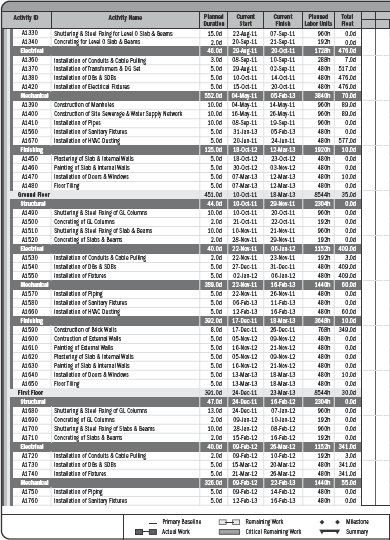
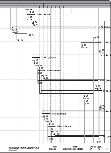
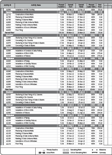
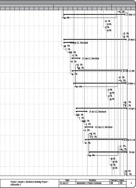
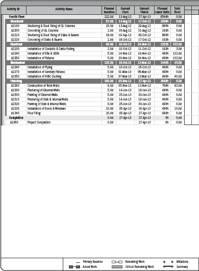
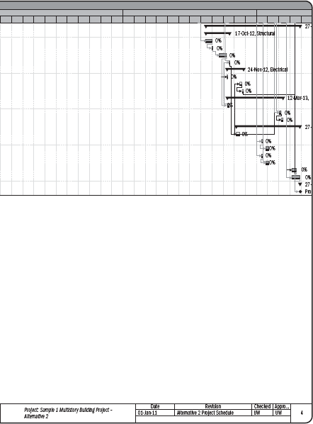
4.3.1 Project Schedule
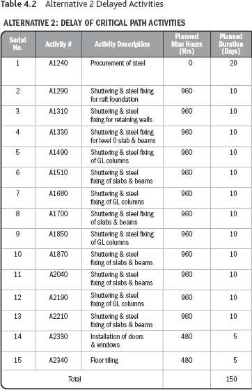
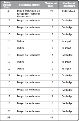
The activities shown in Table 4.2 were affected as a result of the above approach, resulting in an overall delay of the schedule. Their cost effect is also indicated. It is used for further study in this research.
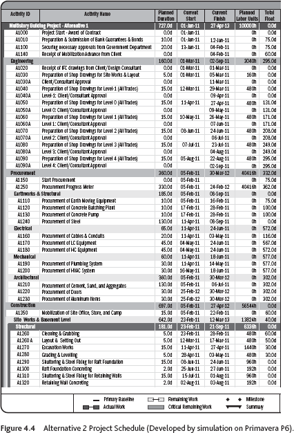
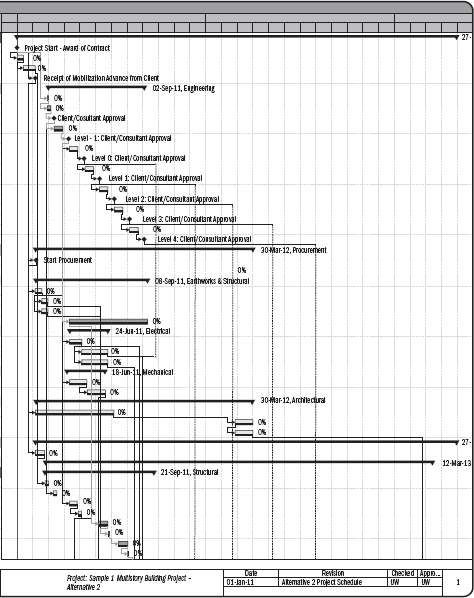
The project was simulated on Primavera P6 with the above factors in mind, and the result portrayed in Figure 4.4 was obtained. The project that should have begun on January 1 started 1 month late. The overall project was completed 4 months late, on April 28.
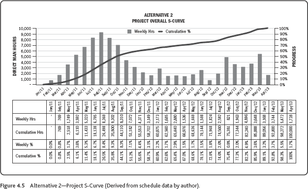
4.3.2 Alternative 2 Project S-Curve
Using the output from the developed Primavera file for weekly and cumulative man hours, the S-curve shown in Figure 4.5 has been developed for Alternative 2.
4.3.3 Cost/Earned Value Management Of Alternative 2
Original Budget = 363,014,661
At the 25% stage of the project:
Planned Value (PV) = 90,753,665
Earned Value (EV) = 36,301,466 (indicating 10% project completion)
Actual Cost (AC) = 46,301,466
Schedule Performance Index (SPI) = EV/PV = 0.4 (behind schedule)
Cost Performance Index (CPI) = EV/AC = 0.78 (over budget)
Forecasted Estimate at Completion at This Stage = BAC/CPI = 465,403,411
At the 50% stage of the project:
Planned Value (PV) = 181,507,330
Earned Value (EV) = 108,904,398 (indicating 30% project completion)
Actual Cost (AC) = 145,205,865
Schedule Performance Index (SPI) = EV/PV = 0.6 (behind schedule)
Cost Performance Index (CPI) = EV/AC = 0.75 (over budget)
Forecasted Estimate at Completion at this Stage = BAC/CPI = 484,019,548
At the 75% stage of the project:
Planned Value (PV) = 272,260,995
Earned Value (EV) = 235,959,529 (indicating 65% project completion)
Actual Cost (AC) = 272,260,995
Schedule Performance Index (SPI) = EV/PV = 0.86 (behind schedule)
Cost Performance Index (CPI) = EV/AC= 0.86 (over budget)
Forecasted Estimate at Completion at this stage = BAC/CPI = 422,110,070
At the 100% stage of the project:
Planned Value (PV) = Budget at Completion (BAC) = 363,014,661
Earned Value (EV) = 363,014,661
Actual Cost (AC) = 420,110,070
Schedule Performance Index (SPI) = EV/PV = 1.00 (It is interesting to see that the SPI equals 1 for this alternative even when the project has delayed because we are calculating SPI at the 100% stage, that is, when the project has already been completed.
Cost Performance Index (CPI) = EV/AC = 0.86.
4.3.4 Observations
Therefore, from the simulation of Alternative 2, we see the following:
- The project is completed four months late and after the deadline on April 28.
- The project comes in over budget as a result of improper planning, mismanagement of resources, idle worker hours, and delays in the receipt of materials.
- It is pertinent to mention here that according to Section 3.1 of this study, the contract is a fixed price with incentive type and a penalty/liquidated damages of 0.1% of contract price per day late completed was stipulated on this contract up to a maximum of 10% of the contract price. Thus, the value of the penalty that the project suffered was:
Liquidated damages for 120 days = 0.1% of 363,014,661 × 120 = 43,561,759
However, it must be noted here that there is a 10% slab on bonus/penalties enforced by the contract, which is applicable in this case. Therefore, 10% of 363,014,661 = 36,301,466.
Thus, the net actual value of the project is as follows:
Revised Actual Cost = 420,110,070 + 36,301,466 = 456,411,536
That is, there is a loss of 93,396,875.
Revised CPI at completion = 0.79 (i.e., the project is completed over budget)
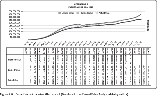
The Earned Value Analysis of the Alternative 2 Project simulation is shown in Figure 4.6.
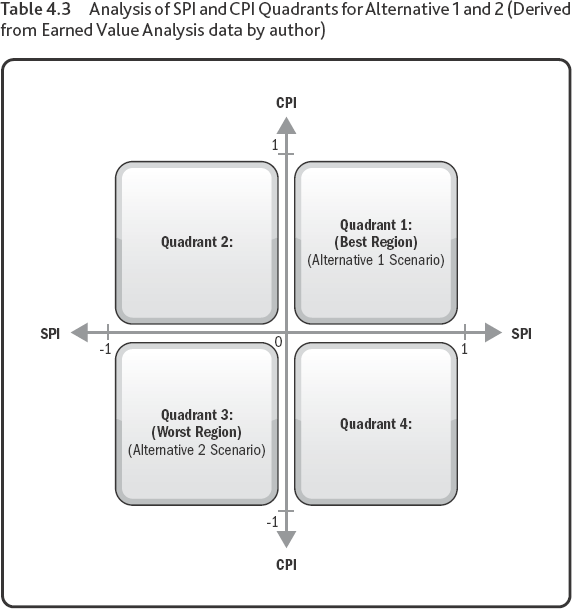
Table 4.3 shows the CPI and SPI Quadrant Analysis of both alternatives toward the end of the project.