6 The Product/Service Plan

You have a choice of four different types of mousetraps to catch your customers. They are:

1. A better mousetrap

2. A disappearing-mouse mousetrap

3. A 36-inch mousetrap

4. A cheaper mousetrap

A better mousetrap is of higher quality than the competition. Examples are Haagen Dazs ice cream, Godiva chocolates, and Cross pens. A disappearing-mouse mousetrap is where you don’t have to see the dead mouse. You can now buy mousetraps where the mouse goes into a box, like a little hotel, and can’t get back out in the morning. Then you throw out the hotel. This type of mousetrap is not any more effective than the old kind, but is preferred because you don’t see the dead mouse. The definition of a disappearing-mouse mousetrap is a product or service that is actually not superior to competition, but is believed to be so, due to effective marketing. Examples are Marriott Hotels, Budweiser, and British Airways.

You beer drinkers who don’t like the taste of Bud and want to argue with me about classifying Budweiser as a disappearing-mouse mousetrap, you have to remember they have the largest market share of any beer.

A 36-inch mousetrap is a niche player. Examples are Hasselblad cameras, Montessori schools, and Panera Bread. A cheaper mouse trap is self-explanatory. Examples are Wal-Mart, Days Inn, and Target.

To become one of these four types of mousetraps takes money. For example, if you want to be a better mousetrap, you have to improve your business operation, either your manufacturing process, customer service, or some other aspect. At Marriott, customer service is an attitude, not a department. “Marriott is the most reliable of brands,” says Bjorn Hanson, an industry analysis who now teaches at New York University’s Tisch Center for Hospitality, Tourism, and Sports Management. “There is a saying in the industry that Marriott puts heads in beds.”¹

To become a disappearing-mouse mousetrap, you have to become more effective in marketing. Who doesn’t love those Budweiser Clydesdales? To be a successful niche player, you have to have high quality and a large market share. Digital cameras have replaced film, but the Hasselblad is the camera that they took to the moon. Mention Panera Bread and fans are as likely to praise the free Wi-Fi as they are to gush about the Asiago cheese bagels. And that, execs at the $2.6 billion restaurant chain say, is the point. While its competitors scale back on upscale ingredients, trim portion sizes, and create value menus, Panera is selling fresh food and warm bread at full price and encouraging customers to linger. That recipe is succeeding.²

Responding to competition, Starbucks is now starting to offer free Wi-Fi in their stores.

To be a cheaper mousetrap, you have to increase your productivity so you will be the best in operational efficiency. Wal-Mart has more screens at their home base than the three television networks combined. They show every step of their distribution process around the world.

Because more expenditures are needed to execute any of these strategies, a good system to use is the experience curve to determine whether the costs are justifiable. The experience curve concept was initially labeled the learning curve. During World War II, an Air Force general recognized that as we kept assembling more and more B-17 bombers, the workforce was able to assemble each one in less time. As labor spent more time on the job, they became more adept at what they were doing, adapted better processes, became more specialized, and so on. The result was increased productivity. This concept is considered just common sense today, but back then it was revolutionary.

In subsequent years, management realized that savings due to increased productivity were possible from many areas besides labor. There were economies of scale. If a 10-million-ton oil refinery cost $10 million to build and took 5,000 employees to operate, a 20-million-ton refinery does not cost $20 million to build and take 10,000 employees to operate. Rather, approximately $15 million and 7,500 employees. As companies bought larger amounts from their suppliers, they could demand lower prices and better terms. Marketing costs could also be lowered. It doesn’t cost ten times as much to advertise ten stores in a city as it does for one.

The sum of all these savings is referred to as “the experience curve” and the concept is that in industries where these savings are applicable and you take advantage of them, your costs will decrease approximately the same percent each time you double your volume. If your costs in real dollars after you double your volume are 85 percent of previous figures, then you are on an 85 percent experience curve. Notice that it’s based on doubling of volume, not on time. Therefore, you can use the experience curve to check the feasibility of adapting one of the above strategies.

Calculating the Experience Curve

To begin, you should determine what experience curve rate you are currently on based on past costs versus today’s costs. Let’s look at the first case history, in CEXCURVE.xls, concerning a hypothetical company called Strategic Business Unit (SBU).

The experience curve for this company, SBU, is 89.01 percent. Their operation has three components. There is one component A per unit, two components B, and one component C, which is supplied by an outside supplier. The experience curve for component A is 84.34 percent, 87.36 percent for component B, 81.90 percent for component C, and 89.01 percent in total. (Yes, the total experience curve is calculated independently, from the total costs themselves; it is not an average—weighted or otherwise—of the first three curves.)

Let’s examine in detail how the computer model performs. Component A costs $50 in 2002 and $30 in 2009. The experience curve concept is that costs are decreased at the same percentage rate each time cumulative volume is doubled. First-year volume (2002) for SBU X (our new product’s name) was 1,000 units. There is one component A per unit so first-year volume on component A was also 1,000. First-year volume is the base on which all subsequent doubling is calculated. In 2003, volume on component A was 2,100 and the computer model recognizes that the first doubling in volume occurs (from 1,000 the first year to 2,100 cumulative by the end of the second year). The second doubling will occur when cumulative volume hits 4,000 and this happens in 2005. The third doubling will be 8,000 and this level is reached in 2008. The question to the computer model is: at what experience curve rate are costs being reduced if a component’s cost is reduced from $50 to $30 during a period of three doublings? The answer is 84.34 percent, as shown in the exhibit directly under the column “# units” for component A. If you want to verify the computer model’s math, multiply $50 by 84.34 percent and you will get $42.17. This should be the cost of component A after the first doubling, which occurs in 2003. Verify this cost on the exhibit. The cost after the second doubling (2005) should be $42.17 times 84.34 percent or $35.57, and the third doubling (2008), $35.57 times 84.34 percent or $30. Isn’t math gratifying?

The computer model does the same calculations for component B, component C, and the sum of components A, B, and C or total cost of SBU X. For component B, two units are used for each unit of SBU X, so the first doubling occurs at 4,000 (first-year volume of 2,000 times 2) rather than the 2,000 level for component A (first-year volume of 1,000 times 2). However, even though each doubling is achieved at higher levels (first: 4,000; second: 8,000; third: 16,000; and so on) than for component A, because two units are used per unit of SBU X, component B reaches each doubling at the same time as component A.

This is not true for component C. First-year volume is 1,000 because one component is used per SBU X unit. However, the company that supplies this component to the company had produced 4,000 for use with other products before 2002. Therefore, the first-year volume is listed at 5,000 and the first doubling does not occur until 10,000 units. This level is not reached until 2006 (10,105 cumulative volume). Although the experience curve rate or cost reduction for each doubling is greater for component C (81.90 percent) than for A (84.34 percent) or B (87.36 percent), only one doubling is obtained during the period 2002 to 2009, and the cost is only reduced from $105 to $86 ($105 times 81.90 percent). The combined experience curve rate for SBU X is 89.01 percent and total cost of goods is reduced from $329 to $232 during these eight years (2002 to 2009).

This experience curve rate for the components can now be used for future costs projections. SBU can estimate that when they reach the fourth doubling (16,000), the cost for component A should be approximately $25.30 ($30 times 84.34 percent); fifth doubling, $21.34 ($25.30 times 84.34 percent); and so on.

When you use this part of the model EXCURVE.xls for your own SBUs, you may find that you have experienced no cost reductions, even after adjusting the numbers for inflation. This would probably mean that either the experience curve concept does not exist in your particular market or it does but you are not taking advantage of it. In some industries it’s difficult, if not impossible, to experience savings from economies of scale, although the number of industries appears to be small. An example would be most restaurants because they tend to be labor-intensive and have high staff turnover. On the other hand, the economies could be there in your particular industry, but you have failed to realize it. Maybe you are not demanding lower costs from your suppliers due to your increased volume nor are you aggressively promoting your firm to top prospective new employees. Maybe you have not organized your company to profit from economies of scale in manufacturing, operations, advertising, distribution, sales promotion, etc.

From your books or accountant, insert your own data in the Excel file EXCURVE.xls. Only insert your data where you see the blue zeros or lines. All black zeros are formulas.

After you insert your numbers, the experience curve rate will be calculated automatically. If you have more components than shown above, just copy and paste. If you are a service company, you can change the word “component” to “service offered,” “customer service,” etc.

For comparison purposes, you can project yourself into the future doing what you are doing now and then compare these numbers with those of the various strategies you want to consider. The case history of our hypothetical SBU, we postulate that it is growing at the rate of 10 percent per year (see Figures 6–1 and 6-2). The projection of how this will play out in succeeding years is shown in Figure 6–3.

Now we will take a look at their complete operation, as seen in Figure 6–4. It includes the total costs, pricing, market share, and profits for our SBU.

Calculating Discounted Cash Flow

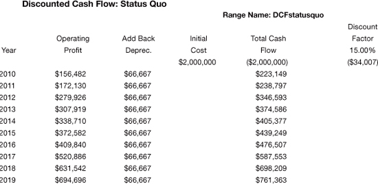
Our third and final file for the status quo shows the discounted cash flow of this plan (see Figure 6–5). Discounted cash flow is probably the single most important number that will come out of this chapter.

This is not a bad plan. If the SBU just continues doing what they have in the past, their discounted cash flow is 15 percent. Discounted cash flow is your return on your investment over time. When you complete these same three files for your company and you obtain a similar rate of return, you may not want to make any changes. Of course, if you obtain a lower rate of return, most likely you should consider changes.

I believe discounted cash flow is the most meaningful measurement of success. Profit is something made up by accountants. Try buying something at the grocery store with that figure. Besides, it doesn’t take into account committed resources or time. Return on investment (ROI) adds resources to the equation, but does not consider time, and once again, it’s an accounting term. However, cash flow is that green stuff in your pocket and that’s what really counts. Adding time to cash flow gives you discounted cash flow or the rate of return on your resources invested over a given period of time. Calculating discounted cash flow on various plans also allows you to compare apples and oranges. If plan A is to raise apples with an initial investment of $100,000 and estimated DCF of 20 percent over five years, everything else being equal, it’s better than plan B, which is to raise oranges with an initial investment of $75,000 and estimated DCF of 10 percent over the same period of time.

Figure 6–1 Past cost of goods experience—SBU (CEXCURVE; range name: SBUpastcosts).

Figure 6–2 Your past cost of goods experience—SBU (EXCURVE, range name: SBUpastcosts).

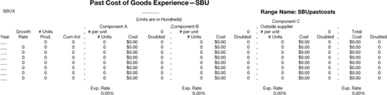
Figure 6–3 Estimated cost of goods experience—status quo (CEXCURVE; range name: Growthstatusquo).

Figure 6–4 Status quo strategy (CEXCURVE; range name: SBUstatusquo).

Figure 6–5 Discounted cash flow: status quo (CEXCURVE; range name: DCFstatusquo).

Figures 6-6, 6-7, and 6-8 are facsimiles of the three files we have just discussed into which you will put your data to compute your status quo.

Remember, only insert data where you see blue zeros. To calculate your discounted cash flow factor, keep putting percent numbers under the wording “Discount Factor” until the number below is the smallest you can obtain. For example, on Figure 6–5 the discount factor (last column on the right) is 15 percent and the number below that is 34,007. (Note that this number does not represent dollars; it is just a number, and your goal, for various arcane mathematical reasons, is to minimize it.) If you insert 16 percent instead of 15 percent, the number below becomes –123,940. If you insert 14 percent, the number becomes 62,352. Therefore, 15 percent is correct.

Figure 6–6 Your estimated future cost of goods experience—status quo (EXCURVE; range name: Growthstatusquo).

Figure 6–7 Your status quo strategy (EXCURVE; range name: SBUstatusquo).

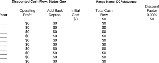
Figure 6–8 Your discounted cash flow: status quo (EXCURVE; range name: DCFstatusquo).

The computer model has files for six different experience curve strategies and a composite that adds all the strategies you complete into one. They are pricing (growthpricing), sales (growthsales), promotion (growthpromotion), vertical integration (growthvalueadded), manufacturing/engineering (growthmfgeng), customer service/distribution (growthcsdist) and the composite (growthcomposite).

Following are the case history files for the pricing strategy.

Calculating a Pricing Strategy

Let’s assume one of your markets is sensitive to price; you are in a position to absorb a loss for a few years; and you don’t believe your competitors can or will match a price cut on your part. Let’s further assume that if you lower your price from $400 to $270 for two years and then to $235 for another three years, you could increase your annual growth rate from 10 percent to 30 percent. Probably by the end of this five-year plan your competitors would be forced out of the market, at which time you would increase your price to $410. (Probably excessive numbers, but the theory is the same.)

Based on these assumptions, you can use the Excel file to determine what would be the DCF for this price-cutting strategy. As you can see in Figure 6–9, we inserted the above-mentioned growth rate (30 percent) in the growth rate column. The computer then calculates, based on the experience curve rate (determined back in Figure 6–1, what your costs of goods would be in subsequent years. As Figure 6–9 shows, costs for our hypothetical SBU would be driven from $232 in 2009 to $142.59 in 2019.

Because we are considering a price-cutting strategy here, we will keep all other costs the same as in the past on a per unit basis. For example, as shown in Figure 6–10, SBU has been spending $50 per unit on sales activity and plans to keep it at this level. Next we have inserted a sales price and estimated industry growth rate. This enables the computer to calculate SBUs operating profit and market share. As we see in Figure 6–10, market share increases from 25 percent to 58 percent.

We can now check on the financial soundness of this strategy. We go to Discounted Cash Flow: Price (range name: DCF-price) (see Figure 6–11), and insert the investment needed to execute this plan for the status quo plan, which is $2,000,000. In a pricing strategy such as this one, total investment and operating profit, rather than just incremental investment and operating profit resulting from the new strategy, is used in calculating DCF. This is because a price cut affects the previous base of business as well as any new business. For the other types of strategies only incremental investment and operating profit will be used on calculating DCF. Then we inserted non-cash expenditures, in this case depreciation, and the computer calculates the DCF for the plan. In the case history, it is 16 percent.

Figure 6–9 Estimated cost of goods experience—SBU pricing (CEXCURVE; range name: Growthpricing).

Figure 6–10 Pricing strategy (CEXCURVE; range name: SBUpricing).

Figure 6–11 Discounted cash flow: Price (CEXCURVE; range name: DCFprice).

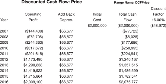
The discounted cash flow rate is only 16 percent for this pricing strategy, just one point above the status quo of 15 percent. Unless you made a mistake in your calculations or want to make some changes in the strategy, this activity does not make financial sense. That is the value of these files. You keep trying different strategies until you obtain a good financial return.

You may have noticed that no tax was taken out of operating income. To calculate true DCF, you should go to EXCURVE.xls (range name DCFprice) and fill in your data as we have done in Figure 6–11. Because there is such a wide variation on how tax is calculated for various companies, this has not been included in the model.

What If…?

Following are five additional strategies that you can experiment with by asking yourself what if I did this or that. You are looking for the one that gives you your best discounted case flow. The strategies are value added, promotion, sales, customer service/distribution and manufacturing/engineering. You should look at the case histories first on Cexcurve.xls and then go to Excurve.xls and fill in your data.

Value Added

The primary reason for vertical integration is to increase value added because the higher the value added, everything else being equal, the higher the ROI.

There are two ways to vertically integrate: backward (“upstream”) and forward (“downstream”). If you are a paper manufacturer, an example of upstream integration is the growing of trees and of downstream, the purchase or development of retail stores that sell your paper. The major factor to consider in integration is margins (operating profit before taxes expressed as a percent of total sales or revenues). You normally want to go in the direction of the highest margins and they usually increase as you move closer to the end user of your product or service. If you integrate upstream, the product or service is normally more of a commodity and therefore price is a major factor and margins are small. Conversely, if you market your products to the retail trade, such as Reynolds Metals (Reynolds Wrap and a host of other consumer products), you can enjoy margins as high as 30 to 40 percent. However, you have to understand the business. DuPont decided to sell the core of their business—nylon and textiles—and became a “science company.” I cannot find an explanation for the switch, but it has not gone very well for them. They moved from a market they knew and were strong in to a market they don’t know that well and are not strong in. They were profitable the last two quarters, but their stock price is lower than it was seven years ago.

Recently, companies have become more prone to go vertical. Oracle Corporation bought Sun Microsystems to transform the company into a maker of software, computers, and computer components. Pepsi is buying distributors because they want more control over distribution. Boeing purchased Vought Aircraft Industries to add control over manufacturing and Apple bought P.A. Semi for their customized microprocessors.

Value added is the percent of the selling price that you add to cover your own activity. If you buy raw materials for $200 and fabricate them into a machine that you sell for $1,000, your value added is 80 percent. Therefore, the more you integrate, the higher your value added.

Now, returning to our case study of SBU X, it is estimated that by executing a vertical integration strategy and a slight reduction in price based on resulting cost savings, annual sales growth can be increased from the current 10 percent to 13 percent for five years and then back to 10 percent for the next five years. This is shown in the CEXCURVE.xls file “Estimated Future Cost of Goods Experience—Value Added” (range name: Growthvalueadded). This increased sales volume would lower costs of goods from $232 to $167.56 by 2019.

In the CEXCURVE, “Value Added Strategy” (range name: SBUvalueadded), the anticipated cost savings of $10 per unit for the years 2010 to 2013 and $15 for 2014 to 2019 are shown. Price has been decreased from $400 to $390 beginning in 2010 and to $385 in 2014. The financials for this strategy are shown in the Excel file “Discounted Cash Flow: Value Added” (range name: DCFvalueadded). The incremental DCF rate is 27 percent.

Promotion Strategy

Nobody does it better than Procter & Gamble. Although they usually launch with a superior product, it is the power of their advertising and sales promotion that makes them either one or two in market share in most of their markets. However, once again, you have to know what you are doing. Texas Instruments, a technology-driven company, tried three times to crack consumer markets (hand-held calculators, watches, and personal computers for the home) and failed miserably each time. After announcing they were getting out of consumer marketing, their stock increased $50 the next day.

Returning to our case study of SBU X, it is estimated that by executing a heavy promotion strategy, annual sales growth can be increased from the current 10 percent to 14 percent for five years and then back to 10 percent for the next five years. This is shown in the CEXCURVE file “Estimated Future Cost of Goods Experience—Promotion” (range name: Growthpromotion). This increased sales volume would lower costs of goods from $232 to $167.56 by 2019.

In the CEXCURVE file “Promotion Strategy” (range name: SBUpromotion), promotion expenditures per unit have been increased from the current $20 to $50 for the period 2010 to 2014 and dropped back to $20 for the period 2015 to 2019. The resulting share increase is from the current 25 percent to 30 percent in 2019.

This is one of the strategies behind the introduction of Fresca, the Coca-Cola Company soft drink. Fresca was the first successful non-sugar soft drink. Sugar accounts for over 50 percent of ingredient costs in a soft drink and consequently the Coca-Cola Company could afford a much higher per unit advertising expenditure on Fresca. The drink was very successful until the company had to change the formula due to the ban on cyclamates.

The financials for this strategy are shown in the Excel file “Discounted Cash Flow: Promotion” (range name: DCFpromotion). The incremental DCF rate is only 15 percent.

Sales Strategy

Maybe emphasis on sales is the direction to go, like IBM (consulting). Sales activity can be inserted into the Excel file. The range names are in the upper right-hand corner of the charts (growthsales, SBUsales, and DCFsales). In the case history, a growth rate increase from the current 10 percent to 16 percent is projected for five years. Sales expense has been increased from $50 to $100 per unit. Projected share increase is from 25 percent to 33 percent and the resulting incremental DCF is 12 percent.

Customer Service/Distribution Strategy

Disney, British Airways, and Marriott know the power of customer service. Fed Ex and Wal-Mart know the power of unique distribution.

This section is covered in the Excel file (range names: growthcsdist, SBUcsdist, and DCFcsdist) as well. In the case history, increased growth rate is projected from the current 10 percent to 13 percent for five years. Customer service/distribution costs are increased from $5 to $18 per unit. Share increases from 25 percent to 29 percent, and the DCF for this execution is estimated at 24 percent.

Manufacturing/Engineering Strategy

Here comes the better mousetrap; the best strategy of all if you can pull it off. Use the following ranges for your attempt to find a better mousetrap (range names: growthmfgeng, SBUmfgeng, and DCFmfgeng). For SBU X, it is estimated that they will achieve the best DCF with an investment of $350,000 (too bad it isn’t quite that simple). Growth rate increases to 14 percent and share to 29 percent. They are even able to reduce their manufacturing costs $12 per unit. The incremental DCF is 33 percent.

If you are considering developing a new product or service, these files will help you determine your project goals and with research, you can maintain close contact with your customers as the following company, a medical-device manufacturer, did. This company created a matrix to identify and weigh the importance of various features to different customer segments. It then tested trade-offs between product and things like price with various medical specialists who used the product in simulated clinical settings. That allowed the team to fine-tune the product well before launch for medical testing.³

Composite of Above Strategies

On the composite range names, all the previous strategies except for the pricing strategy are added together and we get the final results (range names: growthcomposite, SBUcomposite, and DCFcomposite). There’s no need to add anything to growthcomposite because all its data is picked up from other ranges. On SBUcomposite, everything is picked up except the new sales price, the industry growth, and the beginning share. On DCFcomposite, one only has to insert the right DCF rate.

In the case history, the total growth rate is 30 percent for five years and then levels off at 10 percent for the remaining five. Cost of goods goes down from $232 in 2009 to $142.50 in 2019. Total costs, even with all this new activity, goes from $424 in 2002 to just $213 in 2019. Market share increases to 58 percent (you own the market) and the incremental DCF is 30 percent.

The discounted cash flow of each strategy can be charted with Excel’s charting function as seen in Figure 6–12. This is one of seven charts on the various strategies available on the CEXCURVE file.

For at least some of you, using the experience curve can give you great savings. For example, the computer chip industry is on a very high experience curve rate cost reduction, probably in the neighborhood of 50 percent. That means that every time you double your volume, your costs are 50 percent lower. Today you can hold in the palm of your hand a computer chip that has more power than a computer manufactured forty years ago that was so large it would have filled six to ten bedrooms. If the American automobile industry had pushed the experience curve similar to the computer industry, a Cadillac today would cost $50 and be able to drive around the world on one tank of gas.

Figure 6–12 Discounted cash flow by strategy (CEXCURVE; chart name: DCFfunctions).

The discounted cash flow rate for these various strategies has nothing to do with the feasibility or possible effectiveness that they would have in your market. They are just case histories showing how to calculate the results.

Following is a worksheet for your product/service plan. You can photocopy this one, or print out a copy from the Worksheets folder you downloaded. (Okay, one last time: www.amacombook.org/go/MarketingPlan4.) You can change my categories if appropriate, and you should probably not put in volume and share until after you go through the upcoming sales plan chapters (Chapters 12 and 13). By “type of mousetrap,” I mean which of the four approaches discussed above is going to be your thrust.

Worksheet 6–1 Product/service plan: Objectives and strategies

Notes

1. Marc Gunther, “Marriott Gets a Wake-Up Call,” Fortune, July 6, 2009; http://money.cnn.com/2009/06/22/news/companies/marriott_hotels_makeover.fortune/?postversion=2009062508.

2. Kate Rockwood, “Rising Dough, Why Panera Bread Is on a Roll,” Fast Company, October 2009; http://www.fastcompany.com/magazine/139/rising-dough.html.

3. Mike Gordon, Chris Musso, Eric Rebentisch, and Nisheeth Gupta, “The Path to Developing Successful New Products,” Wall Street Journal, November 30, 2009; http://online.wsj.com/article/NA_WSJ_PUB:SB10001424052970203440104574400593760720388.html#articleTabs%3Darticle.