12

Simulation and Optimization Competitions

Reinforcement learning (RL) is an interesting case among the different branches of machine learning. On the one hand, it is quite demanding from a technical standpoint: various intuitions from supervised learning do not hold, and the associated mathematical apparatus is quite a bit more advanced; on the other hand, it is the easiest one to explain to an outsider or layperson. A simple analogy is teaching your pet (I am very intentionally trying to steer clear of the dogs versus cats debate) to perform tricks: you provide a treat for a trick well done, and refuse it otherwise.

Reinforcement learning was a latecomer to the competition party on Kaggle, but the situation has changed in the last few years with the introduction of simulation competitions. In this chapter, we will describe this new and exciting part of the Kaggle universe. So far – at the time of writing – there have been four Featured competitions and two Playground ones; this list, while admittedly not extensive, allows us to give a broad overview.

In this chapter, we will demonstrate solutions to the problems presented in several simulation competitions:

• We begin with Connect X.
• We follow with Rock, Paper, Scissors, where a dual approach to building a competitive agent is shown.
• Next, we demonstrate a solution based on multi-armed bandits to the Santa competition.
• We conclude with an overview of the remaining competitions, which are slightly outside the scope of this chapter.

If reinforcement learning is a completely new concept for you, it is probably a good idea to get some basic understanding first. A very good way to start on the RL adventure is the Kaggle Learning course dedicated to this very topic in the context of Game AI (https://www.kaggle.com/learn/intro-to-game-ai-and-reinforcement-learning). The course introduces basic concepts such as agents and policies, also providing a (crash) introduction to deep reinforcement learning. All the examples in the course use the data from the Playground competition Connect X, in which the objective is to train an agent capable of playing a game of connecting checkers in a line (https://www.kaggle.com/c/connectx/overview).

On a more general level, it is worth pointing out that an important aspect of simulation and optimization competitions is the environment: due to the very nature of the problem, your solution needs to exhibit more dynamic characteristics than just submitting a set of numbers (as would be the case for “regular” supervised learning contests). A very informative and detailed description of the environment used in the simulation competitions can be found at https://github.com/Kaggle/kaggle-environments/blob/master/README.md.

Connect X

In this section, we demonstrate how to approach the simple problem of playing checkers using heuristics. While not a deep learning solution, it is our view that this bare-bones presentation of the concepts is much more useful for people without significant prior exposure to RL.

If you are new to the concept of using AI for board games, the presentation by Tom van de Wiele (https://www.kaggle.com/tvdwiele) is a resource worth exploring: https://tinyurl.com/36rdv5sa.

The objective of Connect X is to get a number (X) of your checkers in a row – horizontally, vertically, or diagonally – on the game board before your opponent. Players take turns dropping their checkers into one of the columns at the top of the board. This means each move may have the purpose of trying to win for you or trying to stop your opponent from winning.

Figure 12.1: Connect X board

Connect X was the first competition that introduced agents: instead of a static submission (or a Notebook that was evaluated against an unseen dataset), participants had to submit agents capable of playing the game against others. The evaluation proceeded in steps:

1. Upon uploading, a submission plays against itself to ensure it works properly.
2. If this validation episode is successful, a skill rating is assigned, and the submission joins the ranks of all competitors.
3. Each day, several episodes are played for each submission, and subsequently rankings are adjusted.

With that setup in mind, let us proceed toward demonstrating how to build a submission for the Connect X competition. The code we present is for X=4, but can be easily adapted for other values or variable X.

First, we install the Kaggle environments package:

!pip install kaggle-environments --upgrade

We define an environment in which our agent will be evaluated:

from kaggle_environments import evaluate, make
env = make("connectx", debug=True)
env.render()

While a frequent impulse you might have is to try sophisticated methods, it is useful to start simple – as we will do here, by using simple heuristics. These are combined into a single function in the accompanying code, but for the sake of presentation, we describe them one at a time here.

The first rule is checking whether either of the players has a chance to connect four checkers vertically and, if so, returning the position at which it is possible. We can achieve this by using a simple variable as our input argument, which can take on two possible values indicating which player opportunities are being analyzed:

def my_agent(observation, configuration):
    from random import choice
    # me:me_or_enemy=1, enemy:me_or_enemy=2
    def check_vertical_chance(me_or_enemy):
        for i in range(0, 7):
            if observation.board[i+7*5] == me_or_enemy 
            and observation.board[i+7*4] == me_or_enemy 
            and observation.board[i+7*3] == me_or_enemy 
            and observation.board[i+7*2] == 0:
                return i
            elif observation.board[i+7*4] == me_or_enemy 
            and observation.board[i+7*3] == me_or_enemy 
            and observation.board[i+7*2] == me_or_enemy 
            and observation.board[i+7*1] == 0:
                return i
            elif observation.board[i+7*3] == me_or_enemy 
            and observation.board[i+7*2] == me_or_enemy 
            and observation.board[i+7*1] == me_or_enemy 
            and observation.board[i+7*0] == 0:
                return i
        # no chance
        return -99

We can define an analogous method for horizontal chances:

    def check_horizontal_chance(me_or_enemy):
        chance_cell_num = -99
        for i in [0,7,14,21,28,35]:
            for j in range(0, 4):
                val_1 = i+j+0
                val_2 = i+j+1
                val_3 = i+j+2
                val_4 = i+j+3
                if sum([observation.board[val_1] == me_or_enemy, 
                        observation.board[val_2] == me_or_enemy, 
                        observation.board[val_3] == me_or_enemy, 
                        observation.board[val_4] == me_or_enemy]) == 3:
                    for k in [val_1,val_2,val_3,val_4]:
                        if observation.board[k] == 0:
                            chance_cell_num = k
                            # bottom line
                            for l in range(35, 42):
                                if chance_cell_num == l:
                                    return l - 35
                            # others
                            if observation.board[chance_cell_num+7] != 0:
                                return chance_cell_num % 7
        # no chance
        return -99

We repeat the same approach for the diagonal combinations:

# me:me_or_enemy=1, enemy:me_or_enemy=2
def check_slanting_chance(me_or_enemy, lag, cell_list):
        chance_cell_num = -99
        for i in cell_list:
            val_1 = i+lag*0
            val_2 = i+lag*1
            val_3 = i+lag*2
            val_4 = i+lag*3
            if sum([observation.board[val_1] == me_or_enemy, 
                    observation.board[val_2] == me_or_enemy, 
                    observation.board[val_3] == me_or_enemy, 
                    observation.board[val_4] == me_or_enemy]) == 3:
                for j in [val_1,val_2,val_3,val_4]:
                    if observation.board[j] == 0:
                        chance_cell_num = j
                        # bottom line
                        for k in range(35, 42):
                            if chance_cell_num == k:
                                return k - 35
                        # others
                        if chance_cell_num != -99 
                        and observation.board[chance_cell_num+7] != 0:
                            return chance_cell_num % 7
        # no chance
        return -99

We can combine the logic into a single function checking the opportunities (playing the game against an opponent):

    def check_my_chances():
        # check my vertical chance
        result = check_vertical_chance(my_num)
        if result != -99:
            return result
        # check my horizontal chance
        result = check_horizontal_chance(my_num)
        if result != -99:
            return result
        # check my slanting chance 1 (up-right to down-left)
        result = check_slanting_chance(my_num, 6, [3,4,5,6,10,11,12,13,17,18,19,20])
        if result != -99:
            return result
        # check my slanting chance 2 (up-left to down-right)
        result = check_slanting_chance(my_num, 8, [0,1,2,3,7,8,9,10,14,15,16,17])
        if result != -99:
            return result
        # no chance
        return -99

Those blocks constitute the basics of the logic. While a bit cumbersome to formulate, they are a useful exercise in converting an intuition into heuristics that can be used in an agent competing in a game.

The performance of our newly defined agent can be evaluated against a pre-defined agent, for example, a random one:

env.reset()
env.run([my_agent, "random"])
env.render(mode="ipython", width=500, height=450)

The code above shows you how to set up a solution from scratch for a relatively simple problem (there is a reason why Connect X is a Playground and not a Featured competition). Interestingly, this simple problem can be handled with (almost) state-of-the-art methods like AlphaZero: https://www.kaggle.com/connect4alphazero/alphazero-baseline-connectx.

With the introductory example behind us, you should be ready to dive into the more elaborate (or in any case, not toy example-based) contests.

Rock-paper-scissors

It is no coincidence that several problems in simulation competitions refer to playing games: at varying levels of complexity, games offer an environment with clearly defined rules, naturally lending itself to the agent-action-reward framework. Aside from Tic-Tac-Toe, connecting checkers is one of the simplest examples of a competitive game. Moving up the difficulty ladder (of games), let’s have a look at rock-paper-scissors and how a Kaggle contest centered around this game could be approached.

The idea of the Rock, Paper, Scissors competition (https://www.kaggle.com/c/rock-paper-scissors/code) was an extension of the basic rock-paper-scissors game (known as roshambo in some parts of the world): instead of the usual “best of 3” score, we use “best of 1,000.”

We will describe two possible approaches to the problem: one rooted in the game-theoretic approach, and the other more focused on the algorithmic side.

We begin with the Nash equilibrium. Wikipedia gives the definition of this as the solution to a non-cooperative game involving two or more players, where each player is assumed to know the equilibrium strategies of the others, and no player can obtain an advantage by changing only their own strategy.

Denoting our players as red and blue, each cell in the matrix of outcomes shows the result of a given combination of moves:

Figure 12.2: Payoff matrix for rock-paper-scissors

As an example, if both play Rock (the top-left cell), both gain 0 points; if blue plays Rock and red plays Paper (the cell in the second column of the first row), red wins – so red gains +1 point and blue has -1 point as a result.

If we played each action with an equal probability of 1/3, then the opponent must do the same; otherwise, if they play Rock all the time, they will tie against Rock, lose against Paper, and win against Scissors – each with a probability of 1/3 (or one-third of the time). The expected reward, in this case, is 0, in which case we can change our strategy to Paper and win all the time. The same reasoning can be conducted for the strategy of Paper versus Scissors and Scissors versus Rock, for which we will not show you the matrix of outcomes due to redundancy.

The remaining option in order to be in equilibrium is that both players need to play a random strategy – which is the Nash equilibrium. We can build a simple agent around this idea:

%%writefile submission.py
import random
def nash_equilibrium_agent(observation, configuration):
    return random.randint(0, 2)

How does our Nash agent perform against others? We can find out by evaluating the performance:

!pip install -q -U kaggle_environments
from kaggle_environments import make

We start by creating the rock-paper-scissors environment and setting the limit to 1,000 episodes per simulation:

env = make(
    "rps", 
    configuration={"episodeSteps": 1000}
)

We will make use of a Notebook created in this competition that implemented numerous agents based on deterministic heuristics (https://www.kaggle.com/ilialar/multi-armed-bandit-vs-deterministic-agents) and import the code for the agents we compete against from there:

%%writefile submission_copy_opponent.py
def copy_opponent_agent(observation, configuration):
    if observation.step > 0:
        return observation.lastOpponentAction
    else:
        return 0
# nash_equilibrium_agent vs copy_opponent_agent
env.run(
    ["submission.py", "submission_copy_opponent.py"]
)
env.render(mode="ipython", width=500, height=400)

When we execute the preceding block and run the environment, we can watch an animated board for the 1,000 epochs. A snapshot looks like this:

Figure 12.3: A snapshot from a rendered environment evaluating agent performance

In supervised learning – both classification and regression – it is frequently useful to start approaching any problem with a simple benchmark, usually a linear model. Even though not state of the art, it can provide a useful expectation and a measure of performance. In reinforcement learning, a similar idea holds; an approach worth trying in this capacity is the multi-armed bandit, the simplest algorithm we can honestly call RL. In the next section, we demonstrate how this approach can be used in a simulation competition.

Santa competition 2020

Over the last few years, a sort of tradition has emerged on Kaggle: in early December, there is a Santa-themed competition. The actual algorithmic side varies from year to year, but for our purposes, the 2020 competition is an interesting case: https://www.kaggle.com/c/santa-2020.

The setup was a classical multi-armed bandit (MAB) trying to maximize reward by taking repeated action on a vending machine, but with two extras:

• Reward decay: At each step, the probability of obtaining a reward from a machine decreases by 3 percent.
• Competition: You are constrained not only by time (a limited number of attempts) but also by another player attempting to achieve the same objective. We mention this constraint mostly for the sake of completeness, as it is not crucial to incorporate explicitly in our demonstrated solution.

The solution we demonstrate is adapted from https://www.kaggle.com/ilialar/simple-multi-armed-bandit, code from Ilia Larchenko (https://www.kaggle.com/ilialar). Our approach is based on successive updates to the distribution of reward: at each step, we generate a random number from a Beta distribution with parameters (a+1, b+1) where:

• a is the total reward from this arm (number of wins)
• b is the number of historical losses

When we need to decide which arm to pull, we select the arm with the highest generated number and use it to generate the next step; our posterior distribution becomes a prior for the next step.

The graph below shows the shape of a Beta distribution for different pairs of (a, b) values:

Figure 12.4: Shape of the beta distribution density for different combinations of (a,b) parameters

As you can see, initially, the distribution is flat (Beta(0,0) is uniform), but as we gather more information, it concentrates the probability mass around the mode, which means there is less uncertainty and we are more confident about our judgment. We can incorporate the competition-specific reward decay by decreasing the a parameter every time an arm is used.

We begin the creation of our agent by writing a submission file. First, the necessary imports and variable initialization:

%%writefile submission.py
import json
import numpy as np
import pandas as pd
bandit_state = None
total_reward = 0
last_step = None

We define the class specifying an MAB agent. For the sake of reading coherence, we reproduce the entire code and include the explanations in comments within it:

def multi_armed_bandit_agent (observation, configuration):
    global history, history_bandit
    step = 1.0         # balance exploration / exploitation
    decay_rate = 0.97  # how much do we decay the win count after each call
    
    global bandit_state,total_reward,last_step
        
    if observation.step == 0:
        # initial bandit state
        bandit_state = [[1,1] for i in range(configuration["banditCount"])]
    else:       
        # updating bandit_state using the result of the previous step
        last_reward = observation["reward"] - total_reward
        total_reward = observation["reward"]
        
        # we need to understand who we are Player 1 or 2
        player = int(last_step == observation.lastActions[1])
        
        if last_reward > 0:
            bandit_state[observation.lastActions[player]][0] += last_reward * step
        else:
            bandit_state[observation.lastActions[player]][1] += step
        
        bandit_state[observation.lastActions[0]][0] = (bandit_state[observation.lastActions[0]][0] - 1) * decay_rate + 1
        bandit_state[observation.lastActions[1]][0] = (bandit_state[observation.lastActions[1]][0] - 1) * decay_rate + 1
    # generate random number from Beta distribution for each agent and select the most lucky one
    best_proba = -1
    best_agent = None
    for k in range(configuration["banditCount"]):
        proba = np.random.beta(bandit_state[k][0],bandit_state[k][1])
        if proba > best_proba:
            best_proba = proba
            best_agent = k
        
    last_step = best_agent
    return best_agent  

As you can see, the core logic of the function is a straightforward implementation of the MAB algorithm. An adjustment specific to our contest occurs with the bandit_state variable, where we apply the decay multiplier.

Similar to the previous case, we are now ready to evaluate the performance of our agent in the contest environment. The code snippet below demonstrates how this can be implemented:

%%writefile random_agent.py
import random
def random_agent(observation, configuration):
    return random.randrange(configuration.banditCount)
from kaggle_environments import make
env = make("mab", debug=True)
env.reset()
env.run(["random_agent.py", "submission.py"])
env.render(mode="ipython", width=800, height=700)

We see something like this:

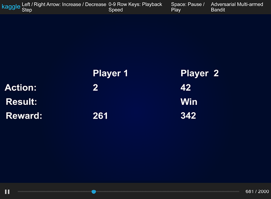
Figure 12.5: Snapshot from a rendered environment evaluating agent performance

In this section, we demonstrated how a vintage multi-armed bandit algorithm can be utilized in a simulation competition on Kaggle. While useful as a starting point, this was not sufficient to qualify for the medal zone, where deep reinforcement learning approaches were more popular.

We will follow up with a discussion of approaches based on other methods, in a diverse range of competitions.

The name of the game

Beyond the relatively elementary games discussed above, simulation competitions involve more elaborate setups. In this section, we will briefly discuss those. The first example is Halite, defined on the competition page (https://www.kaggle.com/c/halite) in the following manner:

Halite [...] is a resource management game where you build and control a small armada of ships. Your algorithms determine their movements to collect halite, a luminous energy source. The most halite at the end of the match wins, but it’s up to you to figure out how to make effective and efficient moves. You control your fleet, build new ships, create shipyards, and mine the regenerating halite on the game board.

This is what the game looks like:

Figure 12.6: Halite game board

Kaggle organized two competitions around the game: a Playground edition (https://www.kaggle.com/c/halite-iv-playground-edition) as well as a regular Featured edition (https://www.kaggle.com/c/halite). The classic reinforcement learning approach was less useful in this instance since, with an arbitrary number of units (ships/bases) and a dynamic opponent pool, the problem of credit assignment was becoming intractable for people with access to a “normal” level of computing resources.

A description of the winning solution by Tom van de Wiele (https://www.kaggle.com/c/halite/discussion/183543) provides an excellent overview of the modified approach that proved successful in this instance (deep RL with independent credit assignment per unit).

Another competition involving a relatively sophisticated game was Lux AI (https://www.kaggle.com/c/lux-ai-2021). In this competition, participants were tasked with designing agents to tackle a multi-variable optimization problem combining resource gathering and allocation, competing against other players. In addition, successful agents had to analyze the moves of their opponents and react accordingly. An interesting feature of this contest was the popularity of a “meta” approach: imitation learning (https://paperswithcode.com/task/imitation-learning). This is a fairly novel approach in RL, focused on learning a behavior policy from demonstration – without a specific model to describe the generation of state-action pairs. A competitive implementation of this idea (at the time of writing) is given by Kaggle user Ironbar (https://www.kaggle.com/c/lux-ai-2021/discussion/293911).

Finally, no discussion of simulation competitions in Kaggle would be complete without the Google Research Football with Manchester City F.C. competition (https://www.kaggle.com/c/google-football/overview). The motivation behind this contest was for researchers to explore AI agents’ ability to play in complex settings like football. The competition Overview section formulates the problem thus:

The sport requires a balance of short-term control, learned concepts such as passing, and high-level strategy, which can be difficult to teach agents. A current environment exists to train and test agents, but other solutions may offer better results.

Unlike some examples given above, this competition was dominated by reinforcement learning approaches:

• Team Raw Beast (3^rd) followed a methodology inspired by AlphaStar: https://www.kaggle.com/c/google-football/discussion/200709
• Salty Fish (2^nd) utilized a form of self-play: https://www.kaggle.com/c/google-football/discussion/202977
• The winners, WeKick, used a deep learning-based solution with creative feature engineering and reward structure adjustment: https://www.kaggle.com/c/google-football/discussion/202232

Studying the solutions listed above is an excellent starting point to learn how RL can be utilized to solve this class of problems.

Firat Gonen

https://www.kaggle.com/frtgnn

For this chapter’s interview, we spoke to Firat Gonen, a Triple Grandmaster in Datasets, Notebooks, and Discussion, and an HP Data Science Global Ambassador. He gives us his take on his Kaggle approach, and how his attitude has evolved over time.

What’s your favorite kind of competition and why? In terms of technique and solving approaches, what is your specialty on Kaggle?

My favorite kind evolved over time. I used to prefer very generic tabular competitions where a nice laptop and some patience would suffice to master the trends. I felt like I used to be able to see the outlying trends between training and test sets pretty good. Over time, with being awarded the ambassadorship by Z by HP and my workstation equipment, I kind of converted myself towards more computer vision competitions, though I still have a lot to learn.

How do you approach a Kaggle competition? How different is this approach to what you do in your day-to-day work?

I usually prefer to delay the modeling part for as long as I can. I like to use that time on EDAs, outliers, reading the forum, etc., trying to be patient. After I feel like I’m done with feature engineering, I try to form only benchmark models to get a grip on different architecture results. My technique is very similar when it comes to professional work as well. I find it useless to try to do the best in a huge amount of time; there has to be a balance between time and success.

Tell us about a particularly challenging competition you entered, and what insights you used to tackle the task.

The competition hosted by François Chollet was extremely challenging; the very first competition to force us into AGI. I remember I felt pretty powerless in that competition, where I learned several new techniques. I think everybody did that while remembering data science is not just machine learning. Several other techniques like mixed integer programming resurfaced at Kaggle.

Has Kaggle helped you in your career? If so, how?

Of course: I learned a lot of new techniques and stayed up to date thanks to Kaggle. I’m in a place in my career where my main responsibility lies mostly in management. That’s why Kaggle is very important to me for staying up to date in several things.

How have you built up your portfolio thanks to Kaggle?

I believe the advantage was in a more indirect way, where people saw both practical skills (thanks to Kaggle) and more theoretical skills in my more conventional education qualifications.

In your experience, what do inexperienced Kagglers often overlook? What do you know now that you wish you’d known when you first started?

I think there are two things newcomers do wrong. The first one is having fear in entering a new competition, thinking that they will get bad scores and it will be registered. This is nonsense. Everybody has bad scores; it’s all about how much you devote to a new competition. The second one is that they want to get to the model-building stage ASAP, which is very wrong; they want to see their benchmark scores and then they get frustrated. I advise them to take their time in feature generation and selection, and also in EDA stages.

What mistakes have you made in competitions in the past?

My mistakes are, unfortunately, very similar to new rookies. I got impatient in several competitions where I didn’t pay enough attention to early stages, and after some time you feel like you don’t have enough time to go back.

Are there any particular tools or libraries that you would recommend using for data analysis or machine learning?

I would recommend PyCaret for benchmarking to get you speed, and PyTorch for a model-building framework.

What’s the most important thing someone should keep in mind or do when they’re entering a competition?

Exploratory data analysis and previous similar competition discussions.

Do you use other competition platforms? How do they compare to Kaggle?

To be honest, I haven’t rolled the dice outside Kaggle, but I have had my share of them from a tourist perspective. It takes time to adjust to other platforms.

Summary

In this chapter, we discussed simulation competitions, a new type of contest that is increasing in popularity. Compared to vision or NLP-centered ones, simulation contests involve a much broader range of methods (with somewhat higher mathematical content), which reflects the difference between supervised learning and reinforcement learning.

This chapter concludes the technical part of the book. In the remainder, we will talk about turning your Kaggle Notebooks into a portfolio of projects and capitalizing on it to find new professional opportunities.

Join our book’s Discord space

Join the book’s Discord workspace for a monthly Ask me Anything session with the authors:

https://packt.link/KaggleDiscord