
10
Modeling for Computer Vision
Computer vision tasks are among the most popular problems in practical applications of machine learning; they were the gateway into deep learning for many Kagglers, including yours truly (Konrad, that is). Over the last few years, there has been tremendous progress in the field and new SOTA libraries continue to be released. In this chapter, we will give you an overview of the most popular competition types in computer vision:
- Image classification
- Object detection
- Image segmentation
We will begin with a short section on image augmentation, a group of task-agnostic techniques that can be applied to different problems to increase the generalization capability of our models.
Augmentation strategies
While deep learning techniques have been extremely successful in computer vision tasks like image recognition, segmentation, or object detection, the underlying algorithms are typically extremely data-intensive: they require large amounts of data to avoid overfitting. However, not all domains of interest satisfy that requirement, which is where data augmentation comes in. This is the name for a group of image processing techniques that create modified versions of images, thus enhancing the size and quality of training datasets, leading to better performance of deep learning models. The augmented data will typically represent a more comprehensive set of possible data points, thereby minimizing the distance between the training and validation set, as well as any future test sets.
In this section, we will review some of the more common augmentation techniques, along with choices for their software implementations. The most frequently used transformations include:
- Flipping: Flipping the image (along the horizontal or vertical axis)
- Rotation: Rotating the image by a given angle (clockwise or anti-clockwise)
- Cropping: A random subsection of the image is selected
- Brightness: Modifying the brightness of the image
- Scaling: The image is increased or decreased to a higher (outward) or lower (inward) size
Below, we demonstrate how those transformations work in practice using the image of an American acting legend and comedian, Betty White:

Figure 10.1: Betty White image
We can flip the image along the vertical or horizontal axes:
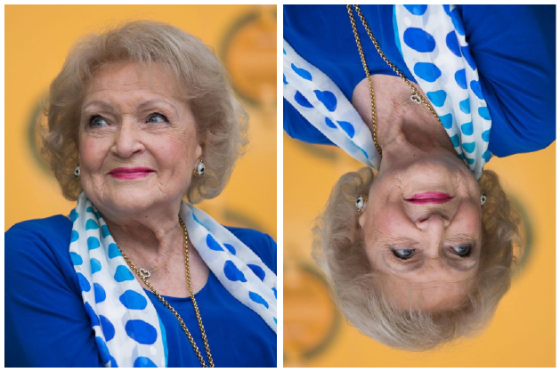
Figure 10.2: Betty White image – flipped vertically (left) and horizontally (right)
Rotations are fairly self-explanatory; notice the automatic padding of the image in the background:
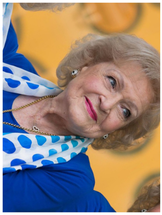
Figure 10.3: Betty White image – rotated clockwise
We can also crop an image to the region of interest:
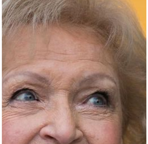
Figure 10.4: Betty White image – cropped
On a high level, we can say that augmentations can be applied in one of two ways:
- Offline: These are usually applied for smaller datasets (fewer images or smaller sizes, although the definition of “small” depends on the available hardware). The idea is to generate modified versions of the original images as a preprocessing step for your dataset, and then use those alongside the “original” ones.
- Online: These are used for bigger datasets. The augmented images are not saved on disk; the augmentations are applied in mini-batches and fed to the model.
In the next few sections, we will give you an overview of two of the most common methods for augmenting your image dataset: the built-in Keras functionality and the albumentations package. There are several other options available out there (skimage, OpenCV, imgaug, Augmentor, SOLT), but we will focus on the most popular ones.
The methods discussed in this chapter focus on image analysis powered by GPU. The use of tensor processing units (TPUs) is an emerging, but still somewhat niche, application. Readers interested in image augmentation in combination with TPU-powered analysis are encouraged to check out the excellent work of Chris Deotte (@cdeotte):
https://www.kaggle.com/cdeotte/triple-stratified-kfold-with-tfrecords
Chris is a quadruple Kaggle Grandmaster and a fantastic educator through the Notebooks he creates and discussions he participates in; overall, a person definitely worth following for any Kaggler, irrespective of your level of experience.
We will be using data from the Cassava Leaf Disease Classification competition (https://www.kaggle.com/c/cassava-leaf-disease-classification). As usual, we begin with the groundwork: first, loading the necessary packages:
import os
import glob
import numpy as np
import scipy as sp
import pandas as pd
import cv2
from skimage.io import imshow, imread, imsave
# imgaug
import imageio
import imgaug as ia
import imgaug.augmenters as iaa
# Albumentations
import albumentations as A
# Keras
# from keras.preprocessing.image import ImageDataGenerator, array_to_img, img_to_array, load_img
# Visualization
import matplotlib.pyplot as plt
import matplotlib.image as mpimg
%matplotlib inline
import seaborn as sns
from IPython.display import HTML, Image
# Warnings
import warnings
warnings.filterwarnings("ignore")
Next, we define some helper functions that will streamline the presentation later. We need a way to load images into arrays:
def load_image(image_id):
    file_path = image_id
    image = imread(Image_Data_Path + file_path)
    return image
We would like to display multiple images in a gallery style, so we create a function that takes as input an array containing the images along with the desired number of columns, and outputs the array reshaped into a grid with a given number of columns:
def gallery(array, ncols=3):
    nindex, height, width, intensity = array.shape
    nrows = nindex//ncols
    assert nindex == nrows*ncols
    result = (array.reshape(nrows, ncols, height, width, intensity)
              .swapaxes(1,2)
              .reshape(height*nrows, width*ncols, intensity))
    return result
With the boilerplate taken care of, we can load the images for augmentation:
data_dir = '../input/cassava-leaf-disease-classification/'
Image_Data_Path = data_dir + '/train_images/'
train_data = pd.read_csv(data_dir + '/train.csv')
# We load and store the first 10 images in memory for faster access
train_images = train_data["image_id"][:10].apply(load_image)
Let’s load a single image so we know what our reference is:
curr_img = train_images[7]
plt.figure(figsize = (15,15))
plt.imshow(curr_img)
plt.axis('off')
Here it is:
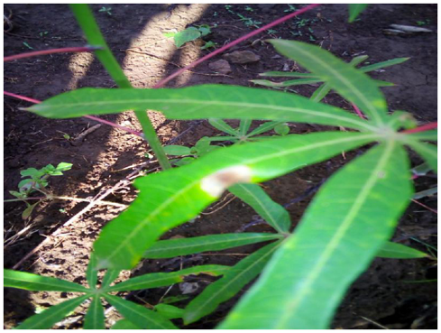
Figure 10.5: Reference image
In the following sections, we will demonstrate how to generate augmented images from this reference image using both built-in Keras functionality and the albumentations library.
Keras built-in augmentations
The Keras library has a built-in functionality for augmentations. While not as extensive as dedicated packages, it has the advantage of easy integration with your code. We do not need a separate code block for defining the augmentation transformations but can incorporate them inside ImageDataGenerator, a functionality we are likely to be using anyway.
The first Keras approach we examine is based upon the ImageDataGenerator class. As the name suggests, it can be used to generate batches of image data with real-time data augmentations.
ImageDataGenerator approach
We begin by instantiating an object of class ImageDataGenerator in the following manner:
import tensorflow as tf
from tensorflow.keras.preprocessing.image import ImageDataGenerator,
array_to_img, img_to_array, load_img
datagen = ImageDataGenerator(
        rotation_range = 40,
        shear_range = 0.2,
        zoom_range = 0.2,
        horizontal_flip = True,
        brightness_range = (0.5, 1.5))
curr_img_array = img_to_array(curr_img)
curr_img_array = curr_img_array.reshape((1,) + curr_img_array.shape)
We define the desired augmentations as arguments to ImageDataGenerator. The official documentation does not seem to address the topic, but practical results indicate that the augmentations are applied in the order in which they are defined as arguments.
In the above example, we utilize only a limited subset of possible options; for a full list, the reader is encouraged to consult the official documentation: https://keras.io/api/preprocessing/image/.
Next, we iterate through the images with the .flow method of the ImageDataGenerator object. The class provides three different functions to load the image dataset in memory and generate batches of augmented data:
flowflow_from_directoryflow_from_dataframe
They all achieve the same objective, but differ in the way the locations of the files are specified. In our example, the images are already in memory, so we can iterate using the simplest method:
i = 0
for batch in datagen.flow(
    curr_img_array,
    batch_size=1,
    save_to_dir='.',
    save_prefix='Augmented_image',
    save_format='jpeg'):
    i += 1
    # Hard-coded stop - without it, the generator enters an infinite loop
    if i > 9:
        break
We can examine the augmented images using the helper functions we defined earlier:
aug_images = []
for img_path in glob.glob("*.jpeg"):
    aug_images.append(mpimg.imread(img_path))
plt.figure(figsize=(20,20))
plt.axis('off')
plt.imshow(gallery(np.array(aug_images[0:9]), ncols = 3))
plt.title('Augmentation examples')
Here is the result:
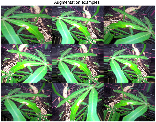
Figure 10.6: A collection of augmented images
Augmentations are a very useful tool, but using them efficiently requires a judgment call. First, it is obviously a good idea to visualize them to get a feeling for the impact on the data. On the one hand, we want to introduce some variation in the data to increase the generalization of our model; on the other, if we change the images too radically, the input data will be less informative and the model performance is likely to suffer. In addition, the choice of which augmentations to use can also be problem-specific, as we can see by comparing different competitions.
If you look at Figure 10.6 above (the reference image from the Cassava Leaf Disease Classification competition), the leaves on which we are supposed to identify the disease can be of different sizes, pointing at different angles, and so on, due both to the shapes of the plants and differences in how the images are taken. This means transformations such as vertical or horizontal flips, cropping, and rotations all make sense in this context.
By contrast, we can look at a sample image from the Severstal: Steel Defect Detection competition (https://www.kaggle.com/c/severstal-steel-defect-detection). In this competition, participants had to localize and classify defects on a steel sheet. All the images had the same size and orientation, which means that rotations or crops would have produced unrealistic images, adding to the noise and having an adverse impact on the generalization capabilities of an algorithm.
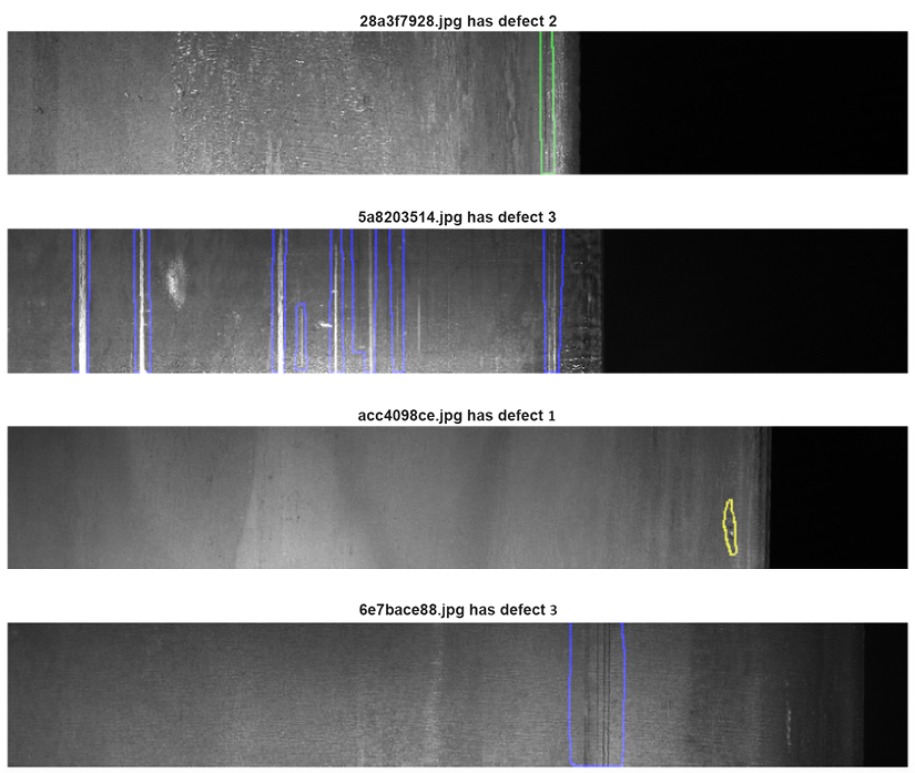
Figure 10.7: Sample images from the Severstal competition
Preprocessing layers
An alternative approach to data augmentation as a preprocessing step in a native Keras manner is to use the preprocessing layers API. The functionality is remarkably flexible: these pipelines can be used either in combination with Keras models or independently, in a manner similar to ImageDataGenerator.
Below we show briefly how a preprocessing layer can be set up. First, the imports:
from tensorflow.keras.layers.experimental import preprocessing
from tensorflow.keras import layers
We load a pretrained model in the standard Keras manner:
pretrained_base = tf.keras.models.load_model(
    '../input/cv-course-models/cv-course-models/vgg16-pretrained-base',
)
pretrained_base.trainable = False
The preprocessing layers can be used in the same way as other layers are used inside the Sequential constructor; the only requirement is that they need to be specified before any others, at the beginning of our model definition:
model = tf.keras.Sequential([
    # Preprocessing layers
    preprocessing.RandomFlip('horizontal'), # Flip left-to-right
    preprocessing.RandomContrast(0.5), # Contrast change by up to 50%
    # Base model
    pretrained_base,
    # model head definition
    layers.Flatten(),
    layers.Dense(6, activation='relu'),
    layers.Dense(1, activation='sigmoid'),
])
albumentations
The albumentations package is a fast image augmentation library that is built as a wrapper of sorts around other libraries.
The package is the result of intensive coding in quite a few Kaggle competitions (see https://medium.com/@iglovikov/the-birth-of-albumentations-fe38c1411cb3), and claims among its core developers and contributors quite a few notable Kagglers, including Eugene Khvedchenya (https://www.kaggle.com/bloodaxe), Vladimir Iglovikov (https://www.kaggle.com/iglovikov), Alex Parinov (https://www.kaggle.com/creafz), and ZFTurbo (https://www.kaggle.com/zfturbo).
The full documentation can be found at https://albumentations.readthedocs.io/en/latest/.
Below we list the important characteristics:
- A unified API for different data types
- Support for all common computer vision tasks
- Integration both with TensorFlow and PyTorch
Using albumentations functionality to transform an image is straightforward. We begin by initializing the required transformations:
import albumentations as A
horizontal_flip = A.HorizontalFlip(p=1)
rotate = A.ShiftScaleRotate(p=1)
gaus_noise = A.GaussNoise()
bright_contrast = A.RandomBrightnessContrast(p=1)
gamma = A.RandomGamma(p=1)
blur = A.Blur()
Next, we apply the transformations to our reference image:
img_flip = horizontal_flip(image = curr_img)
img_gaus = gaus_noise(image = curr_img)
img_rotate = rotate(image = curr_img)
img_bc = bright_contrast(image = curr_img)
img_gamma = gamma(image = curr_img)
img_blur = blur(image = curr_img)
We can access the augmented images with the 'image' key and visualize the results:
img_list = [img_flip['image'],img_gaus['image'], img_rotate['image'],
            img_bc['image'], img_gamma['image'], img_blur['image']]
plt.figure(figsize=(20,20))
plt.axis('off')
plt.imshow(gallery(np.array(img_list), ncols = 3))
plt.title('Augmentation examples')
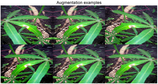
Figure 10.8: Image augmented using the albumentations library
Having discussed augmentation as a crucial preprocessing step in approaching a computer vision problem, we are now in a position to apply this knowledge in the following sections, beginning with a very common task: image classification.

Chris Deotte
https://www.kaggle.com/cdeotte
Before we proceed, let’s look at a brief conversation we had with Chris Deotte, who we’ve mentioned quite a few times in this book (including earlier in this chapter), and for good reason. He is a quadruple Kaggle Grandmaster and Senior Data Scientist & Researcher at NVIDIA, who joined Kaggle in 2019.
What’s your favorite kind of competition and why? In terms of techniques and solving approaches, what is your specialty on Kaggle?
I enjoy competitions with fascinating data and competitions that require building creative novel models. My specialty is analyzing trained models to determine their strengths and weaknesses. Afterward, I enjoy improving the models and/or developing post-processing to boost CV LB.
How do you approach a Kaggle competition? How different is this approach to what you do in your day-to-day work?
I begin each competition by performing EDA (exploratory data analysis), creating a local validation, building some simple models, and submitting to Kaggle for leaderboard scores. This fosters an intuition of what needs to be done in order to build an accurate and competitive model.
Tell us about a particularly challenging competition you entered, and what insights you used to tackle the task.
Kaggle’s Shopee – Price Match Guarantee was a challenging competition that required both image models and natural language models. A key insight was extracting embeddings from the two types of models and then determining how to use both image and language information together to find product matches.
Has Kaggle helped you in your career? If so, how?
Yes. Kaggle helped me become a senior data scientist at NVIDIA by improving my skills and boosting my resume’s marketability.
Many employers peruse the work on Kaggle to find employees with specific skills to help solve their specific projects. In this way, I have been solicited about many job opportunities.
In your experience, what do inexperienced Kagglers often overlook? What do you know now that you wish you’d known when you first started?
In my opinion, inexperienced Kagglers often overlook the importance of local validation. Seeing your name on the leaderboard is exciting. And it’s easy to focus on improving our leaderboard scores instead of our cross-validation scores.
What mistakes have you made in competitions in the past?
Many times, I have made the mistake of trusting my leaderboard score over my cross-validation score and selecting the wrong final submission.
Are there any particular tools or libraries that you would recommend using for data analysis or machine learning?
Absolutely. Feature engineering and quick experimentation are important when optimizing tabular data models. In order to accelerate the cycle of experimentation and validation, using NVIDIA RAPIDS cuDF and cuML on GPU are essential.
What’s the most important thing someone should keep in mind or do when they’re entering a competition?
The most important thing is to have fun and learn. Don’t worry about your final placement. If you focus on learning and having fun, then over time your final placements will become better and better.
Do you use other competition platforms? How do they compare to Kaggle?
Yes, I have entered competitions outside of Kaggle. Individual companies like Booking.com or Twitter.com will occasionally host a competition. These competitions are fun and involve high-quality, real-life data.
Classification
In this section, we will demonstrate an end-to-end pipeline that can be used as a template for handling image classification problems. We will walk through the necessary steps, from data preparation, to model setup and estimation, to results visualization. Apart from being informative (and cool), this last step can also be very useful if you need to examine your code in-depth to get a better understanding of the performance.
We will continue using the data from the Cassava Leaf Disease Classification contest (https://www.kaggle.com/c/cassava-leaf-disease-classification).
As usual, we begin by loading the necessary libraries:
import numpy as np
import pandas as pd
import matplotlib.pyplot as plt
import datetime
from sklearn.model_selection import train_test_split
from sklearn.metrics import accuracy_score
import tensorflow as tf
from tensorflow.keras import models, layers
from tensorflow.keras.preprocessing import image
from tensorflow.keras.preprocessing.image import ImageDataGenerator
from tensorflow.keras.callbacks import ModelCheckpoint, EarlyStopping, ReduceLROnPlateau
from tensorflow.keras.applications import EfficientNetB0
from tensorflow.keras.optimizers import Adam
import os, cv2, json
from PIL import Image
It is usually a good idea to define a few helper functions; it makes for code that is easier to both read and debug. If you are approaching a general image classification problem, a good starting point can be provided by a model from the EfficientNet family, introduced in 2019 in a paper from the Google Research Brain Team (https://arxiv.org/abs/1905.11946). The basic idea is to balance network depth, width, and resolution to enable more efficient scaling across all dimensions and subsequently better performance. For our solution, we will use the simplest member of the family, EfficientNet B0, which is a mobile-sized network with 11 million trainable parameters.
For a properly detailed explanation of the EfficientNet networks, you are encouraged to explore https://ai.googleblog.com/2019/05/efficientnet-improving-accuracy-and.html as a starting point.
We construct our model with B0 as the basis, followed by a pooling layer for improved translation invariance and a dense layer with an activation function suitable for our multiclass classification problem:
class CFG:
    # config
    WORK_DIR = '../input/cassava-leaf-disease-classification'
    BATCH_SIZE = 8
    EPOCHS = 5
    TARGET_SIZE = 512
def create_model():
    conv_base = EfficientNetB0(include_top = False, weights = None,
                               input_shape = (CFG.TARGET_SIZE,
                               CFG.TARGET_SIZE, 3))
    model = conv_base.output
    model = layers.GlobalAveragePooling2D()(model)
    model = layers.Dense(5, activation = "softmax")(model)
    model = models.Model(conv_base.input, model)
    model.compile(optimizer = Adam(lr = 0.001),
                  loss = "sparse_categorical_crossentropy",
                  metrics = ["acc"])
    return model
Some brief remarks on the parameters we pass to the EfficientNetB0 function:
- The
include_topparameter allows you to decide whether to include the final dense layers. As we want to use the pre-trained model as a feature extractor, a default strategy would be to skip them and then define the head ourselves. weightscan be set toNoneif we want to train the model from scratch, or to'imagenet'or'noisy-student'if we instead prefer to utilize the weights pre-trained on large image collections.
The helper function below allows us to visualize the activation layer, so we can examine the network performance from a visual angle. This is frequently helpful in developing an intuition in a field notorious for its opacity:
def activation_layer_vis(img, activation_layer = 0, layers = 10):
    layer_outputs = [layer.output for layer in model.layers[:layers]]
    activation_model = models.Model(inputs = model.input,
                                    outputs = layer_outputs)
    activations = activation_model.predict(img)

    rows = int(activations[activation_layer].shape[3] / 3)
    cols = int(activations[activation_layer].shape[3] / rows)
    fig, axes = plt.subplots(rows, cols, figsize = (15, 15 * cols))
    axes = axes.flatten()

    for i, ax in zip(range(activations[activation_layer].shape[3]), axes):
        ax.matshow(activations[activation_layer][0, :, :, i],
                   cmap = 'viridis')
        ax.axis('off')
    plt.tight_layout()
    plt.show()
We generate the activations by creating predictions for a given model based on a “restricted” model, in other words, using the entire architecture up until the penultimate layer; this is the code up to the activations variable. The rest of the function ensures we show the right layout of activations, corresponding to the shape of the filter in the appropriate convolution layer.
Next, we process the labels and set up the validation scheme; there is no special structure in the data (for example, a time dimension or overlap across classes), so we can use a simple random split:
train_labels = pd.read_csv(os.path.join(CFG.WORK_DIR, "train.csv"))
STEPS_PER_EPOCH = len(train_labels)*0.8 / CFG.BATCH_SIZE
VALIDATION_STEPS = len(train_labels)*0.2 / CFG.BATCH_SIZE
For a refresher on more elaborate validation schemes, refer to Chapter 6, Designing Good Validation.
We are now able to set up the data generators, which are necessary for our TF-based algorithm to loop through the image data.
First, we instantiate two ImageDataGenerator objects; this is when we incorporate the image augmentations. For the purpose of this demonstration, we will go with the Keras built-in ones. After that, we create the generator using a flow_from_dataframe() method, which is used to generate batches of tensor image data with real-time data augmentation:
train_labels.label = train_labels.label.astype('str')
train_datagen = ImageDataGenerator(
    validation_split = 0.2, preprocessing_function = None,
        rotation_range = 45, zoom_range = 0.2,
        horizontal_flip = True, vertical_flip = True,
        fill_mode = 'nearest', shear_range = 0.1,
        height_shift_range = 0.1, width_shift_range = 0.1)
train_generator = train_datagen.flow_from_dataframe(
    train_labels,
    directory = os.path.join(CFG.WORK_DIR, "train_images"),
    subset = "training",
    x_col = "image_id",y_col = "label",
    target_size = (CFG.TARGET_SIZE, CFG.TARGET_SIZE),
    batch_size = CFG.BATCH_SIZE,
    class_mode = "sparse")
validation_datagen = ImageDataGenerator(validation_split = 0.2)
validation_generator = validation_datagen.flow_from_dataframe(
        train_labels,
        directory = os.path.join(CFG.WORK_DIR, "train_images"),
        subset = "validation",
        x_col = "image_id",y_col = "label",
        target_size = (CFG.TARGET_SIZE, CFG.TARGET_SIZE),
        batch_size = CFG.BATCH_SIZE, class_mode = "sparse")
With the data structures specified, we can create the model:
model = create_model()
model.summary()
Once our model is created, we can quickly examine a summary. This is mostly useful for sanity checks, because unless you have a photographic memory, chances are you are not going to remember the layer composition batches of a sophisticated model like EffNetB0. In practice, you can use the summary to check whether the dimensions of output filters are correct or whether the parameter counts (trainable on non-trainable) are in line with expectations. For the sake of compactness, we only demonstrate the first few lines of the output below; inspecting the architecture diagram for B0 will give you an idea of how long the complete output would be.
Model: "functional_1"
__________________________________________________________________________
Layer (type)                  Output Shape         Param # Connected to
==========================================================================
input_1 (InputLayer)          [(None, 512, 512, 3) 0
__________________________________________________________________________
rescaling (Rescaling)         (None, 512, 512, 3)  0       input_1[0][0]
__________________________________________________________________________
normalization (Normalization) (None, 512, 512, 3)  7       rescaling[0][0]
___________________________________________________________________________
stem_conv_pad (ZeroPadding2D) (None, 513, 513, 3)  0       normalization[0][0]
___________________________________________________________________________
stem_conv (Conv2D)              (None, 256, 256, 32) 864    stem_conv_pad[0][0]
___________________________________________________________________________
stem_bn (BatchNormalization)    (None, 256, 256, 32) 128    stem_conv[0][0]
___________________________________________________________________________
stem_activation (Activation)    (None, 256, 256, 32) 0      stem_bn[0][0]
___________________________________________________________________________
block1a_dwconv (DepthwiseConv2D (None, 256, 256, 32) 288    stem_activation[0][0]
___________________________________________________________________________
block1a_bn (BatchNormalization) (None, 256, 256, 32) 128    block1a_dwconv[0][0]
___________________________________________________________________________
With the above steps taken care of, we can proceed to fitting the model. In this step, we can also very conveniently define callbacks. The first one is ModelCheckpoint:
model_save = ModelCheckpoint('./EffNetB0_512_8_best_weights.h5',
                             save_best_only = True,
                             save_weights_only = True,
                             monitor = 'val_loss',
                             mode = 'min', verbose = 1)
The checkpoint uses a few parameters worth elaborating on:
- We can preserve the best set of model weights by setting
save_best_only = True. - We reduce the size of the model by only keeping the weights, instead of the complete set of optimizer state.
- We decide on which model is optimal by locating a minimum for validation loss.
Next, we use one of the popular methods for preventing overfitting, early stopping. We monitor the performance of the model on the holdout set and stop the algorithm if the metric stops improving for a given number of epochs, in this case 5:
early_stop = EarlyStopping(monitor = 'val_loss', min_delta = 0.001,
                           patience = 5, mode = 'min',
                           verbose = 1, restore_best_weights = True)
The ReduceLROnPlateau callback monitors the loss on the holdout set and if no improvement is seen for a patience number of epochs, the learning rate is reduced, in this case by a factor of 0.3. While not a universal solution, it can frequently help with convergence:
reduce_lr = ReduceLROnPlateau(monitor = 'val_loss', factor = 0.3,
                              patience = 2, min_delta = 0.001,
                              mode = 'min', verbose = 1)
We are now ready to fit the model:
history = model.fit(
    train_generator,
    steps_per_epoch = STEPS_PER_EPOCH,
    epochs = CFG.EPOCHS,
    validation_data = validation_generator,
    validation_steps = VALIDATION_STEPS,
    callbacks = [model_save, early_stop, reduce_lr]
)
We will briefly explain the two parameters we have not encountered before:
- The training generator yields
steps_per_epochbatches per training epoch. - When the epoch is finished, the validation generator produces
validation_stepsbatches.
An example output after calling model.fit() is given below:
Epoch 00001: val_loss improved from inf to 0.57514, saving model to ./EffNetB0_512_8_best_weights.h5
Once a model is fitted, we can examine the activations on a sample image using the helper function we wrote at the start. While this is not necessary for successful model execution, it can help determine what sort of features our model is extracting before applying the classification layer at the top:
activation_layer_vis(img_tensor, 0)
Here is what we might see:
Figure 10.9: Sample activations from a fitted model
We can generate the predictions with model.predict():
ss = pd.read_csv(os.path.join(CFG.WORK_DIR, "sample_submission.csv"))
preds = []
for image_id in ss.image_id:
    image = Image.open(os.path.join(CFG.WORK_DIR,  "test_images",
                                    image_id))
    image = image.resize((CFG.TARGET_SIZE, CFG.TARGET_SIZE))
    image = np.expand_dims(image, axis = 0)
    preds.append(np.argmax(model.predict(image)))
ss['label'] = preds
We build the predictions by iterating through the list of images. For each of them, we reshape the image to the required dimensions and pick the channel with the strongest signal (the model predicts class probabilities, of which we pick the largest one with argmax). The final predictions are class numbers, in line with the metric utilized in the competition.
We have now demonstrated a minimal end-to-end pipeline for image classification. Numerous improvements are, of course, possible – for instance, more augmentations, bigger architecture, callback customization – but the basic underlying template should provide you with a good starting point going forward.
We move on now to a second popular problem in computer vision: object detection.
Object detection
Object detection is a computer vision/image processing task where we need to identify instances of semantic objects of a certain class in an image or video. In classification problems like those discussed in the previous section, we simply need to assign a class to each image, whereas in object detection tasks, we want to draw a bounding box around an object of interest to locate it within an image.
In this section, we will use data from the Global Wheat Detection competition (https://www.kaggle.com/c/global-wheat-detection). In this competition, participants had to detect wheat heads, which are spikes atop plants containing grain. Detection of these in plant images is used to estimate the size and density of wheat heads across crop varieties. We will demonstrate how to train a model for solving this using Yolov5, a well-established model in object detection, and state-of-the-art until late 2021 when it was (based on preliminary results) surpassed by the YoloX architecture. Yolov5 gave rise to extremely competitive results in the competition and although it was eventually disallowed by the organizers due to licensing issues, it is very well suited for the purpose of this demonstration.
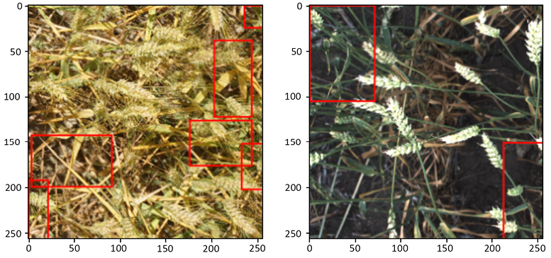
Figure 10.10: Sample image visualizations of detected wheat heads
An important point worth mentioning before we begin is the different formats for bounding box annotations; there are different (but mathematically equivalent) ways of describing the coordinates of a rectangle.
The most common types are coco, voc-pascal, and yolo. The differences between them are clear from the figure below:

Figure 10.11: Annotation formats for bounding boxes
One more part we need to define is the grid structure: Yolo detects objects by placing a grid over an image and checking for the presence of an object of interest (wheat head, in our case) in any of the cells. The bounding boxes are reshaped to be offset within the relevant cells of the image and the (x, y, w, h) parameters are scaled to the unit interval:

Figure 10.12: Yolo annotation positioning
We start by loading the annotations for our training data:
df = pd.read_csv('../input/global-wheat-detection/train.csv')
df.head(3)
Let’s inspect a few:
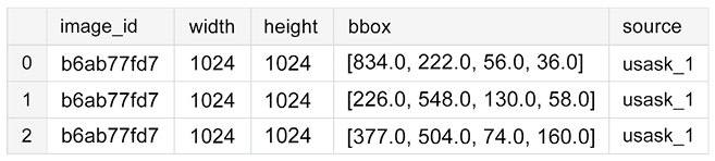
Figure 10.13: Training data with annotations
We extract the actual coordinates of the bounding boxes from the bbox column:
bboxs = np.stack(df['bbox'].apply(lambda x: np.fromstring(x[1:-1],
                                  sep=',')))
bboxs
Let’s look at the array:
array([[834., 222.,  56.,  36.],
       [226., 548., 130.,  58.],
       [377., 504.,  74., 160.],
       ...,
       [134., 228., 141.,  71.],
       [430.,  13., 184.,  79.],
       [875., 740.,  94.,  61.]])
The next step is to extract the coordinates in Yolo format into separate columns:
for i, column in enumerate(['x', 'y', 'w', 'h']):
    df[column] = bboxs[:,i]
df.drop(columns=['bbox'], inplace=True)
df['x_center'] = df['x'] + df['w']/2
df['y_center'] = df['y'] + df['h']/2
df['classes'] = 0
df = df[['image_id','x', 'y', 'w', 'h','x_center','y_center','classes']]
df.head(3)
The implementation from Ultralytics has some requirements on the structure of the dataset, specifically, where the annotations are stored and the folders for training/validation data.
The creation of the folders in the code below is fairly straightforward, but a more inquisitive reader is encouraged to consult the official documentation (https://github.com/ultralytics/yolov5/wiki/Train-Custom-Data):
# stratify on source
source = 'train'
# Pick a single fold for demonstration's sake
fold = 0
val_index = set(df[df['fold'] == fold]['image_id'])
# Loop through the bounding boxes per image
for name,mini in tqdm(df.groupby('image_id')):
    # Where to save the files
    if name in val_index:
        path2save = 'valid/'
    else:
        path2save = 'train/'
    # Storage path for labels
    if not os.path.exists('convertor/fold{}/labels/'.
                          format(fold)+path2save):
        os.makedirs('convertor/fold{}/labels/'.format(fold)+path2save)
    with open('convertor/fold{}/labels/'.format(fold)+path2save+name+".
              txt", 'w+') as f:
   # Normalize the coordinates in accordance with the Yolo format requirements
        row = mini[['classes','x_center','y_center','w','h']].
        astype(float).values
        row = row/1024
        row = row.astype(str)
        for j in range(len(row)):
            text = ' '.join(row[j])
            f.write(text)
            f.write("
")
    if not os.path.exists('convertor/fold{}/images/{}'.
                          format(fold,path2save)):
        os.makedirs('convertor/fold{}/images/{}'.format(fold,path2save))
    # No preprocessing needed for images => copy them as a batch
    sh.copy("../input/global-wheat-detection/{}/{}.jpg".
            format(source,name),
            'convertor/fold{}/images/{}/{}.jpg'.
            format(fold,path2save,name))
The next thing we do is install the Yolo package itself. If you are running this in a Kaggle Notebook or Colab, make sure to double-check GPU is enabled; Yolo installation will actually work without it, but you are likely to run into all sorts of timeouts and memory issues due to CPU versus GPU performance differences.
!git clone https://github.com/ultralytics/yolov5  && cd yolov5 &&
pip install -r requirements.txt
We omit the output, as it is rather extensive. The last bit of preparation needed is the YAML configuration file, where we specify the training and validation data locations and the number of classes. We are only interested in detecting wheat heads and not distinguishing between different types, so we have one class (its name is only provided for notational consistency and can be an arbitrary string in this instance):
yaml_text = """train: /kaggle/working/convertor/fold0/images/train/
            val: /kaggle/working/convertor/fold0/images/valid/
            nc: 1
            names: ['wheat']"""
with open("wheat.yaml", 'w') as f:
    f.write(yaml_text)
%cat wheat.yaml
With that, we can start training our model:
!python ./yolov5/train.py --img 512 --batch 2 --epochs 3 --workers 2 --data wheat.yaml --cfg "./yolov5/models/yolov5s.yaml" --name yolov5x_fold0 --cache
Unless you are used to launching things from the command line, the incantation above is positively cryptic, so let’s discuss its composition in some detail:
train.pyis the workhorse script for training a YoloV5 model, starting from pre-trained weights.--img 512means we want the original images (which, as you can see, we did not preprocess in any way) to be rescaled to 512x512. For a competitive result, you should use a higher resolution, but this code was executed in a Kaggle Notebook, which has certain limitations on resources.--batchrefers to the batch size in the training process.--epochs 3means we want to train the model for three epochs.--workers 2specifies the number of workers in the data loader. Increasing this number might help performance, but there is a known bug in version 6.0 (the most recent one available in the Kaggle Docker image, as of the time of this writing) when the number of workers is too high, even on a machine where more might be available.--data wheat.yamlis the file pointing to our data specification YAML file, defined above.--cfg "./yolov5/models/yolov5s.yaml"specifies the model architecture and the corresponding set of weights to be used for initialization. You can use the ones provided with the installation (check the official documentation for details), or you can customize your own and keep them in the same.yamlformat.--namespecifies where the resulting model is to be stored.
We break down the output of the training command below. First, the groundwork:
Downloading the pretrained weights, setting up Weights&Biases https://wandb.ai/site integration, GitHub sanity check.
Downloading https://ultralytics.com/assets/Arial.ttf to /root/.config/Ultralytics/Arial.ttf...
wandb: (1) Create a W&B account
wandb: (2) Use an existing W&B account
wandb: (3) Don't visualize my results
wandb: Enter your choice: (30 second timeout)
wandb: W&B disabled due to login timeout.
train: weights=yolov5/yolov5s.pt, cfg=./yolov5/models/yolov5s.yaml, data=wheat.yaml, hyp=yolov5/data/hyps/hyp.scratch-low.yaml, epochs=3, batch_size=2, imgsz=512, rect=False, resume=False, nosave=False, noval=False, noautoanchor=False, evolve=None, bucket=, cache=ram, image_weights=False, device=, multi_scale=False, single_cls=False, optimizer=SGD, sync_bn=False, workers=2, project=yolov5/runs/train, name=yolov5x_fold0, exist_ok=False, quad=False, cos_lr=False, label_smoothing=0.0, patience=100, freeze=[0], save_period=-1, local_rank=-1, entity=None, upload_dataset=False, bbox_interval=-1, artifact_alias=latest
github: up to date with https://github.com/ultralytics/yolov5
YOLOv5  v6.1-76-gc94736a torch 1.9.1 CUDA:0 (Tesla P100-PCIE-16GB, 16281MiB)
hyperparameters: lr0=0.01, lrf=0.01, momentum=0.937, weight_decay=0.0005, warmup_epochs=3.0, warmup_momentum=0.8, warmup_bias_lr=0.1, box=0.05, cls=0.5, cls_pw=1.0, obj=1.0, obj_pw=1.0, iou_t=0.2, anchor_t=4.0, fl_gamma=0.0, hsv_h=0.015, hsv_s=0.7, hsv_v=0.4, degrees=0.0, translate=0.1, scale=0.5, shear=0.0, perspective=0.0, flipud=0.0, fliplr=0.5, mosaic=1.0, mixup=0.0, copy_paste=0.0
Weights & Biases: run 'pip install wandb' to automatically track and visualize YOLOv5  runs (RECOMMENDED)
TensorBoard: Start with 'tensorboard --logdir yolov5/runs/train', view at http://localhost:6006/
Downloading https://github.com/ultralytics/yolov5/releases/download/v6.1/yolov5s.pt to yolov5/yolov5s.pt...
100%|██████████████████████████████████████| 14.1M/14.1M [00:00<00:00, 40.7MB/s]
v6.1-76-gc94736a torch 1.9.1 CUDA:0 (Tesla P100-PCIE-16GB, 16281MiB)
hyperparameters: lr0=0.01, lrf=0.01, momentum=0.937, weight_decay=0.0005, warmup_epochs=3.0, warmup_momentum=0.8, warmup_bias_lr=0.1, box=0.05, cls=0.5, cls_pw=1.0, obj=1.0, obj_pw=1.0, iou_t=0.2, anchor_t=4.0, fl_gamma=0.0, hsv_h=0.015, hsv_s=0.7, hsv_v=0.4, degrees=0.0, translate=0.1, scale=0.5, shear=0.0, perspective=0.0, flipud=0.0, fliplr=0.5, mosaic=1.0, mixup=0.0, copy_paste=0.0
Weights & Biases: run 'pip install wandb' to automatically track and visualize YOLOv5 runs (RECOMMENDED)
TensorBoard: Start with 'tensorboard --logdir yolov5/runs/train', view at http://localhost:6006/
Downloading https://github.com/ultralytics/yolov5/releases/download/v6.1/yolov5s.pt to yolov5/yolov5s.pt...
100%|██████████████████████████████████████| 14.1M/14.1M [00:00<00:00, 40.7MB/s]
Then comes the model. We see a summary of the architecture, the optimizer setup, and the augmentations used:
Overriding model.yaml nc=80 with nc=1
                 from  n    params  module                                  arguments
  0                -1  1    3520  models.common.Conv                      [3, 32, 6, 2, 2]
  1                -1  1    18560  models.common.Conv                      [32, 64, 3, 2]
  2                -1  1    18816  models.common.C3                        [64, 64, 1]
  3                -1  1    73984  models.common.Conv                      [64, 128, 3, 2]
  4                -1  2    115712  models.common.C3                        [128, 128, 2]
  5                -1  1    295424  models.common.Conv                      [128, 256, 3, 2]
  6                -1  3    625152  models.common.C3                        [256, 256, 3]
  7                -1  1   1180672  models.common.Conv                      [256, 512, 3, 2]
  8                -1  1   1182720  models.common.C3                        [512, 512, 1]
  9                -1  1    656896  models.common.SPPF                      [512, 512, 5]
 10                -1  1    131584  models.common.Conv                      [512, 256, 1, 1]
 11                -1  1         0  torch.nn.modules.upsampling.Upsample    [None, 2, 'nearest']
 12           [-1, 6]  1         0  models.common.Concat                    [1]
 13                -1  1    361984  models.common.C3                        [512, 256, 1, False]
 14                -1  1     33024  models.common.Conv                      [256, 128, 1, 1]
 15                -1  1         0  torch.nn.modules.upsampling.Upsample    [None, 2, 'nearest']
 16           [-1, 4]  1         0  models.common.Concat                    [1]
 17                -1  1     90880  models.common.C3                        [256, 128, 1, False]
 18                -1  1    147712  models.common.Conv                      [128, 128, 3, 2]
 19          [-1, 14]  1         0  models.common.Concat                    [1]
 20                -1  1    296448  models.common.C3                        [256, 256, 1, False]
 21                -1  1    590336  models.common.Conv                      [256, 256, 3, 2]
 22          [-1, 10]  1         0  models.common.Concat                    [1]
 23                -1  1   1182720  models.common.C3                        [512, 512, 1, False]
 24      [17, 20, 23]  1     16182  models.yolo.Detect                      [1, [[10, 13, 16, 30, 33, 23], [30, 61, 62, 45, 59, 119], [116, 90, 156, 198, 373, 326]], [128, 256, 512]]
YOLOv5s summary: 270 layers, 7022326 parameters, 7022326 gradients, 15.8 GFLOPs
Transferred 342/349 items from yolov5/yolov5s.pt
Scaled weight_decay = 0.0005
optimizer: SGD with parameter groups 57 weight (no decay), 60 weight, 60 bias
albumentations: Blur(always_apply=False, p=0.01, blur_limit=(3, 7)), MedianBlur(always_apply=False, p=0.01, blur_limit=(3, 7)), ToGray(always_apply=False, p=0.01), CLAHE(always_apply=False, p=0.01, clip_limit=(1, 4.0), tile_grid_size=(8, 8))
train: Scanning '/kaggle/working/convertor/fold0/labels/train' images and labels
train: New cache created: /kaggle/working/convertor/fold0/labels/train.cache
train: Caching images (0.0GB ram): 100%|██████████| 51/51 [00:00<00:00, 76.00it/
val: Scanning '/kaggle/working/convertor/fold0/labels/valid' images and labels..
val: New cache created: /kaggle/working/convertor/fold0/labels/valid.cache
val: Caching images (2.6GB ram): 100%|██████████| 3322/3322 [00:47<00:00, 70.51i
Plotting labels to yolov5/runs/train/yolov5x_fold0/labels.jpg...
AutoAnchor: 6.00 anchors/target, 0.997 Best Possible Recall (BPR). Current anchors are a good fit to dataset
Image sizes 512 train, 512 val
Using 2 dataloader workers
This is followed by the actual training log:
Starting training for 3 epochs...
     Epoch   gpu_mem       box       obj       cls    labels  img_size
       0/2    0.371G    0.1196   0.05478         0        14       512: 100%|███
               Class     Images     Labels          P          R     [email protected] mAP@WARNING: NMS time limit 0.120s exceeded
               Class     Images     Labels          P          R     [email protected] mAP@
                 all       3322     147409    0.00774     0.0523    0.00437   0.000952
     Epoch   gpu_mem       box       obj       cls    labels  img_size
       1/2    0.474G    0.1176   0.05625         0         5       512: 100%|███
               Class     Images     Labels          P          R     [email protected] mAP@WARNING: NMS time limit 0.120s exceeded
               Class     Images     Labels          P          R     [email protected] mAP@WARNING: NMS time limit 0.120s exceeded
               Class     Images     Labels          P          R     [email protected] mAP@
                 all       3322     147409    0.00914     0.0618    0.00493    0.00108
     Epoch   gpu_mem       box       obj       cls    labels  img_size
       2/2    0.474G    0.1146   0.06308         0        12       512: 100%|███
               Class     Images     Labels          P          R     [email protected] mAP@
                 all       3322     147409    0.00997     0.0674    0.00558    0.00123
3 epochs completed in 0.073 hours.
Optimizer stripped from yolov5/runs/train/yolov5x_fold0/weights/last.pt, 14.4MB
Optimizer stripped from yolov5/runs/train/yolov5x_fold0/weights/best.pt, 14.4MB
Validating yolov5/runs/train/yolov5x_fold0/weights/best.pt...
Fusing layers...
YOLOv5s summary: 213 layers, 7012822 parameters, 0 gradients, 15.8 GFLOPs
               Class     Images     Labels          P          R     [email protected] mAP@WARNING: NMS time limit 0.120s exceeded
               Class     Images     Labels          P          R     [email protected] mAP@WARNING: NMS time limit 0.120s exceeded
               Class     Images     Labels          P          R     [email protected] mAP@WARNING: NMS time limit 0.120s exceeded
               Class     Images     Labels          P          R     [email protected] mAP@WARNING: NMS time limit 0.120s exceeded
               Class     Images     Labels          P          R     [email protected] mAP@WARNING: NMS time limit 0.120s exceeded
               Class     Images     Labels          P          R     [email protected] mAP@WARNING: NMS time limit 0.120s exceeded
               Class     Images     Labels          P          R     [email protected] mAP@WARNING: NMS time limit 0.120s exceeded
               Class     Images     Labels          P          R     [email protected] mAP@WARNING: NMS time limit 0.120s exceeded
               Class     Images     Labels          P          R     [email protected] mAP@WARNING: NMS time limit 0.120s exceeded
               Class     Images     Labels          P          R     [email protected] mAP@WARNING: NMS time limit 0.120s exceeded
               Class     Images     Labels          P          R     [email protected] mAP@
                 all       3322     147409    0.00997     0.0673    0.00556    0.00122
Results saved to yolov5/runs/train/yolov5x_fold0
The results from both training and validation stages can be examined; they are stored in the yolov5 folder under ./yolov5/runs/train/yolov5x_fold0:
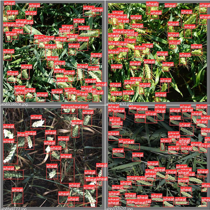
Figure 10.14: Validation data with annotations
Once we have trained the model, we can use the weights from the best performing model (Yolov5 has a neat functionality of automatically keeping both the best and last epoch model, storing them as best.pt and last.pt) to generate predictions on the test data:
!python ./yolov5/detect.py --weights ./yolov5/runs/train/yolov5x_fold0/weights/best.pt --img 512 --conf 0.1 --source /kaggle/input/global-wheat-detection/test --save-txt --save-conf --exist-ok
We will discuss the parameters that are specific to the inference stage:
--weightspoints to the location of the best weights from our model trained above.--conf 0.1specifies which candidate bounding boxes generated by the model should be kept. As usual, it is a compromise between precision and recall (too low a threshold gives a high number of false positives, while moving the threshold too high means we might not find any wheat heads at all).--sourceis the location of the test data.
The labels created for our test images can be inspected locally:
!ls ./yolov5/runs/detect/exp/labels/
This is what we might see:
2fd875eaa.txt  53f253011.txt  aac893a91.txt  f5a1f0358.txt
348a992bb.txt  796707dd7.txt  cc3532ff6.txt
Let’s look at an individual prediction:
!cat 2fd875eaa.txt
It has the following format:
0 0.527832 0.580566 0.202148 0.838867 0.101574
0 0.894531 0.587891 0.210938 0.316406 0.113519
This means that in image 2fd875eaa, our trained model detected two bounding boxes (their coordinates are entries 2-5 in the row), with confidence scores above 0.1 given at the end of the row.
How do we go about combining the predictions into a submission in the required format? We start by defining a helper function that helps us convert the coordinates from the yolo format to coco (as required in this competition): it is a matter of simple rearrangement of the order and normalizing to the original range of values by multiplying the fractions by the image size:
def convert(s):
    x = int(1024 * (s[1] - s[3]/2))
    y = int(1024 * (s[2] - s[4]/2))
    w = int(1024 * s[3])
    h = int(1024 * s[4])

    return(str(s[5]) + ' ' + str(x) + ' ' + str(y) + ' ' + str(w)
           + ' ' + str(h))
We then proceed to generate a submission file:
- We loop over the files listed above.
- For each file, all rows are converted into strings in the required format (one row represents one bounding box detected).
- The rows are then concatenated into a single string corresponding to this file.
The code is as follows:
with open('submission.csv', 'w') as myfile:
    # Prepare submission
    wfolder = './yolov5/runs/detect/exp/labels/'
    for f in os.listdir(wfolder):
        fname = wfolder + f
        xdat = pd.read_csv(fname, sep = ' ', header = None)
        outline = f[:-4] + ' ' + ' '.join(list(xdat.apply(lambda s:
                                     convert(s), axis = 1)))
        myfile.write(outline + '
')

myfile.close()
Let’s see what it looks like:
!cat submission.csv
53f253011 0.100472 61 669 961 57 0.106223 0 125 234 183 0.1082 96 696 928 126 0.108863 515 393 86 161 0.11459 31 0 167 209 0.120246 517 466 89 147
aac893a91 0.108037 376 435 325 188
796707dd7 0.235373 684 128 234 113
cc3532ff6 0.100443 406 752 144 108 0.102479 405 87 4 89 0.107173 576 537 138 94 0.113459 256 498 179 211 0.114847 836 618 186 65 0.121121 154 544 248 115 0.125105 40 567 483 199
2fd875eaa 0.101398 439 163 204 860 0.112546 807 440 216 323
348a992bb 0.100572 0 10 440 298 0.101236 344 445 401 211
f5a1f0358 0.102549 398 424 295 96
The generated submission.csv file completes our pipeline.
In this section, we have demonstrated how to use a YoloV5 to solve the problem of object detection: how to handle annotations in different formats, how to customize a model for a specific task, train it, and evaluate the results.
Based on this knowledge, you should be able to start working with object detection problems.
We now move on to the third popular class of computer vision tasks: semantic segmentation.
Semantic segmentation
The easiest way to think about segmentation is that it classifies each pixel in an image, assigning it to a corresponding class; combined, those pixels form areas of interest, such as regions with disease on an organ in medical images. By contrast, object detection (discussed in the previous section) classifies patches of an image into different object classes and creates bounding boxes around them.
We will demonstrate the modeling approach using data from the Sartorius – Cell Instance Segmentation competition (https://www.kaggle.com/c/sartorius-cell-instance-segmentation). In this one, the participants were tasked to train models for instance segmentation of neural cells using a set of microscopy images.
Our solution will be built around Detectron2, a library created by Facebook AI Research that supports multiple detection and segmentation algorithms.
Detectron2 is a successor to the original Detectron library (https://github.com/facebookresearch/Detectron/) and the Mask R-CNN project (https://github.com/facebookresearch/maskrcnn-benchmark/).
We begin by installing the extra packages:
!pip install pycocotools
!pip install 'git+https://github.com/facebookresearch/detectron2.git'
We install pycocotools (https://github.com/cocodataset/cocoapi/tree/master/PythonAPI/pycocotools), which we will need to format the annotations, and Detectron2 (https://github.com/facebookresearch/detectron2), our workhorse in this task.
Before we can train our model, we need a bit of preparation: the annotations need to be converted from the run-length encoding (RLE) format provided by the organizers to the COCO format required as input for Detectron2. The basic idea behind RLE is saving space: creating a segmentation means marking a group of pixels in a certain manner. Since an image can be thought of as an array, this area can be denoted by a series of straight lines (row- or column-wise).
You can encode each of those lines by listing the indices, or by specifying a starting position and the length of the subsequent contiguous block. A visual example is given below:
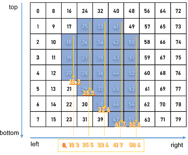
Figure 10.15: Visual representation of RLE
Microsoft’s Common Objects in Context (COCO) format is a specific JSON structure dictating how labels and metadata are saved for an image dataset. Below, we demonstrate how to convert RLE to COCO and combine it with a k-fold validation split, so we get the required train/validation pair of JSON files for each fold.
Let’s begin:
# from pycocotools.coco import COCO
import skimage.io as io
import matplotlib.pyplot as plt
from pathlib import Path
from PIL import Image
import pandas as pd
import numpy as np
from tqdm.notebook import tqdm
import json,itertools
from sklearn.model_selection import GroupKFold
# Config
class CFG:
    data_path = '../input/sartorius-cell-instance-segmentation/'
    nfolds = 5
We need three functions to go from RLE to COCO. First, we need to convert from RLE to a binary mask:
# From https://www.kaggle.com/stainsby/fast-tested-rle
def rle_decode(mask_rle, shape):
    '''
    mask_rle: run-length as string formatted (start length)
    shape: (height,width) of array to return
    Returns numpy array, 1 - mask, 0 - background
    '''
    s = mask_rle.split()
    starts, lengths = [np.asarray(x, dtype=int)
                       for x in (s[0:][::2], s[1:][::2])]
    starts -= 1
    ends = starts + lengths
    img = np.zeros(shape[0]*shape[1], dtype=np.uint8)
    for lo, hi in zip(starts, ends):
        img[lo:hi] = 1
    return img.reshape(shape)  # Needed to align to RLE direction
The second one converts a binary mask to RLE:
# From https://newbedev.com/encode-numpy-array-using-uncompressed-rle-for-
# coco-dataset
def binary_mask_to_rle(binary_mask):
    rle = {'counts': [], 'size': list(binary_mask.shape)}
    counts = rle.get('counts')
    for i, (value, elements) in enumerate(
            itertools.groupby(binary_mask.ravel(order='F'))):
        if i == 0 and value == 1:
            counts.append(0)
        counts.append(len(list(elements)))
    return rle
Finally, we combine the two in order to produce the COCO output:
def coco_structure(train_df):
    cat_ids = {name: id+1 for id, name in enumerate(
        train_df.cell_type.unique())}
    cats = [{'name': name, 'id': id} for name, id in cat_ids.items()]
    images = [{'id': id, 'width': row.width, 'height': row.height,
               'file_name':f'train/{id}.png'} for id,
               row in train_df.groupby('id').agg('first').iterrows()]
    annotations = []
    for idx, row in tqdm(train_df.iterrows()):
        mk = rle_decode(row.annotation, (row.height, row.width))
        ys, xs = np.where(mk)
        x1, x2 = min(xs), max(xs)
        y1, y2 = min(ys), max(ys)
        enc =binary_mask_to_rle(mk)
        seg = {
            'segmentation':enc,
            'bbox': [int(x1), int(y1), int(x2-x1+1), int(y2-y1+1)],
            'area': int(np.sum(mk)),
            'image_id':row.id,
            'category_id':cat_ids[row.cell_type],
            'iscrowd':0,
            'id':idx
        }
        annotations.append(seg)
    return {'categories':cats, 'images':images,'annotations':annotations}
We split our data into non-overlapping folds:
train_df = pd.read_csv(CFG.data_path + 'train.csv')
gkf = GroupKFold(n_splits = CFG.nfolds)
train_df["fold"] = -1
y = train_df.width.values
for f, (t_, v_) in enumerate(gkf.split(X=train_df, y=y,
                             groups=train_df.id.values)):
    train_df.loc[v_, "fold"] = f

fold_id = train_df.fold.copy()
We can now loop over the folds:
all_ids = train_df.id.unique()
# For fold in range(CFG.nfolds):
for fold in range(4,5):
    train_sample = train_df.loc[fold_id != fold]
    root = coco_structure(train_sample)
    with open('annotations_train_f' + str(fold) +
              '.json', 'w', encoding='utf-8') as f:
        json.dump(root, f, ensure_ascii=True, indent=4)

    valid_sample = train_df.loc[fold_id == fold]
    print('fold ' + str(fold) + ': produced')
for fold in range(4,5):
    train_sample = train_df.loc[fold_id == fold]
    root = coco_structure(train_sample)
    with open('annotations_valid_f' + str(fold) +
              '.json', 'w', encoding='utf-8') as f:
        json.dump(root, f, ensure_ascii=True, indent=4)

    valid_sample = train_df.loc[fold_id == fold]
    print('fold ' + str(fold) + ': produced')
The reason why the loop has to be executed in pieces is the size limit of the Kaggle environment: the maximum size of Notebook output is limited to 20 GB, and 5 folds with 2 files (training/validation) for each fold meant a total of 10 JSON files, exceeding that limit.
Such practical considerations are worth keeping in mind when running code in a Kaggle Notebook, although for such “preparatory” work, you can, of course, produce the results elsewhere, and upload them as Kaggle Datasets afterward.
With the splits produced, we can move toward training a Detectron2 model for our dataset. As usual, we start by loading the necessary packages:
from datetime import datetime
import os
import pandas as pd
import numpy as np
import pycocotools.mask as mask_util
import detectron2
from pathlib import Path
import random, cv2, os
import matplotlib.pyplot as plt
# Import some common detectron2 utilities
from detectron2 import model_zoo
from detectron2.engine import DefaultPredictor, DefaultTrainer
from detectron2.config import get_cfg
from detectron2.utils.visualizer import Visualizer, ColorMode
from detectron2.data import MetadataCatalog, DatasetCatalog
from detectron2.data.datasets import register_coco_instances
from detectron2.utils.logger import setup_logger
from detectron2.evaluation.evaluator import DatasetEvaluator
from detectron2.engine import BestCheckpointer
from detectron2.checkpoint import DetectionCheckpointer
setup_logger()
import torch
While the number of imports from Detectron2 can seem intimidating at first, their function will become clear as we progress with the task definition; we start by specifying paths to the input data folder, annotations folder, and a YAML file defining our preferred model architecture:
class CFG:
    wfold = 4
    data_folder = '../input/sartorius-cell-instance-segmentation/'
    anno_folder = '../input/sartoriusannotations/'
    model_arch = 'mask_rcnn_R_50_FPN_3x.yaml'
    nof_iters = 10000
    seed = 45
One point worth mentioning here is the iterations parameter (nof_iters above). Usually, model training is parametrized in terms of the number of epochs, in other words, complete passes through the training data. Detectron2 is engineered differently: one iteration refers to one mini-batch and different mini-batch sizes are used in different parts of the model.
In order to ensure the results are reproducible, we fix random seeds used by different components of the model:
def seed_everything(seed):
    random.seed(seed)
    os.environ['PYTHONHASHSEED'] = str(seed)
    np.random.seed(seed)
    torch.manual_seed(seed)
    torch.cuda.manual_seed(seed)
    torch.backends.cudnn.deterministic = True
seed_everything(CFG.seed)
The competition metric was the mean average precision at different intersection over union (IoU) thresholds. As a refresher from Chapter 5, Competition Tasks and Metrics, the IoU of a proposed set of object pixels and a set of true object pixels is calculated as:
![]()
The metric sweeps over a range of IoU thresholds, at each point calculating an average precision value. The threshold values range from 0.5 to 0.95, with increments of 0.05.
At each threshold value, a precision value is calculated based on the number of true positives (TP), false negatives (FN), and false positives (FP) resulting from comparing the predicted object with all ground truth objects. Lastly, the score returned by the competition metric is the mean taken over the individual average precisions of each image in the test dataset.
Below, we define the functions necessary to calculate the metric and use it directly inside the model as the objective function:
# Taken from https://www.kaggle.com/theoviel/competition-metric-map-iou
def precision_at(threshold, iou):
    matches = iou > threshold
    true_positives = np.sum(matches, axis=1) == 1  # Correct objects
    false_positives = np.sum(matches, axis=0) == 0  # Missed objects
    false_negatives = np.sum(matches, axis=1) == 0  # Extra objects
    return np.sum(true_positives), np.sum(false_positives),
    np.sum(false_negatives)
def score(pred, targ):
    pred_masks = pred['instances'].pred_masks.cpu().numpy()
    enc_preds = [mask_util.encode(np.asarray(p, order='F'))
                 for p in pred_masks]
    enc_targs = list(map(lambda x:x['segmentation'], targ))
    ious = mask_util.iou(enc_preds, enc_targs, [0]*len(enc_targs))
    prec = []
    for t in np.arange(0.5, 1.0, 0.05):
        tp, fp, fn = precision_at(t, ious)
        p = tp / (tp + fp + fn)
        prec.append(p)
    return np.mean(prec)
With the metric defined, we can use it in the model:
class MAPIOUEvaluator(DatasetEvaluator):
    def __init__(self, dataset_name):
        dataset_dicts = DatasetCatalog.get(dataset_name)
        self.annotations_cache = {item['image_id']:item['annotations']
                                  for item in dataset_dicts}

    def reset(self):
        self.scores = []
    def process(self, inputs, outputs):
        for inp, out in zip(inputs, outputs):
            if len(out['instances']) == 0:
                self.scores.append(0)
            else:
                targ = self.annotations_cache[inp['image_id']]
                self.scores.append(score(out, targ))
    def evaluate(self):
        return {"MaP IoU": np.mean(self.scores)}
This gives us the basis for creating a Trainer object, which is the workhorse of our solution built around Detectron2:
class Trainer(DefaultTrainer):
    @classmethod
    def build_evaluator(cls, cfg, dataset_name, output_folder=None):
        return MAPIOUEvaluator(dataset_name)
    def build_hooks(self):
        # copy of cfg
        cfg = self.cfg.clone()
        # build the original model hooks
        hooks = super().build_hooks()
        # add the best checkpointer hook
        hooks.insert(-1, BestCheckpointer(cfg.TEST.EVAL_PERIOD,
                                         DetectionCheckpointer(self.model,
                                         cfg.OUTPUT_DIR),
                                         "MaP IoU",
                                         "max",
                                         ))
        return hooks
We now proceed to load the training/validation data in Detectron2 style:
dataDir=Path(CFG.data_folder)
register_coco_instances('sartorius_train',{}, CFG.anno_folder +
                        'annotations_train_f' + str(CFG.wfold) +
                        '.json', dataDir)
register_coco_instances('sartorius_val',{}, CFG.anno_folder +
                        'annotations_valid_f' + str(CFG.wfold) +
                        '.json', dataDir)
metadata = MetadataCatalog.get('sartorius_train')
train_ds = DatasetCatalog.get('sartorius_train')
Before we instantiate a Detectron2 model, we need to take care of configuring it. Most of the values can be left at default values (at least, in a first pass); if you decide to tinker a bit more, start with BATCH_SIZE_PER_IMAGE (for increased generalization performance) and SCORE_THRESH_TEST (to limit false negatives):
cfg = get_cfg()
cfg.INPUT.MASK_FORMAT='bitmask'
cfg.merge_from_file(model_zoo.get_config_file('COCO-InstanceSegmentation/' +
                    CFG.model_arch))
cfg.DATASETS.TRAIN = ("sartorius_train",)
cfg.DATASETS.TEST = ("sartorius_val",)
cfg.DATALOADER.NUM_WORKERS = 2
cfg.MODEL.WEIGHTS = model_zoo.get_checkpoint_url('COCO-InstanceSegmentation/'
                    + CFG.model_arch)
cfg.SOLVER.IMS_PER_BATCH = 2
cfg.SOLVER.BASE_LR = 0.001
cfg.SOLVER.MAX_ITER = CFG.nof_iters
cfg.SOLVER.STEPS = []
cfg.MODEL.ROI_HEADS.BATCH_SIZE_PER_IMAGE = 512
cfg.MODEL.ROI_HEADS.NUM_CLASSES = 3
cfg.MODEL.ROI_HEADS.SCORE_THRESH_TEST = .4
cfg.TEST.EVAL_PERIOD = len(DatasetCatalog.get('sartorius_train'))
                           // cfg.SOLVER.IMS_PER_BATCH
Training a model is straightforward:
os.makedirs(cfg.OUTPUT_DIR, exist_ok=True)
trainer = Trainer(cfg)
trainer.resume_or_load(resume=False)
trainer.train()
You will notice that the output during training is rich in information about the progress of the procedure:
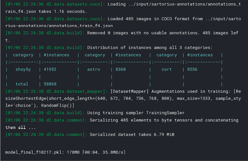
Figure 10.16: Training output from Detectron2
Once the model is trained, we can save the weights and use them for inference (potentially in a separate Notebook – see the discussion earlier in this chapter) and submission preparation. We start by adding new parameters that allow us to regularize the prediction, setting confidence thresholds and minimal mask sizes:
THRESHOLDS = [.18, .35, .58]
MIN_PIXELS = [75, 150, 75]
We need a helper function for encoding a single mask into RLE format:
def rle_encode(img):
    '''
    img: numpy array, 1 - mask, 0 - background
    Returns run length as string formatted
    '''
    pixels = img.flatten()
    pixels = np.concatenate([[0], pixels, [0]])
    runs = np.where(pixels[1:] != pixels[:-1])[0] + 1
    runs[1::2] -= runs[::2]
    return ' '.join(str(x) for x in runs)
Below is the main function for producing all masks per image, filtering out the dubious ones (with confidence scores below THRESHOLDS) with small areas (containing fewer pixels than MIN_PIXELS):
def get_masks(fn, predictor):
    im = cv2.imread(str(fn))
    pred = predictor(im)
    pred_class = torch.mode(pred['instances'].pred_classes)[0]
    take = pred['instances'].scores >= THRESHOLDS[pred_class]
    pred_masks = pred['instances'].pred_masks[take]
    pred_masks = pred_masks.cpu().numpy()
    res = []
    used = np.zeros(im.shape[:2], dtype=int)
    for mask in pred_masks:
        mask = mask * (1-used)
        # Skip predictions with small area
        if mask.sum() >= MIN_PIXELS[pred_class]:
            used += mask
            res.append(rle_encode(mask))
    return res
We then prepare the lists where image IDs and masks will be stored:
dataDir=Path(CFG.data_folder)
ids, masks=[],[]
test_names = (dataDir/'test').ls()
Competitions with large image sets – like the ones discussed in this section – often require training models for longer than 9 hours, which is the time limit imposed in Code competitions (see https://www.kaggle.com/docs/competitions). This means that training a model and running inference within the same Notebook becomes impossible. A typical workaround is to run a training Notebook/script first as a standalone Notebook in Kaggle, Google Colab, GCP, or locally. The output of this first Notebook (the trained weights) is used as input to the second one, in other words, to define the model used for predictions.
We proceed in that manner by loading the weights of our trained model:
cfg = get_cfg()
cfg.merge_from_file(model_zoo.get_config_file("COCO-InstanceSegmentation/"+
                    CFG.arch+".yaml"))
cfg.INPUT.MASK_FORMAT = 'bitmask'
cfg.MODEL.ROI_HEADS.NUM_CLASSES = 3
cfg.MODEL.WEIGHTS = CFG.model_folder + 'model_best_f' +
                    str(CFG.wfold)+'.pth'
cfg.MODEL.ROI_HEADS.SCORE_THRESH_TEST = 0.5
cfg.TEST.DETECTIONS_PER_IMAGE = 1000
predictor = DefaultPredictor(cfg)
We can visualize some of the predictions:
encoded_masks = get_masks(test_names[0], predictor)
_, axs = plt.subplots(1,2, figsize = (40, 15))
axs[1].imshow(cv2.imread(str(test_names[0])))
for enc in encoded_masks:
    dec = rle_decode(enc)
axs[0].imshow(np.ma.masked_where(dec == 0, dec))
Here is an example:
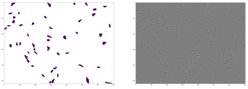
Figure 10.17: Visualizing a sample prediction from Detectron2 alongside the source image
With the helper functions defined above, producing the masks in RLE format for submission is straightforward:
for fn in test_names:
    encoded_masks = get_masks(fn, predictor)
    for enc in encoded_masks:
        ids.append(fn.stem)
        masks.append(enc)
pd.DataFrame({'id':ids, 'predicted':masks}).to_csv('submission.csv',
                                                   index=False)
pd.read_csv('submission.csv').head()
Here are the first few rows of the final submission:
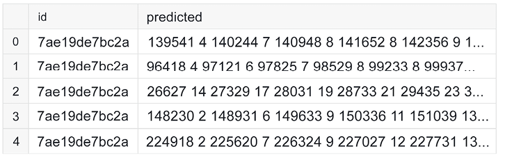
Figure 10.18: Formatted submission from a trained Detectron2 model
We have reached the end of the section. The pipeline above demonstrates how to set up a semantic segmentation model and train it. We have used a small number of iterations, but in order to achieve competitive results, longer training is necessary.

Laura Fink
https://www.kaggle.com/allunia
To wrap up this chapter, let’s see what Kaggler Laura Fink has to say about her time on the platform. As well as being a Notebooks Grandmaster and producing many masterful Notebooks, she is also Head of Data Science at MicroMata.
What’s your favorite kind of competition and why? In terms of techniques and solving approaches, what is your specialty on Kaggle?
My favorite competitions are those that want to yield something good to humanity. I especially like all healthcare-related challenges. Nonetheless, each competition feels like an adventure for me with its own puzzles to be solved. I really enjoy learning new skills and exploring new kinds of datasets or problems. Consequently, I’m not focused on specific techniques but rather on learning something new. I think I’m known for my strengths in exploratory data analysis (EDA).
How do you approach a Kaggle competition? How different is this approach to what you do in your day-to-day work?
When entering a competition, I start by reading the problem statement and the data description. After browsing through the forum and public Notebooks for collecting ideas, I usually start by developing my own solutions. In the initial phase, I spend some time on EDA to search for hidden groups and get some intuition. This helps quite a lot in setting up a proper validation strategy, which I believe is the foundation of all remaining steps. Then, I start to iterate through different parts of the machine learning pipeline like feature engineering or preprocessing, improving the model architecture, asking questions about the data collection, searching for leakages, doing more EDA, or building ensembles. I try to improve my solution in a greedy fashion. Kaggle competitions are very dynamic and one needs to try out diverse ideas and different solutions to survive in the end.
This is definitely different from my day-to-day work, where the focus is more on gaining insights from data and finding simple but effective solutions to improve business processes. Here, the task is often more complex than the models used. The problem to be solved has to be defined very clearly, which means that one has to discuss with experts of different backgrounds which goals should be reached, which processes are involved, and how the data needs to be collected or fused. Compared to Kaggle competitions, my daily work needs much more communication than machine learning skills.
Tell us about a particularly challenging competition you entered, and what insights you used to tackle the task.
The G2Net Gravitational Wave Detection competition was one of my favorites. The goal was to detect simulated gravitational wave signals that were hidden in noise originating from detector components and terrestrial forces. An important insight during this competition was that you should have a critical look at standard ways to analyze data and try out your own ideas. In the papers I read, the data was prepared mainly by using the Fourier or Constant-Q transform after whitening the data and applying a bandpass filter.
It came out very quickly that whitening was not helpful, as it used spline interpolation of the Power Spectral Density, which was itself very noisy. Fitting polynomials to small subsets of noisy data adds another source of errors because of overfitting.
After dropping the whitening, I tried out different hyperparameters of the Constant-Q transform, which turned out to be the leading method in the forum and public Notebooks for a long time. As there were two sources of gravitational waves that can be covered by different ranges of Q-values, I tried out an ensemble of models that differed in these hyperparameters. This turned out to be helpful in improving my score, but then I reached a limit. The Constant-Q transform applies a series of filters to time series and transforms them into the frequency domain. I started to ask myself if there was a method that does these filtering tasks in a better, more flexible way. It was at the same time that the idea of using 1 dim CNNs came up in the community, and I loved it. We all know that filters of 2 dim CNNs are able to detect edges, lines, and textures given image data. The same could be done with “classical” filters like the Laplace or Sobel filter. For this reason, I asked myself: can’t we use the 1dCNN to learn the most important filters on its own, instead of applying transformations that are already fixed somehow?
I was not able to get my 1 dim CNN solution to work, but it turned out that many top teams managed it well. The G2Net competition was one of my favorites even though I missed out on the goal of winning a medal. However, the knowledge I gained along the way and the lesson I learned about so-called standard approaches were very valuable.
Has Kaggle helped you in your career? If so, how?
I started my first job after university as a Java software developer even though I already had my first contact with machine learning during my master’s thesis. I was interested in doing more data analytics, but at that time, there were almost no data science jobs, or they were not named this way. When I heard about Kaggle the first time, I was trapped right from the start. Since then, I often found myself on Kaggle during the evenings to have some fun. It was not my intent to change my position at that time, but then a research project came up that needed machine learning skills. I was able to show that I was a suitable candidate for this project because of the knowledge I gained by participating on Kaggle. This turned out to be the entry point for my data science career.
Kaggle has always been a great place for me to try out ideas, learn new methods and tools, and gain practical experience. The skills I obtained this way have been quite helpful for data science projects at work. It’s like a boost of knowledge, as Kaggle provides a sandbox for you to try out different ideas and to be creative without risk. Failing in a competition means that there was at least one lesson to learn, but failing in a project can have a huge negative impact on yourself and other people.
Besides taking part in competitions, another great way to build up your portfolio is to write Notebooks. In doing so, you can show the world how you approach problems and how to communicate insights and conclusions. The latter is very important when you have to work with management, clients, and experts from different backgrounds.
In your experience, what do inexperienced Kagglers often overlook? What do you know now that you wish you’d known when you first started?
I think many beginners that enter competitions are seduced by the public leaderboard and build their models without having a good validation strategy. While measuring their success on the leaderboard, they are likely overfitting to the public test data. After the end of the competition, their models are not able to generalize to the unseen private test data, and they often fall down hundreds of places. I still remember how frustrated I was during the Mercedes-Benz Greener Manufacturing competition as I was not able to climb up the public leaderboard. But when the final standings came out, it was a big surprise how many people were shuffled up and down the leaderboard. Since then, I always have in mind that a proper validation scheme is very important for managing the challenges of under- and overfitting.
What mistakes have you made in competitions in the past?
My biggest mistake so far was to spend too much time and effort on the details of my solution at the beginning of a competition. Indeed, it’s much better to iterate fast through diverse and different ideas after building a proper validation strategy. That way, it’s easier and faster to find promising directions for improvements and the danger of getting stuck somewhere is much smaller.
Are there any particular tools or libraries that you would recommend using for data analysis or machine learning?
There are a lot of common tools and libraries you can learn and practice when becoming active in the Kaggle community and I can only recommend them all. It’s important to stay flexible and to learn about their advantages and disadvantages. This way, your solutions don’t depend on your tools, but rather on your ideas and creativity.
What’s the most important thing someone should keep in mind or do when they’re entering a competition?
Data science is not about building models, but rather about understanding the data and the way it was collected. Many competitions I have entered so far showed leakages or had hidden groups in the test data that one could find with exploratory data analysis.
Summary
In this chapter, we gave you an overview of the most important topics related to computer vision from a Kaggle competition angle. We introduced augmentations, an important class of techniques used for extending the generalization capabilities of an algorithm, and followed by demonstrating end-to-end pipelines for three of the most frequent problems: image classification, object detection, and semantic segmentation.
In the next chapter, we switch our attention to natural language processing, another extremely broad and popular category of problems.
Join our book’s Discord space
Join the book’s Discord workspace for a monthly Ask me Anything session with the authors:
https://packt.link/KaggleDiscord