Briefing on Mechanics for Solids and Structures
2.1 Introduction
The concepts and classical theories of the mechanics of solids and structures are readily available in numerous textbooks (see, for example, Timoshenko, 1940; Fung, 1965; Timoshenko and Goodier, 1970; Xu, 1979; Hu, 1982). This chapter serves to introduce these basic concepts and classical theories in a brief and easy to understand manner, so that readers are well prepared to appreciate the application of the finite element method to solve solid mechanics problems.
Solids and structures are stressed when they are subjected to loads or forces. The stresses are, in general, not uniform, and lead to strains, which can be measured using strain gauges, or even observed as either deformation or displacement. Solid mechanics and structural mechanics deal with the relationships between stresses and strains, displacements and forces, and stresses (strains) and forces, for a set of properly given boundary conditions for solids and structures. These relationships are vital in modeling, simulating, and designing engineered structural systems.
Forces can be static and/or dynamic. Statics deals with the mechanics of solids and structures subjected to static loads such as the dead weight on the floor of buildings and their own weight. Solids and structures will experience vibration under the action of dynamic forces varying with time, such as excitation forces generated by a running machine on the floor. In this case, the stress, strain, and displacement will be functions of time, and the principles and theories of dynamics must apply. As statics can be treated as a special case of dynamics, the static equations can be derived by simply dropping out the dynamic terms in the general dynamic equations. This book will adopt this approach of first deriving the dynamic equations, and the static equations are then obtained as a special case of the dynamic equations, by simply omitting the dynamic terms.
Depending on the property of the material, solids can be elastic, meaning that the deformation in the solids disappears fully if it is unloaded. There are also solids that are considered plastic, meaning that the deformation in the solids cannot be fully recovered when it is unloaded. Elasticity deals with solids and structures of elastic materials, and plasticity deals with those of plastic materials. The scope of this book deals mainly with solids and structures of elastic materials, so that the focus can be concentrated in presenting the basic theories and procedures for the finite element method. In addition, this book deals only with problems of very small deformation, where the deformation and load has a linear relationship, meaning that the deformation grows proportionally with the growth of the external forces or loadings. Therefore, our problems will mostly be linear elastic.
Materials can be anisotropic, meaning that the material property varies with direction. Deformation in anisotropic material caused by a force applied in a particular direction may be different from that caused by the same magnitude of force applied in another direction. Composite materials are often anisotropic. A large number of material constants have to be used to define the material property of anisotropic materials. Many engineering materials are, however, isotropic, where the material property is not direction-dependent. Isotropic materials are a special case of anisotropic material. There are only two independent material constants for isotropic materials: usually the Young’s modulus and Poisson’s ratio. This book deals mostly with isotropic materials. Nevertheless, most of the finite element method (FEM) formulations are also applicable to anisotropic materials.
Boundary conditions are another important consideration in mechanics. There are displacement and force boundary conditions for solids and structures. For heat transfer problems there are temperature, heat flux, and convection boundary conditions. Treatment of the boundary conditions is a very important topic, and will be covered in detail in this chapter and also throughout the rest of the book.
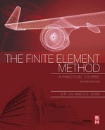
Structures are made of structural components that are in turn made of solids. There are generally four most commonly used structural components: truss, beam, plate, and shell, as shown in Figure 2.1. In physical structures, the main purpose of using these structural components is to effectively utilize the material and reduce the weight and cost of the structure. A practical structure can consist of different types of structural components, including solid blocks. Theoretically, the principles and methodology in solid mechanics can be applied to solve a mechanics problem for all structural components, but this is usually not a very efficient method. Theories and formulations for taking geometrical advantages of the structural components have therefore been developed. Formulations for a truss, a beam, 2D solids, and plate structures will be discussed in this chapter. In engineering practice, plate elements are often used together with two-dimensional solids for modeling shells. Therefore in this book, shell structures will be modeled by combining plate elements and 2D solid elements, without the use of classic theories for (curved) shells.
2.2 Equations for three-dimensional solids
2.2.1 Stress and strain
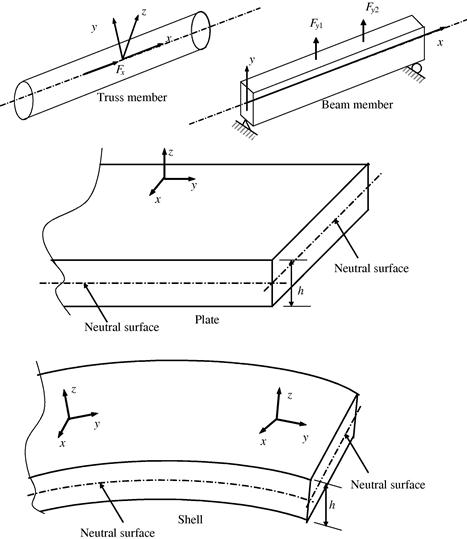
Let’s consider a continuous three-dimensional (3D) elastic solid with a volume V and a surface S, as shown in Figure 2.2. The surface of the solid is further divided into two types: A surface on which the external forces are prescribed is denoted SF; and a surface on which the displacements are prescribed is denoted Sd. The solid can also be loaded by body force fb and surface force fs in any distributed fashion in the volume of the solid.
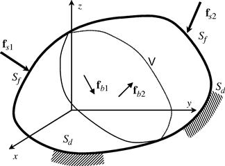
Figure 2.2 Solid subjected to forces applied within the solid (body force) and on the surface of the solid (surface force).
At any point in the solid, the components of stress are indicated on the surface of an “infinitely” small cubic volume, as shown in Figure 2.3. On each surface, there will be the normal stress component, and two components of shearing stress. The sign convention for the subscript is that the first letter represents the surface on which the stress is acting, and the second letter represents the direction of the stress. The directions of the stresses shown in the figure are taken to be the positive directions. By taking moments of forces about the central axes of the cube at the state of equilibrium, it is easy to confirm the shear equivalence relations:
![]() (2.1)
(2.1)
Therefore, there are six independent stress components in total at a point in 3D solids. These stresses are often called stress tensors (because they obey the rules of coordinate transformation for tensors). They can often be written (especially in the FEM) in a vector form of:
![]() (2.2)
(2.2)
Corresponding to the six stress tensors, there are six strain components at any point in a solid, which can also be written in a similar vector form of:
![]() (2.3)
(2.3)
Notice that we use the engineering notation of γij (engineering shear strain) instead of the tensor notation of εij (=γij/2) for shear strain components in the vector form of strains. Strain is essentially the change of displacements per unit length, and therefore the components of strain in a 3D solid can be obtained from the derivatives of the displacements as follows:
 (2.4)
(2.4)
where u, v, and w are the displacement components in the x, y, and z directions, respectively. The six strain–displacement relationships in Eq. (2.4) can be rewritten in the following matrix form:
![]() (2.5)
(2.5)
where U is the displacement vector, and has the form of:
 (2.6)
(2.6)
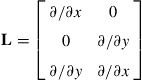
and L is a matrix of partial differential operators obtained simply by inspection of Eq. (2.4):
 (2.7)
(2.7)
2.2.2 Constitutive equations
The constitutive equation gives the relationship between the stress and strain in the material of a solid. It is often termed Hooke’s law. The original Hooke’s law is derived only for a 1D bar. The generalized Hooke’s law for 3D anisotropic materials can be given in the following matrix form:
![]() (2.8)
(2.8)
where c is a matrix of material constants, which are normally obtained through experiments. The constitutive equation can be written explicitly as:
 (2.9)
(2.9)
Note that, since cij = cji, there are altogether 21 independent material constants cij, which is the case for a fully anisotropic material. For isotropic materials, however, c can be reduced to:
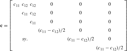 (2.10)
where
![]() (2.11)
(2.11)
in which E, υ, and G are Young’s modulus, Poisson’s ratio, and the shear modulus of the material, respectively. There are only two independent constants among these three constants. The relationship between these three constants is:
![]() (2.12)
(2.12)
That is to say, for any isotropic material, given any two of the three constants, the other one can be calculated using the above equation.
2.2.3 Dynamic equilibrium equations
To formulate the dynamic equilibrium equations, let’s consider an infinitesimal block of solid, shown in Figure 2.4. As in forming all equilibrium equations, equilibrium of forces is required in all directions. Note that, since this is a general, dynamic system, we also have to consider the inertial forces of the block. The equilibrium of forces in the x direction gives:
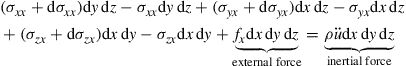 (2.13)
where the term on the right-hand side of the equation is the inertial force term with ρ being the density of the material, and fx is the distributed external body force (density) evaluated at the center of the small block. Note that:
![]() (2.14)
(2.14)
Hence, Eq. (2.13) becomes one of the equilibrium equations, written as:
![]() (2.15)
(2.15)
Similarly, the equilibrium of forces in the y and z directions results in two other equilibrium equations:
![]() (2.16)
(2.16)
![]() (2.17)
(2.17)
This set of three equilibrium equations, Eqs. (2.15) to (2.17), can be written in a concise matrix form:
![]() (2.18)
(2.18)
where fb is the vector of external body forces in the x, y, and z directions:
 (2.19)
Using Eqs. (2.5) and (2.8), the equilibrium equation Eq. (2.18) can be further written in terms of displacements:
![]() (2.20)
(2.20)
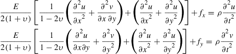
The above is the general form of the dynamic equilibrium equation expressed as a matrix equation. We note that since L is a matrix of first order differential operators [see Eq. (2.7)]; ![]() will be a matrix of second order differential operators. Therefore, Eq. (2.20) is a set of three second order partial differential equations (PDEs), which can be seen more clearly if we expand equation Eq. (2.20) in detail (for isotropic materials):
will be a matrix of second order differential operators. Therefore, Eq. (2.20) is a set of three second order partial differential equations (PDEs), which can be seen more clearly if we expand equation Eq. (2.20) in detail (for isotropic materials):
 (2.20a)
If the loads applied on the solid are static, the only concern is then the static status of the solid. Hence, the static equilibrium equation can be obtained simply by dropping the dynamic term (the inertial force term) in Eq. (2.20):
![]() (2.21)
(2.21)

2.2.4 Boundary conditions
There are two types of boundary conditions: displacement (essential) and force/stress (natural) boundary conditions. The displacement boundary condition can be simply written as:
![]() (2.22)
(2.22)
on displacement boundaries. The bar stands for the prescribed value for the displacement component. For most of the actual simulations, the displacement is used to describe the support or constraints on the solid, and hence the prescribed displacement values are often zero. In such cases, the boundary condition is termed a homogenous boundary condition. Otherwise, they are inhomogenous boundary conditions.
The force boundary conditions are often written as:
![]() (2.23)
(2.23)
on force/stress boundaries, where n is given by:
 (2.24)
in which ni (i = x, y, z) are cosines of the outwards normal on the boundary. The bar stands for the prescribed value for the force component. A force boundary condition can also be both homogenous and inhomogenous. If the condition is homogenous, it implies that the boundary is a free surface.
The displacement boundary condition and the force boundary condition are usually “complementary:” when the displacements are pre-specified on a part of the boundary, the force there is in general not known, and when the force is pre-specified on a part of the boundary, the displacements there are, in general, not known. In other words, we cannot pre-specify both of them at the same location on the boundary, but only one of them. Otherwise, they can be “contradictary,” and the problem may become an ill-posed one. Special measures are required for dealing with such ill-posed problems (see Liu and Han, 2003).
The reader may naturally ask why the displacement boundary condition is called an essential boundary condition and the force boundary condition is called a natural boundary conditions. This is also related to the complementary nature of these two types of boundary conditions. The terms “essential” and “natural” come from the use of the so-called weak form formulation (such as the one used in FEM) for deriving system equations using assumed displacement methods. In such a formulation process, the displacement condition has to be satisfied first before derivation starts, or the process will fail. Therefore, the displacement condition is essential. As long as the essential (displacement) condition is satisfied, the weak formulation process will lead to the equilibrium equations as well as the force boundary conditions. This means that the force boundary condition is naturally derived from the process, and it is therefore called the natural boundary condition. Since the terms essential and natural boundary do not describe the physical meaning of the problem, it is actually a mathematical term, and they are also used for problems other than in mechanics.
With a well defined set of equilibrium equations with a body force, displacement, and force boundary conditions, analytical means can then be applied to solve the problem for displacements and stress, if the setting of the problem is sufficiently simple and problem domain is “regular.” Detailed descriptions can be found in any book on elasticity such as the ones by Fung (1965), and Timoshenko and Goodier (1970). This book aims to solve the equations system through the FEM for problems of general complexity.
Equations obtained in this section are applicable to 3D solids. The objective of most analysts is to solve the equilibrium equations and obtain the solution of the field variable, which in this case is the displacement. Theoretically, these equations can be applied to all other types of structures such as trusses, beams, plates, and shells, because physically they are all 3D in nature. However, treating all the structural components as 3D solids makes computation very expensive, and sometimes practically impossible. Therefore, theories for taking geometrical advantage of different types of solids and structural components have been developed. Application of these theories in a proper manner can reduce the analytical and computational effort drastically. A brief description of these theories is given in the following sections.
2.3 Equations for two-dimensional solids
2.3.1 Stress and strain
Three-dimensional problems can be drastically simplified if they can be treated as a two-dimensional (2D) solid. For representation as a 2D solid, we basically remove one coordinate (usually the z axis), and hence assume that all the dependent variables are independent of the z axis, and all the external loads are also independent of the z coordinate, and applied only in the x–y plane. Therefore, we are left with a system with only two coordinates, x and y.
There are primarily two types of 2D solids. One is a plane stress solid, and the other is a plane strain solid. Plane stress solids are solids whose thickness in the z direction is very small compared with dimensions in the x and y directions. External forces are applied only in the x–y plane, and stresses in the z direction (σzz, σxz, σyz) are all zero, as shown in Figure 2.5. Plane strain solids are those solids whose thickness in the z direction is very large compared with the dimensions in the x and y directions. External forces are applied evenly along the z axis, and the movement in the z direction at any point is constrained. The strain components in the z direction (εzz, γxz, γyz) are, therefore, all zero, as shown in Figure 2.6.
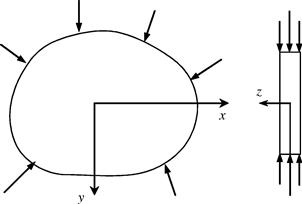
Figure 2.5 Plane stress problem. The dimension of the solid in the thickness (z) direction is much smaller than that in the x and y directions. All the forces are applied within the x–y plane and hence the displacements are functions of x and y only.
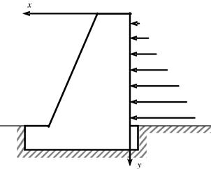
Figure 2.6 Plane strain problem. The dimension of the solid in the thickness (z) direction is much larger than that in the x and y directions, and the cross-section and the external forces do not vary in the z direction. A cross-section can then be taken as a representative cell, and hence the displacements are functions of x and y only.
Note that for the plane stress problems, the strains γxz and γyz are zero, but εzz will not be zero. It can be recovered easily using Eq. (2.9) after the in-plane stresses are obtained. Similarly, for the plane strain problems, the stresses σxz and σyz are zero, but σzz will not be zero. It can be recovered easily using Eq. (2.9) after the in-plane strains are obtained.
The system equations for 2D solids can be obtained immediately by omitting terms related to the z direction in the system equations for 3D solids. The stress components are:
 (2.25)
There are three corresponding strain components at any point in 2D solids, which can also be written in a similar vector form:
 (2.26)
The strain–displacement relationships are:
![]() (2.27)
(2.27)
where u and v are the displacement components in the x and y directions, respectively. The strain–displacement relation can also be written in the following matrix form:
![]() (2.27a)
(2.27a)
where the displacement vector has the form of:
 (2.28)
and the differential operator matrix is obtained simply by inspection of Eq. (2.27) as:
 (2.29)
2.3.2 Constitutive equations
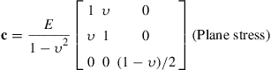
Hooke’s law for 2D solids has the following matrix form with σ and ε from Eqs. (2.25) and (2.26):
![]() (2.30)
(2.30)
where c is a matrix of material constants, which have to be obtained through experiments. For plane stress, isotropic materials, we have:
 (2.31)
To obtain the plane stress c matrix above, the conditions of σzz = σxz = σyz = 0 are imposed on the generalized Hooke’s law for isotropic materials. For plane strain problems, εzz = γxz = γyz = 0 are imposed, or alternatively, replace E and ν in Eq. (2.31), respectively, with E/(1 – υ2) and υ/(1 – υ2), which leads to:
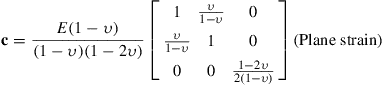 (2.32)
The displacement and force boundary conditions can be written in a similar way as for the 3D solids.
2.3.3 Dynamic equilibrium equations
The dynamic equilibrium equations for 2D solids can be easily obtained by removing the terms related to the z coordinate from the 3D counterparts of Eqs. (2.15)–(2.17):
![]() (2.33)
(2.33)
![]() (2.34)
(2.34)
These equilibrium equations can be written in a concise matrix form of:
![]() (2.35)
(2.35)
where fb is the external force vector given by:
 (2.36)
The expanded equation of Eq. (2.35) for 2D plane stain and isotropic materials becomes:
 (2.36a)
It is clearly seen again that it is a set of second order partial differential equations (PDEs).
For static problems, the dynamic inertia term is removed, and the equilibrium equations can be written as:
![]() (2.37)
(2.37)
Equations (2.35) or (2.37) will be much easier to solve and computationally less expensive as compared with equations for the 3D solids.
2.4 Equations for truss members
A typical truss structure is shown in Figure 2.7. Each truss member in a truss structure is a solid whose dimension in one direction is much larger than in the other two directions, as shown in Figure 2.8. The force is applied only in the direction with larger dimension, usually the x direction. Therefore a truss member is actually a one-dimensional (1D) solid. The equations for 1D solids can be obtained by further omitting the stress related to the y direction, σyy, σxy, from the 2D case.

Figure 2.7 A typical structure made up of truss members. The entrance of the faculty of Engineering, National University of Singapore.

Figure 2.8 Truss member. The cross-sectional dimension of the solid is much smaller than that in the axial (x) directions, and the external forces are applied in the x direction, hence the axial displacement is a function of x only.
2.4.1 Stress and strain
Omitting the stress terms in the y direction, the stress in a truss member is only σxx, which is often simplified as σx. The corresponding strain in a truss member is εxx, which is simplified as εx. The strain–displacement relationship is simply given by:
![]() (2.38)
(2.38)
2.4.2 Constitutive equations
Hooke’s law for 1D solids has the following simple form, with the exclusion of the y dimension and hence the Poisson effect:
![]() (2.39)
(2.39)
This is actually the original Hooke’s law. The Young’s module E can be obtained using a simple tensile test.
2.4.3 Dynamic equilibrium equations
By eliminating the y dimension term from Eq. (2.33), the dynamic equilibrium equation for 1D solids is:
![]() (2.40)
(2.40)
Substituting Eqs. (2.38) and (2.39) into Eq. (2.40), we obtain the governing equation for elastic and homogenous (E is independent of x) trusses as follows:
![]() (2.41)
(2.41)
The static equilibrium equation for trusses is obtained by eliminating the inertia term in Eq. (2.40):
![]() (2.42)
(2.42)
The static equilibrium equation in terms of displacement for elastic and homogenous trusses is obtained by eliminating the inertia term in Eq. (2.41):
![]() (2.43)
(2.43)
For bars of constant cross-sectional area A, the above equation can be written as:
![]() (2.43a)
(2.43a)
where Fx = fxA is the external force applied in the axial direction of the bar, in which A is the cross-sectional area of the bar.
Solution
We can derive the solution via analytical methods, as this problem is very simple. From the strong form of the governing equation, Eq. (2.43), we have:
![]()
This is because the bar is free of body forces, or fx = 0. The general solution that satisfies the previous governing equation can be obtained very easily as:
![]()
where c0 and c1 are unknown constants to be determined by boundary conditions. We need now to find the particular solution that satisfies the boundary condition of the physical (mechanics) problem. The displacement boundary condition for this problem can be given as:
![]()
Therefore, we have c0 = 0. The displacement now becomes:
![]()
Using Eqs. (2.38) and (2.39), we obtain:
![]()
The force boundary condition at x = l for this bar can be given as:
![]()
Equating the right-hand side of the previous two equations, we obtain:
![]()
The stress at any point in the bar is obtained by:
![]()
which is uniform throughout the bar. We finally obtain the particular solution of the displacement of the bar:
![]()
At x = l, we have the maximum displacement.
![]()
Although this problem is very simple, it shows a typical approach to solving a differential equation analytically for exact solutions:
• Obtain the general solution that satisfies the governing equations containing unknown constants.
• Use the boundary conditions for the problem to determine these constants, leading to a particular solution that satisfies both the governing equation and the boundary conditions.
2.5 Equations for beams
A beam possesses geometrically similar dimensional characteristics to a truss member, as shown in Figure 2.9. The difference is that the forces applied on beams are transversal, meaning the direction of the force is perpendicular to the axis of the beam. Therefore, a beam experiences bending, which is the deflection in the y direction as a function of x.

Figure 2.9 Simply supported beam. The cross-sectional dimensions of the solid are much smaller than those in the axial (x) directions, and the external forces are applied in the transverse (y) direction, hence the deflection of the beam is a function of x only.
2.5.1 Stress and strain
The stresses on the cross-section of a beam are the normal stress, σxx, and shear stress, σxz. There are several theories for analyzing beam deflections. These theories can be basically divided into two major categories: a theory for thin beams and a theory for thick beams. This book focuses on the thin beam theory, which is often referred to as the Euler–Bernoulli beam theory. The Euler–Bernoulli beam theory assumes that the plane cross-sections, which are normal to the undeformed centroidal axis, remain plane after bending and remain normal to the deformed axis, as shown in Figure 2.10. With this assumption, one can first have:
![]() (2.44)
(2.44)
which simply means that the shear stress is assumed to be negligible. Secondly, assume that the centroidal axis of the beam is not stretched or compressed in the x direction. Using the 3rd equation in Eq. (2.27), the axial displacement, u, of a fiber at a distance y from the centroidal axis can be expressed by:
![]() (2.45)
(2.45)
where θ is the rotation of the cross-section of the beam in the x–y plane measured counterclockwise. The rotation can be obtained from the deflection of the centroidal axis of the beam, v, in the y direction:
![]() (2.46)
(2.46)
The relationship between the normal strain and the deflection can be given by:
![]() (2.47)
(2.47)
where L is the differential operator, given by:
![]() (2.48)
(2.48)

2.5.2 Constitutive equations
Similar to the equation for truss members, the original Hooke’s law is applicable for beams:
![]() (2.49)
(2.49)
2.5.3 Moments and shear forces
Because the loading on the beam is in the transverse direction, there will be moments and corresponding shear forces resulted in the cross-sectional plane of the beam. In addition, bending of the beam can also be achieved if pure moments are applied instead of transverse loading. Figure 2.11 shows a small representative cell of length dx of the beam. The beam cell is subjected to external force, Fy = Afy, moment, M, shear force, Q, and inertial force, ![]() , where ρ is the density of the material and A is the area of the cross-section. The moment on the cross-section at x results from the distributed normal stress σxx, as shown in Figure 2.12. The normal stress can be calculated by substituting Eq. (2.47) into Eq. (2.49):
, where ρ is the density of the material and A is the area of the cross-section. The moment on the cross-section at x results from the distributed normal stress σxx, as shown in Figure 2.12. The normal stress can be calculated by substituting Eq. (2.47) into Eq. (2.49):
![]() (2.50)
(2.50)
It can be seen from the above equation that the normal stress σxx varies linearly with respect to y in the vertical direction on the cross-section of the beam. The moments resulting from the normal stress on the cross-section can be calculated by the following integration over the area of the cross-section:
![]() (2.51)
(2.51)
where I is the second moment of area (or moment of inertia) of the cross-section with respect to the z axis, which can be calculated for a given shape of the cross-section using the following equation:
![]() (2.52)
(2.52)
Using Eqs. (2.50–2.52), we shall have:
![]()
We now consider the force equilibrium of the small beam cell in the z direction:
![]() (2.53)
(2.53)
or
![]() (2.54)
(2.54)
We would also need to consider the moment equilibrium of the small beam cell with respect to any point at the right surface of the cell:
![]() (2.55)
(2.55)
Neglecting the small second order term containing (dx)2 leads to:
![]() (2.56)
(2.56)
Finally, substituting Eq. (2.51) into Eq. (2.56) gives:
![]() (2.57)
(2.57)
Equations (2.56) and (2.57) give the relationships between the moments, shear forces, and the deflection of the Euler–Bernoulli beam.


2.5.4 Dynamic equilibrium equations
The dynamic equilibrium equation for beams can be obtained simply by substituting Eq. (2.57) into Eq. (2.54):
![]() (2.58)
(2.58)
The static equilibrium equation for beams can be obtained similarly by dropping the dynamic term in Eq. (2.58):
![]() (2.59)
(2.59)
The displacement boundary conditions for beams will be given in terms of deflection v and rotation θ, respectively, which are complementary to the force boundary conditions in terms of shear force Q and moments M (see Timoshenko and Gere, 1972).
2.6 Equations for plates
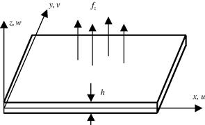
The wings of an aircraft can sometimes be simplified as a plate structure carrying transverse loads in the form of the weight of the engines or other components, as shown in Figure 2.13. A plate possesses a geometrically similar dimensional characteristic to that of a 2D solid, as shown in Figure 2.14. The difference is that the direction of the forces applied on a plate are perpendicular to the plane of the plate. A plate can also be viewed as a 2D analogy of a beam. Therefore, a plate experiencing bending results in deflection w in the z direction, which is a function of x and y.

2.6.1 Stress and strain
The stress σzz in a plate is assumed to be zero. Similar to beams, there are several theories for analyzing deflection in plates. These theories can also be basically divided into two major categories: theory for thin plates and theory for thick plates. This chapter addresses a thin plate theory, often called the Classical Plate Theory (CPT), or the Kirchhoff plate theory, as well as the first order shear deformation theory for thick plates known as the Reissner–Mindlin plate theory (Reissner, 1945; Mindlin, 1951). Note that pure plate elements are usually not available in most commercial finite element packages, since most people would use the more general shell elements, which will be discussed in later chapters. Notice also that the formulation for elements for CPT plates is quite similar to that for beams (with just an extension for one more dimension). Hence, in this book, only finite element equations of plate elements based on the Reissner–Mindlin plate theory will be formulated (Chapter 8). Nevertheless, the CPT will also be briefed in this chapter for completeness of this introduction to mechanics for solids and structures.
The CPT assumes that normals to the middle (neutral) plane of the undeformed plate remain straight and orthogonal to the middle plane during deformation or bending. This assumption results in:
![]() (2.60)
(2.60)
Secondly, assume that the middle plan of the plate is not stretched or compressed in the x-y plane. Using the last two equations in Eq. (2.4), the displacements parallel to the—middle plane, u and v, at a distance z from the middle plane, can be expressed by:
![]() (2.61)
(2.61)
![]() (2.62)
(2.62)
where w is the deflection of the middle plane of the plate in the z direction. The relationship between the components of strain and the deflection can be given by:
![]() (2.63)
(2.63)
 (2.64)
![]() (2.65)
(2.65)
![]() (2.66)
(2.66)
where ε is the vector of in-plane strains defined by Eq. (2.26), and L is the differential operator matrix given, in this case, by:
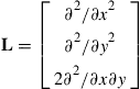 (2.67)
2.6.2 Constitutive equations
The original Hooke’s law is applicable for plates:
![]() (2.68)
(2.68)
where c has the same form for 2D solids defined by Eq. (2.31) for the plane stress case, since σzz is assumed to be zero.
2.6.3 Moments and shear forces
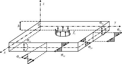
Figure 2.15 shows a small representative cell of dx × dy from a plate of thickness h. The plate cell is subjected to external force fz (force per unit area) and inertial force ![]() , where ρ is the density of the material. Figure 2.16 shows the moments Mx, My, Mz, and Mxy, and shear forces Qx and Qy present. The moments and shear forces result from the distributed normal and shear stresses σxx, σyy, and σxy, shown in Figure 2.15. The stresses can be obtained by substituting Eq. (2.66) into Eq. (2.68):
, where ρ is the density of the material. Figure 2.16 shows the moments Mx, My, Mz, and Mxy, and shear forces Qx and Qy present. The moments and shear forces result from the distributed normal and shear stresses σxx, σyy, and σxy, shown in Figure 2.15. The stresses can be obtained by substituting Eq. (2.66) into Eq. (2.68):
![]() (2.69)
(2.69)
It can be seen from the above equation that the normal stresses vary linearly with respect to z in the thickness direction of the plate. The moments on the cross-section can be calculated in a similar way as for beams via the following integration:
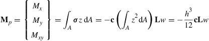 (2.70)
Consider first the equilibrium of the small plate cell in the z direction, and note that dQx = (∂Qx/∂x)dx and dQy = (∂Qy/∂y)dy, we have:
![]() (2.71)
(2.71)
or
![]() (2.72)
(2.72)
Consider then the moment equilibrium of the plate cell with respect to the y axis, and neglecting the small second order term, this leads to a formula for shear force Qx:
![]() (2.73)
(2.73)
Finally, consider the moment equilibrium of the plate cell with respect to the x axis, and neglecting the small second order term, this gives:
![]() (2.74)
(2.74)
in which we implied that Myx = Mxy.

2.6.4 Dynamic equilibrium equations
To obtain the dynamic equilibrium equation for plates, we first substitute Eq. (2.70) into Eqs. (2.73) and (2.74), after which Qx and Qy are substituted into Eq. (2.72):
 (2.75)
where D = Eh3/(12(1 − υ2)) is the bending stiffness of the plate. The static equilibrium equation for plates can again be obtained by dropping the dynamic term in Eq. (2.75):
 (2.76)
Similarly to the beam case, the displacement boundary conditions for beams will be given in terms of deflection v and rotation θ, respectively, complementary to the force boundary conditions in terms of shear force Q and moments M (see Timoshenko, 1940).
2.6.5 Reissner–Mindlin plate
The Reissner–Mindlin plate theory (Reissner, 1945; Mindlin, 1951) is applied for thick plates, where the shear deformation and rotary inertia effects are included. The Reissner–Mindlin theory does not require the cross-section to be perpendicular to the axial axes after deformation, as shown in Figure 2.17. Therefore, γxz ≠ 0 and γyz ≠ 0. The displacements parallel to the undeformed middle surface, u and v, at a distance z from the middle plane can be expressed as:
![]() (2.77)
(2.77)
![]() (2.78)
(2.78)
where θx and θy are, respectively, the rotations about the x and y axes of lines normal to the middle plane before deformation.

Figure 2.17 Shear deformation in a Mindlin plate. The rotations of the cross-sections are treated as independent variables.
The in-plane strains defined by Eq. (2.26) are given by:
![]() (2.79)
(2.79)
where L, in this case, is given by:
 (2.80)
and
 (2.81)
Using Eq. (2.4), the transverse shear strains γxz and γyz can be obtained as:
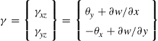 (2.82)
Note that if the transverse shear strains are negligible, the above equation will lead to:
![]() (2.83)
(2.83)
![]() (2.84)
(2.84)
and Eq. (2.79) becomes Eq. (2.66) of the CPT. The transverse average shear stress τ relates to the transverse shear strain in the form:
 (2.85)
where G is the shear modulus, and κ is a constant of shear correction factor to account for the assumption that the shear strain is constant across the thickness of the plate. κ is usually taken to be π2/12 or 5/6.
The equilibrium equations for a Reissner–Mindlin plate can also be similarly obtained as that of a thin plate. Equilibrium of forces and moments can be carried out but this time taking into account the transverse shear stress and rotary inertia. For the purpose of this book, the above concepts for the Reissner–Mindlin plate will be sufficient and the equilibrium equations will not be shown here. Chapter 8 will detail the derivation of the discrete finite element equations by using energy principles.
2.7 Remarks
Having shown how the equilibrium equations for various types of geometrical structures are obtained, it is noted that all the equilibrium equations are just special cases of the general equilibrium equation for 3D solids. The use of proper assumptions and theories can lead to a dimension reduction, and hence simplify the problem. These kinds of simplification can significantly reduce the size of finite element models.
2.8 Review questions
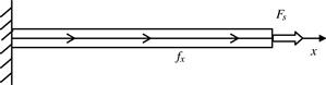
1. Consider the problem of a 1D bar of uniform cross-section, as shown in Figure 2.18. The bar is fixed at the left end and is of length l = 1 m and section area A = 0.0001 m2. It is subjected to a uniform body force fx and a concentrated force Fs at the right end. The Young’s modulus of the material is ![]() . Using the analytical (exact) method, obtain solutions in terms of the distribution and the maximum value of the displacement, strain, and stress, for the following cases:
. Using the analytical (exact) method, obtain solutions in terms of the distribution and the maximum value of the displacement, strain, and stress, for the following cases:
b. fx = 1000 N/m and Fs = 1000 N.
c. fx = (100x + 1000) N/m and Fs = 0.
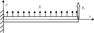
2. Consider a cantilever beam of uniform cross-section, as shown in Figure 2.19. The beam is clamped at the left end and is of length l = 1 m and with a square section area of A = 0.001 m2. It is subjected to a uniform body force fb and a concentrated force Fs at the right end. The Young’s modulus of the material is ![]() . Using the analytical (exact) method, obtain solutions in terms of the distribution and the maximum value of the deflection, moment, shear force, and normal stresses, for the following cases:
. Using the analytical (exact) method, obtain solutions in terms of the distribution and the maximum value of the deflection, moment, shear force, and normal stresses, for the following cases:
References
1. Fung YC. Foundations of Solid Mechanics. Englewood Cliffs: Prentice-Hall; 1965.
2. Hu HC. Variational Principles in Elasticity and Applications. Scientific Publication 1982; (in Chinese).
3. Liu GR, Han X. Computational Inverse Techniques in Nondestructive Evaluation. CRC Press 2003.
4. Mindlin RD. Influence of rotary inertia and shear on flexural motion of isotropic elastic plates. Journal of Applied Mechanics. 1951;18:31–38.
5. Reissner E. The effect of transverse shear deformation on the bending of elastic plates. Journal of Applied Mechanics. 1945;67:A67–A77.
6. Timoshenko S. Theory of Plates and Shells. London: McGraw-Hill; 1940.
7. Timoshenko SP, Gere J. Mechanics of Materials. Van Nostrand Reinhold Company 1972.
8. Timoshenko SP, Goodier JN. Theory of Elasticity. third ed. New York: McGraw-Hill; 1970.
9. Xu ZL. Elasticity. vols. 1 and 2 People’s Education Press 1979; (in Chinese).