
Fundamentals for Finite Element Method
3.1 Introduction
As mentioned in Chapter 1, when using the finite element method (FEM) to solve mechanics problems governed by a set of partial differential equations, the problem domain is first discretized (in a proper manner) into a set of small elements. In each of these elements, the variation/profile/pattern of the displacements is assumed in simple forms to obtain element equations. The equations obtained for each element are then assembled together with adjoining elements to form the global finite element equation for the whole problem domain. Equations thus created for the global problem domain can be solved easily for the entire displacement field.
The above-mentioned FEM process does not seem to be a difficult task. However, upon close examination of the process, one would naturally ask a series of questions. How can one simply assume the profile of the solution of the displacement in any simple form? How can one ensure that the governing partial differential equations will be satisfied by the assumed displacement? What should one do when using the assumed profile of the displacement to determine the final displacement field? Yes, one can just simply assume the profile of the solution of the displacements, but a principle has to be followed in order to obtain discretized system equations that can be solved routinely for the final displacement field. The use of such a principle guarantees the best (may not be exact) satisfaction of the governing system equation under certain conditions. The following details one of the most important principles, which will be employed to establish the FEM equations for mechanics problems of solids and structures.
Perhaps, for a beginner, full understanding of the details of the equations in this chapter may prove to be a challenging task. It is thus advised that the novice reader just understands the basic concepts involved without digging too much into the equations. It is then recommended to review this chapter again, after going through subsequent chapters, with examples to fully understand the equations. Advanced readers are referred to the FEM handbook (Kardestuncer, 1987) for more complete topics related to FEM.
3.2 Strong and weak forms: problem formulation
The partial differential system equations developed in Chapter 2, such as Eqs. (2.20) and (2.21) with boundary conditions, Eqs. (2.22) and (2.23), are strong forms of the governing system of equations for solid mechanics problems. The strong form, in contrast to a weak form, requires strong continuity on the dependent field variables (the displacements u, v, and w in this case). By “strong,” we mean that the functions used to approximate the field variables have to be differentiable up to the order of the partial differential equations (the strong form of the system equations). Obtaining the exact solution for a strong form of the system equation is usually very difficult for practical engineering problems. The finite difference method (FDM) can be used to solve system equations of the strong form to obtain an approximated solution. However, the method usually works well only for problems with simple and regular geometry and boundary conditions.
A weak form of the system equations is usually created using one of the following widely used methods:
• Energy principles (see, for example, Washizu, 1974; Reddy, 1984; Liu, 2009).
• Weighted residual methods (see, for example, Crandall, 1956; Finlayson and Scriven, 1966; Finlayson, 1972; Zienkiewicz and Taylor, 2000; Liu, 2009; Liu and Zhang, 2013).
The energy principle can be categorized as a special form of the variational principle which is particularly suited to problems of the mechanics of solids and structures. The weighted residual method is a more general mathematical tool applicable, in principle, for solving all kinds of partial differential equations. Both methods are very easy to understand and apply. This book will demonstrate both methods for creating FEM equations. An energy principle will be used for mechanics problems of solids and structures, and the weighted residual method will be used for formulating the heat transfer problems. It is also equally applicable to use the energy principle for heat transfer problems, and the weighted residual method for solid mechanics problems, and the procedure is very much the same. A comprehensive discussion on the differences and terminologies on energy methods, variation methods, functional analysis approaches, weak form methods, and weakened weak form methods can be found in the mesh-free book by Liu (2009), and the recent book on the smoothed point interpolation method (S-PIM) by Liu and Zhang (2013).
The weak form is often an integral form and requires a weaker continuity on the field variables. Due to the weaker requirement on the field variables, and the integral operation, a formulation based on a weak form usually produces a set of discretized system equations that give much more stable (and hence reliable) and accurate results, especially for problems of complex geometry. Hence, the weak form is preferred by many for obtaining an approximate solution. The FEM is a typical example of successfully using weak form formulations. Using the weak form usually leads to a set of well-behaved algebraic system equations, if the problem domain is discretized properly into elements. As the problem domain can be discretized into different types of elements, the FEM can be applied for many practical engineering problems with most kinds of complex geometry and boundary conditions.
In the following section, Hamilton’s principle, which is one of the most powerful energy principles, is introduced for FEM formulation of problems of mechanics of solids and structures. Hamilton’s principle is chosen because it is simple and can be used for dynamic problems. The approach adopted in this book is to directly work out the dynamic system equations, after which the static system equations can be easily obtained by simply dropping out the dynamic terms. This can be done because of the simple fact that the dynamic system equations are the general system equations, and the static case can be considered to be just a special case of the dynamic equations.
3.3 Hamilton’s principle: A weak formulation
3.3.1 Hamilton’s principle
Hamilton’s principle is a simple yet powerful tool that can be used to derive discretized dynamic system equations. It states simply that,
Of all the admissible time histories of displacement the most accurate solution makes the Lagrangian functional stationary.
An admissible displacement must satisfy the following conditions:
Condition (a) ensures that the displacements are compatible (continuous) in the problem domain. As will be seen in Chapter 11, there are situations when incompatibility can occur at the edges between elements. Condition (b) ensures that the displacement constraints are satisfied; and condition (c) requires the displacement history to satisfy the constraints at the initial and final times.
Mathematically, Hamilton’s principle states:
![]() (3.1)
(3.1)
The Langrangian functional, L, is obtained using a set of admissible time histories of displacements, and it consists of
![]() (3.2)
(3.2)
where T is the kinetic energy, Π is the potential energy (for our purposes, it is the elastic strain energy), and Wf is the work done by the external forces. It is clear that the Langrangian functional L is some kind of potential energy of the entire system, and thus the kinetic energy and the work done by the external forces results in deduction in paternal energy.
The kinetic energy of the entire problem domain is defined in the integral form
![]() (3.3)
(3.3)
where V represents the whole volume of the solid, and U is the set of admissible time histories of displacements.
The strain energy in the entire domain of elastic solids and structures can be expressed as
![]() (3.4)
(3.4)
where ε are the strains obtained using the set of admissible time histories of displacements. The work done by the external forces over the set of admissible time histories of displacements can be obtained by
![]() (3.5)
(3.5)
where Sf represents the surface of the solid on which the surface forces are prescribed (see Figure 2.2).
Hamilton’s principle allows one to simply assume any set of displacements, as long as it satisfies the three admissible conditions. The assumed set of displacements will not usually satisfy the strong form of governing system equations unless we are extremely lucky, or the problem is extremely simple and we know the exact solution (in this case we do not need to solve the problem). Application of Hamilton’s principle will conveniently guarantee a combination of this assumed set of displacements to produce the most accurate (in the energy norm measure) solution for the system that is governed by the strong form of the system equations.
The power of Hamilton’s principle (or any other variational principle) is that it provides freedom of choice, opportunity, and possibility. For practical engineering problems, one usually does not have to pursue the exact solution, which in most cases is usually unobtainable, because we now have a choice of quite conveniently obtaining a good approximation using Hamilton’s principle, by assuming the likely form, pattern or shape of the solutions. Hamilton’s principle thus provides the foundation for the FEMs. Furthermore, the simplicity of Hamilton’s principle (or any other energy principle) manifests itself in the use of scalar energy quantities. Engineers and scientists like working with scalar quantities when it comes to numerical calculations, as they do not need to worry about the direction. All the mathematical tools required to derive final discrete system equations are basic operations of integration, differentiation, and variation, all of which are standard linear operations. Another plus point of Hamilton’s principle is that the final discrete system equations produced are usually a set of linear algebraic equations that can be solved using conventional methods and standard computational routines. The following demonstrates how the finite element equations can be established using Hamilton’s principle and its simple operations.
3.3.2 Minimum total potential energy principle
For static problems, Hamilton’s principle reduces to the well-known minimum total potential energy principle, which may be stated as,
Of all the admissible displacements the most accurate solution makes the total potential energy minimum.
An admissible displacement must satisfy the following conditions:
Mathematically, the “most” accurate solution is found using
![]() (3.1a)
(3.1a)
The total potential energy, Πt, is obtained using the assume admissible displacement, and it consists of
![]() (3.2a)
(3.2a)
It can be proven for stable materials of a well-posed solid mechanics problem that the stationary point given in (3.1a) is a minimum point of the total potential energy for the solid (see, e.g., Liu, 2009).
3.4 FEM procedure
The standard FEM procedure can be briefly summarized in the following sections.
3.4.1 Domain discretization
The solid or structure is divided into Ne elements with a set of Nn nodes. The procedure is often called meshing, which is usually performed using so-called pre-processors. This is especially true for complex geometries. Figure 3.1 shows an example of a mesh for a two-dimensional solid.

The pre-processor generates unique numbers for all the elements and nodes for the solid or structure in a proper manner. An element is formed by connecting its nodes in a pre-defined consistent fashion to create the connectivity of the element. All the elements together form the entire domain of the problem without any gap or overlapping. It is possible to have different types of elements with different numbers of nodes, as long as they are compatible (no gaps and overlapping; the admissible condition (a) required by Hamilton’s principle) on the boundaries between different elements. In fact, meshes of mixed triangular and quadrilateral elements are frequently used to overcome the difficulties of creating preferable pure quadrilateral elements. The density of the mesh depends upon the accuracy requirement of the analysis and the computational resources available. Generally, a finer mesh will yield results that are more accurate, but will increase the computational cost. As such, the mesh is usually not uniform, with a finer mesh being used in the areas where the displacement gradient is larger or where the accuracy is critical to the analysis. The purpose of the domain discretization is to make it easier in assuming the pattern of the displacement field.
3.4.2 Displacement interpolation
The FEM formulation has to be based on a coordinate system. In formulating FEM equations for elements, it is often convenient to use a local coordinate system that is defined for an element in reference to the global coordination system that is usually defined for the entire structure, as shown in Figure 3.4. Based on the local coordinate system attached on an element, the displacement within the element is now assumed simply by polynomial interpolation using the displacements at its nodes (or nodal displacements) as
 (3.6)
(3.6)
where the superscript h stands for approximation, nd is the number of nodes forming the element, and di is the nodal displacement at the ith node, which is the unknown the analyst wants to find out, and can be expressed in a general form of
 (3.7)
(3.7)
where nf is the number of Degrees Of Freedom (DOF) at a node. For 3D solids, nf = 3, and
 (3.8)
(3.8)
Note that the displacement components can also consist of rotations for structures of beams and plates. The vector de in Eq. (3.6) is the displacement vector for the entire element, and has the form of
 (3.9)
(3.9)
Therefore, the total DOF for the entire element is nd × nf.
In Eq. (3.6), N is a matrix of shape functions for the nodes in the element, which are pre-defined to assume the shapes of the displacement variations with respect to the coordinates. It has the general form of
 (3.10)
where Ni is a sub-matrix of shape functions for displacement components, which is arranged as
 (3.11)
where Nik is the shape function for the kth displacement component, DOF at the ith node. For 3D solids, nf = 3, and often we use Ni1 = Ni2 = Ni3 = Ni. Note that it is not always necessary to use the same shape function for all the displacement components at a node. For example, we often use different shape functions for translational and rotational displacements.
Note that this approach of assuming the displacements is often called the displacement method. Most of the commercially available FEM packages use this approach. There are, however, FEM approaches that assume the stresses instead, but they will not be covered in this book.
3.4.3 Standard procedure for constructing shape functions
Consider an element with nd nodes at xi; (i = 1, 2, …, nd), where xT = {x} for one-dimensional problems, xT = {x y} for two-dimensional problems, and xT = {x y z} for three-dimensional problems. We should have nd shape functions for each displacement component for an element. In the following, we consider only one displacement component in the explanation of the standard procedure for constructing the shape functions. The standard procedure is applicable for any other displacement components. First, the displacement component is approximated in the form of a linear combination of nd linearly-independent basis functions pi(x), i.e.
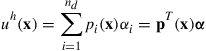 (3.12)
where uh is the approximation of the displacement component, pi(x) is the basis function of monomials in the space coordinates x, and αi is the coefficient for the monomial pi(x). Vector α is defined as
![]() (3.13)
(3.13)
The pi(x) in Eq. (3.12) is built with nd terms of one-dimensional monomials; based on the Pascal’s triangle shown in Figure 3.2 for two-dimensional problems; or the well-known Pascal’s pyramid shown in Figure 3.3 for three-dimensional problems. A basis of complete order of p in the one-dimensional domain has the form
![]() (3.14)
(3.14)
A basis of complete order of p in the two-dimensional domain is provided by
![]() (3.15)
(3.15)
and that in the three-dimensional domain can be written as
 (3.16)
As a general rule, the nd terms of pi(x) used in the basis should be selected from the constant term to higher orders symmetrically from the Pascal triangle shown in Figure 3.2 or Figure 3.3. Some higher order terms can be selectively included in the polynomial basis if there is a need in specific circumstances.


The coefficients αi in Eq. (3.12) can be determined by enforcing the displacements calculated using Eq. (3.12) to be equal to the nodal displacements at the nd nodes of the element. At node i we can have
![]() (3.17)
(3.17)
where di is the nodal value of uh at x = xi. Equation (3.17) can be written in the following matrix form:
![]() (3.18)
(3.18)
where de is the vector that includes the values of the displacement component at all the nd nodes in the element:
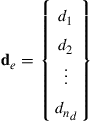 (3.19)
and P is given by
 (3.20)
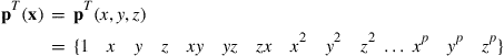
which is called the moment matrix. The expanded form of P is
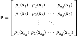 (3.21)
For two-dimensional polynomial basis functions, we may have
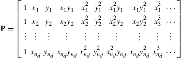 (3.22)
Using Eq. (3.18), and assuming that the inverse of the moment matrix P exists, we can then have
![]() (3.23)
(3.23)
Substituting Eq. (3.23) into Eq. (3.12), we then obtain
 (3.24)
or in matrix form
![]() (3.25)
(3.25)
where N(x) is a matrix of shape functions Ni (x) defined by
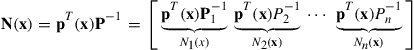 (3.26)
![]()
where ![]() is the ith column of matrix
is the ith column of matrix ![]() , and
, and
![]() (3.27)
(3.27)
The derivatives of the shape functions can be obtained very easily, as all the functions involved are polynomials. The lth derivative of the shape functions is simply given by
![]() (3.28)
(3.28)
3.4.3.1 On the inverse of the moment matrix
In obtaining Eq. (3.23), we have assumed the existence of the inverse of P. There could be cases where P−1 does not exist, and the construction of shape functions will fail. The existence of P−1 depends upon (1) the basis function used, and (2) the nodal distribution of the element. The basis functions have to be chosen first from a linearly-independent set of bases, and then the inclusion of the basis terms should be based on the nodal distribution in the element. The discussion in this direction is more involved, and interested readers are referred to a monograph on mesh-free methods by Liu (2009). In this book, we shall only discuss elements whose corresponding moment matrices are invertible.
3.4.3.2 On the compatibility of the shape functions
The other possible failure of the general procedure of shape function construction is the compatibility of the shape functions created. This is often the case for higher order elements created on physical coordinates. This is the main reason why most of the higher order elements are created in the so-called natural coordinate system (see topics on isoparametric elements). The issues related to the compatibility of element shape functions will be addressed in greater detail in Chapter 11. Note that the compatibility conditions can be relaxed if the S-PIM (Liu and Zhang, 2013) is used. This is because the S-PIM is based on the so-called weakened weak form, and the stability and convergence are ensured by the G-space theory.
3.4.3.3 On other means of construct shape functions
There are many other methods for creating shape functions which do not necessarily follow the standard procedure described above. Some of these often used shortcut methods will be discussed in later chapters, when we develop different types of elements. These shortcut methods need to make use of the properties of shape functions detailed in the next section.
3.4.4 Properties of the shape functions
Property 1
Reproduction property and consistency
The consistency of the shape function within the element depends upon the complete orders of the monomial pi (x) used in Eq. (3.12), and hence is also dependent upon the number of nodes of the element. If the complete order of monomial is k, the shape function is said to possess Ck consistency. To demonstrate, we consider a field given by
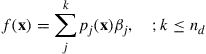 (3.29)
where pj (x) are monomials that are included in Eq. (3.12). Such a given field can always be written using Eq. (3.12) using all the basis terms, including those in Eq. (3.29):
 (3.30)
where
![]() (3.31)
(3.31)
Using n nodes in the support domain of x, we can obtain the vector of nodal function value de as:
 (3.32)
![]()
Substituting Eq. (3.32) into Eq. (3.25), we have the approximation of
 (3.33)
which is exactly what is given in Eq. (3.30). This proves that any field given by Eq. (3.29) will be exactly reproduced in the element by the approximation using the shape functions, as long as the given field function is included in the basis functions used for constructing the shape functions. This feature of the shape function is in fact also very easy to understand by intuition: Any function given in the form of ![]() can be produced exactly by letting αj = βj (j = 1, 2, …, k) and αj = 0 (j = k+1, …, nd). This can always be done as long as the moment matrix P is invertible so as to ensure the uniqueness of the solution for α.
can be produced exactly by letting αj = βj (j = 1, 2, …, k) and αj = 0 (j = k+1, …, nd). This can always be done as long as the moment matrix P is invertible so as to ensure the uniqueness of the solution for α.
The proof of the consistency of the shape function implies another important feature of the shape function: That is the reproduction property, which states that any function that appears in the basis can be reproduced exactly. This important property can be used for creating fields of special features. To ensure that the shape functions have linear consistency, all one needs to do is include the constant (unit) and linear monomials into the basis. We can make use of the feature of the shape function to compute accurate results for problems by including terms in the basis functions that are good approximations of the problem solution. The difference between consistency and reproduction is:
Property 3
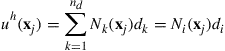
Delta function properties
 (3.34)
where δij is the delta function. The delta function property implies that the shape function Ni of an element should be unit at its home node i, and vanishes at the remote nodes j = i of the element.
The delta function property can be proven easily as follows: because the shape functions Ni(x) are linearly-independent, any vector of length nd should be uniquely produced by linear combination of these nd shape functions. Assume that the displacement at node i is di ≠ 0 and the displacements at other nodes are zero, i.e.
![]() (3.35)
(3.35)
This vector must be uniquely produced by linear combination of these nd shape functions. Substituting the above equation into Eq. (3.24), we have at x = xj, that
 (3.36)
and when i = j, we must have
![]() (3.37)
(3.37)
which (since di ≠ 0) implies that
![]() (3.38)
(3.38)
This proves the first row of Eq. (3.34). When i ≠ j, we must have
![]() (3.39)
(3.39)
which (since again di ≠ 0) requires
![]() (3.40)
(3.40)
This proves the second row of Eq. (3.34). We can then conclude that the shape functions possess the delta function property, as depicted by Eq. (3.34). Note that there are elements, such as the thin beam and plate elements, whose shape functions may not possess the delta function property (see Section 5.2.1 for details).
Property 4
Partitions of unity property
Shape functions are partitions of unity:
 (3.41)
if the constant is included in the basis. This can be proven easily from the reproduction feature of the shape function. Let u(x) = c, where c is an arbitrary non-zero constant; we should have
 (3.42)
which implies the same constant displacement for all the nodes. Substituting the above equation into Eq. (3.24), we obtain
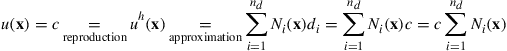 (3.43)
which gives Eq. (3.41). This shows that the partitions of unity of the shape functions in the element allow a constant field or rigid body movement to be reproduced. Note that Eq. (3.41) does not require 0 ≤ Ni (x) ≤ 1.
Property 5
Linear field reproduction
If the first order monomial is included in the basis, the shape functions constructed reproduce the linear field, i.e.
 (3.44)
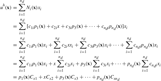
where xi is the coordinate at node i (and similarly for y and z). This can be proven easily from the reproduction feature of the shape function in exactly the same manner for proving Property 4. Let u(x) = x, we should have
![]() (3.45)
(3.45)
Substituting the above equation into Eq. (3.24), we obtain
 (3.46)
which is Eq. (3.44).
Lemma 1
Condition for shape functions being partitions of unity
For a set of shape functions in the general form
![]() (3.47)
(3.47)
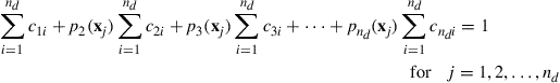
where pi(x) (p1(x) = 1, i = 2, nd) is a set of independent base functions, the sufficient and necessary condition for this set of shape functions being partitions of unity is
![]() (3.48)
(3.48)
where
 (3.49)
Proof
Using Eq. (3.47), the summation of the shape functions is
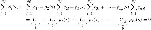 (3.50)
which proves the sufficient condition. To prove the necessary condition, we argue that, to have the partitions of unity, we have
 (3.51)
or
![]() (3.52)
(3.52)
Because pi(x) (p1(x) = 1, i = 2, nd) is a set of independent base functions, the necessary condition for Eq. (3.52) to be satisfied is Eq. (3.48). ![]()
Proof
From Eq. (3.26), we can see that all the nd shape functions are formed via a combination of the same basis function pi(x) (i = 1, 2, …, nd). This feature, together with the delta function property, can ensure the property of partitions of unity. To prove this, we write a set of shape functions in the general form
![]() (3.53)
(3.53)
where we ensured the inclusion of the constant basis of p1(x) = 1. The other basis function pi(x) (i = 2, …, nd) in Eq. (3.53) can be monomials or any other type of basis functions as long as all the basis functions (including p1(x)) are linearly-independent.
From the Condition 2, the shape functions possess a delta function property that leads to
 (3.54)
Substituting Eq. (3.53) into the previous equations, we have
 (3.55)
or
![]() (3.56)
(3.56)
Expanding Eq. (3.56) gives
 (3.57)
or in the matrix form
 (3.58)
Note that the coefficient matrix of Eq. (3.58) is the moment matrix that has a full rank (Condition 1); we then have
![]() (3.59)
(3.59)
The use of Lemma 1 proves the partitions of the unity property of shape functions. ![]()
To prove this, we write a set of shape functions in the following general form of
![]() (3.60)
(3.60)
where we ensure inclusion of the complete linear basis functions of p2(x) = x. The other basis function pi(x) (i = 1, 3, …, nd) in Eq. (3.53) can be monomials or any other type of basis function as long as all the basis functions are linearly-independent.
Consider a linear field of u(x) = x, we should have the nodal vector as follows:
![]() (3.61)
(3.61)
Substituting the above equation into Eq. (3.24), we obtain
 (3.62)
At the nd nodes of the element, we have nd equations:
 (3.63)
Using the delta function property of the shape functions, we have
 (3.64)
Hence, Eq. (3.63) becomes
 (3.65)
Or in matrix form,
 (3.66)
Note that the coefficient matrix of Eq. (3.66) is the moment matrix that has a full rank. We thus have
 (3.67)
Substituting the previous equation back into Eq. (3.62), we obtain
 (3.68)
This proves the property of linear field reproduction.
The delta function property (Property 3) ensures convenient imposition of the essential boundary conditions (admissible condition (b) required by Hamilton’s principle), because the nodal displacement at a node is independent of that at any other nodes. The constraints can often be written in the form of a so-called Single Point Constraint (SPC). If the displacement at a node is fixed, all one needs to do is to remove corresponding rows and columns without affecting the other rows and columns.
The proof of Property 4 gives a convenient way to confirm the partitions of unity property of shape functions. As long as the constant (unit) basis is included in the basis functions, the shape functions constructed are partitions of unity. Properties 4 and 5 are essential for the FEM to pass the standard patch test, used for decades in the FEM for validating the elements. In the standard patch test, the patch is meshed with a number of elements, with at least one interior node. Linear displacements are then enforced on the boundary (edges) of the patch. A successful patch test requires the FEM solution to produce the linear displacement (or constant strain) field at any interior node. Therefore, the property of reproduction of a linear field of shape function provides the foundation for passing the patch test. Note that the property of reproducing the linear field of the shape function does not guarantee successful patch tests, as there could be other sources of numerical error, such as numerical integration, which can cause failure.
Lemma 1 seems to be redundant, since we already have Property 4. However, Lemma 1 is a very convenient property to use for checking the property of partitions of unity of shape functions that are constructed using other shortcut methods, rather than the standard procedure. Using Lemma 1, one only needs to make sure whether the shape functions satisfy Eq. (3.48).
Lemma 2 is another very convenient property to use for checking the property of partitions of unity of shape functions. Using Lemma 2, we only need to make sure that the constructed nd shape functions are of the delta function property, and they are linear combinations of the same nd basis functions that are linearly-independent and contain the constant basis function. The conformation of full rank of the moment matrix of the basis functions can sometimes be difficult. In this book, we usually assume that the rank is full for the normal elements, as long as the basis functions are linearly-independent. In usual situations, one will not be able to obtain the shape functions if the rank of the moment matrix is not full. If we somehow obtained the shape functions successfully, we can usually be sure that the rank of the corresponding moment matrix is full.
Lemma 3 is a very convenient property to use for checking the property of linear field reproduction of shape functions. Using Lemma 3, we only need to make sure that the constructed nd shape functions are of the delta function property, and they are linear combinations of the same nd basis functions that are linearly-independent and contain the linear basis function.
3.4.5 Formulation of finite element equations in local coordinate system
Once the shape functions are constructed, the finite element (FE) equation for an element can be formulated using the following process. By substituting the interpolation of the nodes, Eq. (3.6), and the strain–displacement equation, say Eq. (2.5), into the strain energy term (Eq. (3.4)), we have
 (3.69)
where the subscript e stands for the element. Note that the volume integration over the global domain has been changed to that over the elements. This can be done because we assume that the assumed displacement field satisfies the compatibility condition (see Section 3.3) on all the edges between the elements. Otherwise, techniques discussed in Chapter 11 are needed. In Eq. (3.69), B gives the strain in the element using the element nodal displacements, and is often called the strain–displacement matrix or simply strain matrix. It is defined by
![]() (3.70)
(3.70)
where L is the differential operator that is defined for different problems in Chapter 2. This implies that the strain matrix is determined once the shape functions are obtained. For 3D solids, L is given by Eq. (2.7). By denoting
![]() (3.71)
(3.71)
which is called the element stiffness matrix, Eq. (3.69) can be rewritten as
![]() (3.72)
(3.72)
Note that the stiffness matrix ke is symmetrical, because
![]() (3.73)
(3.73)
which shows that the transpose of matrix ke is itself. In deriving the above equation, c = cT has been employed. Making use of the symmetry of the stiffness matrix, only half of the terms in the matrix need to be evaluated and stored.
By substituting Eq. (3.6) into Eq. (3.3), the kinetic energy can be expressed as
 (3.74)
By denoting
![]() (3.75)
(3.75)
which is called the mass matrix of the element, Eq. (3.74) can be rewritten as
![]() (3.76)
(3.76)
It is obvious that the element mass matrix is also symmetrical.
Finally, to obtain the work done by the external forces, Eq. (3.6) is substituted into Eq. (3.5):
 (3.77)
where the surface integration is performed only for elements on the force boundary of the problem domain. By denoting
![]() (3.78)
(3.78)
and
![]() (3.79)
(3.79)
Eq. (3.77) can then be rewritten as
![]() (3.80)
(3.80)
Fb and Fs are the nodal forces acting on the nodes of the elements, which are equivalent to the body forces and surface forces applied on the element in terms of the work done on a virtual displacement. These two nodal force vectors can then be added up to form the total nodal force vector fe:
![]() (3.81)
(3.81)
Substituting Eqs. (3.72), (3.76), and (3.80) into Lagrangian functional L (Eq. (3.2)), we have
![]() (3.82)
(3.82)
Applying Hamilton’s principle (Eq. (3.1)), we have
![]() (3.83)
(3.83)
Note that the variation and integration operators are interchangeable, hence we obtain
![]() (3.84)
(3.84)
To explicitly illustrate the process of deriving Eq. (3.84) from Eq. (3.83), we use a two-degree of freedom system as an example. Here, we show the procedure for deriving the second term in Eq. (3.84):

In Eq. (3.84), the variation and differentiation with time are also interchangeable, i.e.,
 (3.85)
Hence, by substituting Eq. (3.85) into Eq. (3.84), and integrating the first term by parts, we obtain
 (3.86)
Note that in deriving Eq. (3.86) as above, the condition δde = 0 at t1 and t2 have been used, which leads to the vanishing of the first term on the right-hand side. This is because the initial condition at t1 and final condition at t2 have to be satisfied for any de (admissible conditions (c) required by Hamilton’s principle), and no variation at t1 and t2 is allowed. Substituting Eq. (3.86) into Eq. (3.84) leads to
![]() (3.87)
(3.87)
To have the integration in Eq. (3.87) as zero for an arbitrary integrand, the integrand itself has to vanish, i.e,
![]() (3.88)
(3.88)
Due to the arbitrary nature of the variation of the displacements, the only insurance for Eq. (3.88) to be satisfied is
![]() (3.89)
(3.89)
Equation (3.89) is the FEM equation for an element, while ke and me are the stiffness and mass matrices for the element, and fe is the element force vector of the total external forces acting on the nodes of the element. All these element matrices and vectors can be obtained simply by integration for the given shape functions of displacements.
3.4.6 Coordinate transformation
The element equation given by Eq. (3.89) is often formulated based on the local coordinate system defined on an element. In general, the structure is divided into many elements with different orientations (see Figure 3.4). To assemble all the element equations to form the global system equations, a coordinate transformation has to be performed for each element in order to convert its element equation in reference to the global coordinate system which is defined on the whole structure.
The coordinate transformation gives the relationship between the displacement vector de based on the local coordinate system and the displacement vector De for the same element, but based on the global coordinate system. It is therefore a transformation of a vector between two (local and global) coordinate systems, which can be written in general in the form of
![]() (3.90)
(3.90)
where T is the transformation matrix that can have different forms depending upon the type of element, and will be discussed in detail in later chapters when different elements are formulated. The transformation matrix can also be applied to the force vectors between the local and global coordinate systems:
![]() (3.91)
(3.91)
in which Fe stands for the force vector at node i on the global coordinate system. Substitution of Eq. (3.90) into Eq. (3.89) leads to the element equation based on the global coordinate system:
![]() (3.92)
(3.92)
where
![]() (3.93)
(3.93)
![]() (3.94)
(3.94)
![]() (3.95)
(3.95)
In the cases when the element equations are formulated based on the global coordinate system (for example for the linear triangular or tetrahedral elements), the above coordinate transformation is not necessary, or the T matrix becomes an identity matrix.
3.4.7 Assembly of global FE equation
The FE equations for all the individual elements can be assembled together to form the global FE system equation:
![]() (3.96)
(3.96)
where K and M are the global stiffness and mass matrix, D is a vector of all the displacements at all the nodes in the entire problem domain, and F is a vector of all the equivalent nodal force vectors. The process of assembly is one of simply adding up the contributions from all the elements connected at a node. The detailed process will be demonstrated in Chapter 4 using example problems. It may be noted here that the assembly of the global matrices can be skipped by combining assembling with the procedure of equation solving. This means that the assembling of a term in the global matrix is done only when the equation solver is operating on this term. Such a procedure can drastically reduce the need for storage during the computation.
3.4.8 Imposition of displacement constraints
The global stiffness matrix K in Eq. (3.96) does not usually have a full rank, because displacement constraints (supports) are not yet imposed, and it is non-negative definite or positive semi-definite. Physically, an unconstrained solid or structure is capable of performing rigid movements. Therefore, if the solid or structure is free of support, Eq. (3.96) gives the behavior that includes the rigid body dynamics, if it is subjected to dynamic forces. If the external forces applied are static, the displacements cannot be uniquely determined from Eq. (3.96) for any given force vector. It is physically meaningless to try to determine the static displacements of an unconstrained solid or structure that can move freely.
For constrained solids and structures, the constraints can be imposed by simply removing the rows and columns corresponding to the constrained nodal displacements. We shall demonstrate this method in example problems in later chapters. After such treatments of constraints (and if the constraints are sufficient), the stiffness matrix K in Eq. (3.96) will be of full rank, and will be Positive Definite (PD). Since we have already proven that K is symmetric, K is of a symmetric positive definite property.
3.5 Static analysis
Static analysis involves the solving of Eq. (3.96) without the term with the global mass matrix, M. Hence, as discussed, the static system of equations takes the form
![]() (3.97)
(3.97)
There are numerous methods and algorithms to solve the above matrix equation. The methods often used are Gauss elimination or LU decompositions for small systems, and iterative methods for large systems. These methods are all routinely available in any math library of any computer system.
3.6 Analysis of free vibration (eigenvalue analysis)
For a structural system with a total DOF of N, the stiffness matrix K and mass matrix M in Eq. (3.96) have a dimension of N × N. By solving the above equation we can obtain the displacement field, and the stress and strain can then be calculated. The question now is how to solve this equation, as N is usually very large for practical engineering structures. One way to solve this equation is by using the so-called direct integration method discussed in the next section. An alternative way of solving Eq. (3.96) is by using the so-called modal analysis (or mode superposition) technique. In this technique, we first have to solve the homogenous equation of Eq. (3.96). The homogeneous equation is when we consider the case of F = 0, therefore it is also called free vibration analysis, as the system is free of external forces. For a solid or structure that undergoes a free vibration, the discretized system equation Eq. (3.96) becomes
![]() (3.98)
(3.98)
The solution for the free vibration problem can be assumed as
![]() (3.99)
(3.99)
where φ is the amplitude of the nodal displacement, ω is the (angular) frequency of the free vibration, and t is the time. By substituting Eq. (3.99) into Eq. (3.98), we obtain
![]() (3.100)
(3.100)
or
![]() (3.101)
(3.101)
where
![]() (3.102)
(3.102)
Equation (3.100), (or (3.101)) is called the eigenvalue equation. To have a non-zero solution for φ, the determinate of the matrix must vanish:
![]() (3.103)
(3.103)
The expansion of the above equation will lead to a polynomial of λ of order N. This polynomial equation will have N roots, λ1, λ2, …, λN, called eigenvalues, which relate to the natural frequencies of the system by Eq. (3.100). The natural frequency is a very important characteristic of the structure carrying dynamic loads. It has been found that if a structure is excited by a load with a frequency of one of the structure’s natural frequencies, the structure can undergo extremely violent vibration, which often leads to catastrophic failure of the structural system. Such a phenomenon is called resonance. Therefore, an eigenvalue analysis has to be performed in designing a structural system that is to be subjected to dynamic loadings.
By substituting an eigenvalue λi back into the eigenvalue equation, Eq. (3.101), we have
![]() (3.104)
(3.104)
which is a set of algebraic equations. Solving the above equation for φ, a vector denoted by φi can then be obtained. This vector corresponding to the ith eigenvalue λi is called the ith eigenvector that satisfies the following equation:
![]() (3.105)
(3.105)
An eigenvector φi corresponds to a vibration mode that gives the shape of the vibrating structure of the ith mode. Therefore, analysis of the eigenvalue equation also gives very important information on possible vibration modes experienced by the structure when it undergoes a vibration. Vibration modes of a structure are therefore another important characteristic of the structure. Mathematically, the eigenvectors can be used to construct the displacement fields. It has been found that using a few of the lowest modes can obtain very accurate results for many engineering problems. Modal analysis techniques have been developed to take advantage of these properties of natural modes.
In Eq. (3.101), since the mass matrix M is symmetric positive definite and the stiffness matrix K is symmetric and either positive or positive semi-definite, the eigenvalues are all real and either positive or zero. It is possible that some of the eigenvalues may coincide. The corresponding eigenvalue equation is said to have multiple eigenvalues. If there are m coincident eigenvalues, the eigenvalue is said to be of a multiplicity of m. For an eigenvalue of multiplicity m, there are m vectors satisfying Eq. (3.105).
Methods for the effective computation of the eigenvalues and eigenvectors for an eigenvalue equations system like Eq. (3.100) or Eq. (3.101) are outside the scope of this book. Intensive research has been conducted to date, and many sophisticated algorithms are already well established and readily available in the open literature, and routinely in computational libraries. The commonly used methods are (see, for example, Petyt, 1990):
3.7 Transient response
Structural systems are very often subjected to transient excitation. A transient excitation is a highly dynamic time-dependent force exerted on the solid or structure, such as earthquake, impact, and shocks. The discrete governing equation system for such a structure is still Eq. (3.96), but it often requires a different solver from that used in the eigenvalue analysis. The widely used method is the so-called direct integration method.
The direct integration method basically uses the finite difference method (FDM) for time stepping to solve Eq. (3.96). There are two main types of direct integration method: implicit and explicit. Implicit methods are generally more efficient for a relatively slow phenomenon, and explicit methods are more efficient for a very fast phenomenon, such as impact and explosion. The literature on the various algorithms available for solving transient problems is vast. This section introduces the basic idea of time stepping used in FDMs, which are employed in solving transient problems.
Before discussing the equations used for the time stepping techniques, the general system equation for a structure considering damping effects is written as
![]() (3.106)
(3.106)
where ![]() is the vector of velocity components, and C is the matrix of damping coefficients for the solid/structure that are determined experimentally. The damping coefficients are often expressed simply as proportions of the mass and stiffness matrices, called proportional damping (e.g. Petyt, 1990; Clough and Penzien, 1975). For a proportional damping system, C can be simply determined in the form
is the vector of velocity components, and C is the matrix of damping coefficients for the solid/structure that are determined experimentally. The damping coefficients are often expressed simply as proportions of the mass and stiffness matrices, called proportional damping (e.g. Petyt, 1990; Clough and Penzien, 1975). For a proportional damping system, C can be simply determined in the form
![]() (3.107)
(3.107)
where cK and cM are determined by experiments.
3.7.1 Central difference algorithm
We first re-write the system equation (3.106) in the form
![]() (3.108)
(3.108)
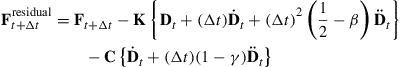
where Fresidual is the residual force vector, and
![]() (3.109)
(3.109)
is defined as the internal force at time t. The acceleration, ![]() , can be simply obtained by
, can be simply obtained by
![]() (3.110)
(3.110)
In practice, the above equation does not usually require the solving of the matrix equation, since lumped masses are usually used which form a diagonal mass matrix (Petyt, 1990). The solution to Eq. (3.110) is thus trivial, and the matrix equation is the set of independent equations for each degree of freedom i as follows:
![]() (3.111)
(3.111)
where ![]() is the residual force, and mi is the lumped mass corresponding to the ith DOF. We now introduce the following finite central difference equations:
is the residual force, and mi is the lumped mass corresponding to the ith DOF. We now introduce the following finite central difference equations:
![]() (3.112)
(3.112)
![]() (3.113)
(3.113)
![]() (3.114)
(3.114)
By eliminating Dt+Δt from Eqs. (3.112) and (3.114), we have
![]() (3.115)
(3.115)
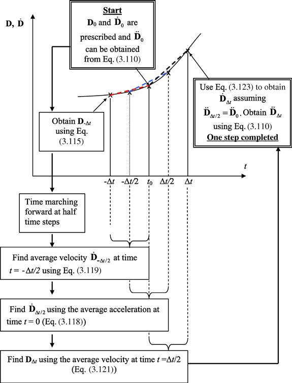
To explain the time stepping procedure, refer to Figure 3.5, which shows an arbitrary plot of either displacement or velocity against time. The time stepping/marching procedure in the central difference method starts at t = 0, and computes the acceleration ![]() using Eq. (3.110):
using Eq. (3.110):
![]() (3.116)
(3.116)
For given initial conditions, D0 and ![]() are known. Substituting D0,
are known. Substituting D0, ![]() , and
, and ![]() into Eq. (3.115), we find
into Eq. (3.115), we find ![]() . Considering a half of the time step and using the central difference Eqs. (3.112) and (3.113), we have
. Considering a half of the time step and using the central difference Eqs. (3.112) and (3.113), we have
![]() (3.117)
(3.117)
![]() (3.118)
(3.118)
The velocity, ![]() at t = −Δt/2 can be obtained by Eq. (3.117) by performing the central differencing at t = −Δt/2 and using values of
at t = −Δt/2 can be obtained by Eq. (3.117) by performing the central differencing at t = −Δt/2 and using values of ![]() and D0:
and D0:
![]() (3.119)
(3.119)
After this, Eq. (3.118) is used to compute ![]() using
using ![]() and
and ![]() :
:
![]() (3.120)
(3.120)
Then, Eq. (3.117) is used once again to compute DΔt using ![]() and D0:
and D0:
![]() (3.121)
(3.121)
Once DΔt is determined, Eq. (3.118) at t = Δt/2 can be used to obtain ![]() by assuming that the acceleration is constant over the step Δt
by assuming that the acceleration is constant over the step Δt
![]() (3.122)
(3.122)
and using ![]() (that is the prescribed initial velocity). We have,
(that is the prescribed initial velocity). We have,
 (3.123)
At the next step in time, ![]() is again computed using Eq. (3.110). The above process is then repeated. The time marching is continued until it reaches the final desired time.
is again computed using Eq. (3.110). The above process is then repeated. The time marching is continued until it reaches the final desired time.
Note that in the above process, the solutions (displacement, velocity, and acceleration) are obtained without solving any matrix form of system equation, but repeatedly using Eqs. (3.110), (3.117), (3.118), and (3.122). The central difference method is therefore an explicit method. The time marching in explicit methods is therefore extremely fast, and the coding is also very straightforward. It is particularly suited for simulating highly nonlinear, large deformation, contact, and extremely fast events of mechanics.
The central difference method, like most explicit methods, is conditionally stable. This means that if the time step, Δt, becomes too large to exceed a critical time step, Δtcr, then the computed solution will become unstable and might grow without limit. The critical time step Δtcr should be the time taken for the fastest stress wave in the solids/structure to across the smallest element in the mesh. Therefore, the time steps used in the explicit methods are typically 100 to 1000 times smaller than those used with implicit methods (that are outlined in the next subsection). The need to use a small time step, and especially its dependence on the smallest element size, makes the explicit codes lose out to implicit codes for some of the problems, especially for those of slow dynamic events.
3.7.2 Newmark’s method (Newmark, 1959)
Newmark’s method is the most widely used implicit algorithm. The example software used in this book, ABAQUS, also uses the Newmark’s method as its implicit solver except that the equilibrium equation defined in Eq. (3.106) is modified with the introduction of an operator defined by Hilber et al. (1978). In this book, we will introduce the standard Newmark’s method as follows. It is first assumed that
![]() (3.124)
(3.124)
![]() (3.125)
(3.125)
where β and γ are constants chosen by the analyst. Equations (3.124) and (3.125) are then substituted into the system equation, Eq. (3.106) to give
 (3.126)
If we group all the terms involving ![]() on the left and shift the remaining terms to the right, we can write
on the left and shift the remaining terms to the right, we can write
![]() (3.127)
(3.127)
![]() (3.128)
(3.128)
and
 (3.129)
The accelerations ![]() can then be obtained by solving the matrix system equation, Eq. (3.127):
can then be obtained by solving the matrix system equation, Eq. (3.127):
![]() (3.130)
(3.130)
Note that the above equation involves matrix inversion, and hence it is analogous to solving a matrix equation. This makes it an implicit method, meaning that one needs to solve a set of linear algebraic equations to obtain a solution at the current time step.
The algorithm normally starts with a prescribed initial velocity and displacements, D0 and ![]() The initial acceleration
The initial acceleration ![]() can then be obtained by substituting D0 and
can then be obtained by substituting D0 and ![]() into Eq. (3.106), if
into Eq. (3.106), if ![]() is not prescribed initially. Then Eq. (3.130) can be used to obtain the acceleration at the next time step,
is not prescribed initially. Then Eq. (3.130) can be used to obtain the acceleration at the next time step, ![]() The displacements
The displacements ![]() and velocities
and velocities ![]() can then be calculated using Eqs. (3.124) and (3.125), respectively. The procedure then repeats to march forward in time until arriving at the final desired time. Because at each time step, the matrix system Eq. (3.127) has to be solved, which can be very time consuming, the implicit algorithm is a very slow time stepping process.
can then be calculated using Eqs. (3.124) and (3.125), respectively. The procedure then repeats to march forward in time until arriving at the final desired time. Because at each time step, the matrix system Eq. (3.127) has to be solved, which can be very time consuming, the implicit algorithm is a very slow time stepping process.
Newmark’s method, like most implicit methods, is unconditionally stable if γ ≥ 0.5 and β ≥ (2γ + 1)2/16. Unconditionally stable methods are those in which the size of the time step, Δt, will not affect the stability of the solution, but rather it is governed by accuracy considerations. The unconditionally stable property allows the implicit algorithms to use significantly larger time steps when the external excitation is of a slow time variation. When the external excitation changes too fast with time, the time step needs to be sufficiently small to capture the time variation features of the excitation.
3.8 Remarks
3.8.1 Summary of shape function properties
The properties of the shape functions are summarized in Table 3.1.
Table 3.1
List of properties of shape functions.
| Item | Name | Significance |
| Property 1 | Reproduction property and consistency | Ensures shape functions produce all the functions that can be formed using basis functions used to create the shape functions. It is useful for constructing shape functions with desired accuracy and consistency in displacement field approximation. |
| Property 2 | Shape functions are linearly-independent | Ensures the shape functions are qualified for a unique approximation of the (displacement) field function. It is often viewed as the default property for any FEM model. |
| Property 3 | Delta function properties | Facilitates an easy imposition of essential boundary conditions. This is a minimum requirement for shape functions workable for the standard FEM. |
| Property 4 | Partitions of unity property | Enables the shape functions to produce the rigid body movements. This is a minimum requirement for shape functions for the standard FEM models. |
| Property 5 | Linear field reproduction | Ensures shape functions produce the linear displacement field. This is a sufficient requirement for shape functions capable of passing the patch test, and hence enabling FEM solution to converge to any smooth displacement solution for solid mechanics problems. |
| Lemma 1 | Condition for shape functions being partitions of unity | Provides an alternative tool for checking the property of partitions of unity of shape functions. |
| Lemma 2 | Condition for shape functions being partitions of unity | Provides an alternative tool for checking the property of partitions of unity of shape functions. |
| Lemma 3 | Condition for shape functions being linear field reproduction | Provides an alternative tool for checking the property of linear field reproduction of shape functions. |
Property 2 is the default property for any FEM model;
Property 3, 4, and 5 are the sufficient requirements for FEM shape functions.
3.8.2 Sufficient requirements for FEM shape functions
Properties 3 and 4 are the minimum requirements for shape functions workable for the FEM. In mesh-free methods (Liu, 2009), Property 3 is not a necessary condition for shape functions. Property 5 is a sufficient requirement for shape functions workable for the FEM for solid mechanics problems. It is possible for shape functions that do not possess Property 5 to produce convergent FEM solutions. In this book, however, we generally require all the FEM shape functions to satisfy Properties 3, 4, and 5. These three requirements are called the sufficient requirements in this book for FEM shape functions; they are the delta function property, partitions of unity, and linear field reproduction.
3.8.3 Recap of FEM procedure
In FEMs, the displacement field U is expressed by displacements at nodes using shape functions defined over elements. Once the shape functions are found, the mass matrix and force vector can be obtained using Eqs. (3.75), (3.78), (3.79), and (3.81). The stiffness matrix can also be obtained using Eq. (3.71), once the shape functions and the strain matrix have been found. Therefore, to develop FE equations for any type of structure components, all one needs to do is formulate the shape function N and then establish the strain matrix B. The other procedures are very much the same. Hence, in the following chapters, the focus will be mainly on the derivation of the shape function and strain matrix for various types of elements for solids and structural components.
3.9 Review questions
1. What is the difference between the strong and weak forms of system equations?
2. What are the conditions that a summed displacement has to satisfy in order to apply the Hamilton’s principle?
3. Briefly describe the standard steps involved in the FEM.
4. Do we have to discretize the problem domain in order to apply the Hamilton’s principle?
5. What is the purpose of dividing the problem domain into elements?
6. For a function defined in [0, l] as
![]()
where l is a given constant, x is an independent variable, and ai (i = 0,1,2) are variable constants (but independent of x). Show that:
a. The variation operator and definite integral operator are exchangeable, i.e.,

b. The variation operator and the differential operator are exchangeable, i.e.,
![]()
7. What are the properties of a shape function? Can we use shape functions that do not possess these properties?

8. Answer the following questions with reference to the two meshes, (a) and (b), shown above:
a. Which mesh will yield more accurate results?
b. Which will be more computationally expensive?
c. Suggest a way of meshing which will yield relatively accurate results and at the same time be less computationally expensive than B?
9. Why is there a need to perform coordinate transformation for each element?
10. Describe how element matrices can be assembled together to form the global system matrix.

11. Consider a 1 DOF system with a rigid block of mass m that can move only in the horizontal direction, as shown in the above figure. The system is at the static equilibrium:
a. Give the expressions for the strain potential energy, work done by external forces, and the total potential energy.
b. Derive the equilibrium equations for the system using the minimum potential energy principle.
c. Show that the total potential energy of the 1DOF system is at a minimum at the equilibrium position.
12. Consider a 1DOF system with a rigid block of mass m that can move only in the horizontal direction, as shown in the previous figure. The system is at a dynamic equilibrium. Derive the dynamic equilibrium equation for this system.

13. Consider a 2DOF system with two rigid blocks that can move only in the horizontal direction, as shown in the above figure. The system is at the static equilibrium:
a. Give the expressions for the strain potential energy, work done by external forces, and the total potential energy.
b. Drive the equilibrium equations for the system using the minimum potential energy principle.
14. Consider again a 2DOF system with two rigid blocks that can move only in the horizontal direction, as shown in the previous figure. The system is at a dynamic equilibrium.
a. Give the expressions for the strain potential energy, work done by external forces, and the total potential energy.
b. Drive the equilibrium equations for the system using the minimum potential energy principle.
15. Consider again the simplest problem of a continuum 1D bar of uniform cross-section, as shown in Figure 2.18. The bar is fixed at the left end and is of length l and section area A. It is subjected to a uniform body force fx and a concentrated force Fs at the right end. The Young’s modulus of the material is E. Using the method of minimum potential energy, obtain the distribution of the displacement for the following cases:
References
1. Crandall SH. Engineering Analysis: A Survey of Numerical Procedures. New York: McGraw-Hill; 1956.
2. Clough RW, Penzien J. Dynamics of Structures. New York: McGraw-Hill; 1975.
3. Finlayson BA. The Method of Weighted Residuals and Variational Principles. New York: Academic Press; 1972.
4. Finlayson BA, Scriven LE. The method of weighted residuals—a review. Applied Mechanics Review. 1966;19:735–748.
5. Hilber HM, Hughes TJR, Taylor RL. Collocation, dissipation and ‘overshoot’ for time integration schemes in structural dynamics. Earthquake Engineering and Structural Dynamics. 1978;6:99–117.
6. Editor-in-chief Kardestuncer H. Finite Element Handbook. McGraw-Hill 1987.
7. Liu GR. Meshfree Methods: Moving Beyond the Finite Element Method. second ed. Boca Raton: CRC Press; 2009.
8. Liu GR, Zhang GY. Smoothed Point Interpolation Methods—G Space Theory and Weakened Weak Forms. New York: World Scientific; 2013.
9. Newmark NM. A method of computation for structural dynamics. ASCE Journal of Engineering Mechanics Division. 1959;85:67–94.
10. Petyt M. Introduction to Finite Element Vibration Analysis. Cambridge: Cambridge University Press; 1990.
11. Reddy JN. Energy and Variational Methods in Engineering. New York: John Wiley; 1984.
12. Washizu K. Variational Methods in Elasticity and Plasticity. second ed. Oxford: Pergamon Press; 1974.
13. Zienkiewicz OC, Taylor RL. The Finite Element Method. fifth ed. Butterworth-Heinemann 2000.