
FEM for Heat Transfer Problems
12.1 Field problems
This chapter introduces the finite element method to solve steady-state heat transfer problems. Many of the materials in this chapter are from the textbook by Segerlind (1984). Heat transfer problems can be categorized generally under one of the many field problems. A field problem is a boundary value problem with the variables (degrees of freedom (DOFs)) described as a varying field in our simulation domain. The distinction here from earlier chapters is that the field is described in a domain comprising of a static mesh—a Eularian mesh. In the earlier chapters, the equations were formulated in a Lagragian mesh, whereby the nodes are displaced according to the calculated displacement and hence the mesh gets deformed. Other common field problems include torsional deformation of bars, irrotational flow, and acoustic problems. This book will make use of the heat transfer problem to introduce the concepts behind the solving of field problems using FEM. Emphasis will be placed on one-dimensional and two-dimensional heat transfer problems. Three-dimensional problems can be solved in similar ways except for the increase in DOFs due to the dependency of field variables on the third dimension. The approach used to derive FE equations in heat transfer problems is a general approach to solve partial differential equations using FEM. Therefore, the FE equations developed for heat transfer problems are directly applicable to all other types of field problems that are governed by similar types of partial differential equations.
The general form of system equations of 2D linear steady-state field problems can be given by the following general form of the Helmholtz equation:
![]() (12.1)
(12.1)
where φ is the field variable, Dx, Dy, g, and Q are given constants whose physical meaning is different for different problems. For one-dimensional field problems, the general form of system equations can be written as
![]() (12.2)
(12.2)
The following subsections introduce different physical problems governed by equations in the form given by Eq. (12.1) or (12.2).
12.1.1 Heat transfer in a two-dimensional fin
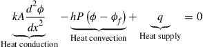
Consider heat transfer in a two-dimensional fin as shown in Figure 12.1. A 2D fin is mounted on a pipe. Heat conduction occurs in the x–y plane, and heat convection occurs on the two surfaces and edges. Assuming that the fin is very thin, so that the temperature does not vary significantly in the thickness (z) direction, therefore the temperature field is only a function of x and y. The governing equation for the temperature field in the fin, denoted by function φ(x, y), can be given by
 (12.3)
where kx and ky are, respectively, the thermal conductivity coefficients in the x and y directions, h is the convection coefficient, t is the thickness of the fin, and φf is the ambient temperature of the surrounding fluid. The heat supply that can be a function of x and y is denoted by q. The governing equation (12.3) can be derived simply by using Fourier’s laws of heat conduction and heat convection, as well as the conservation law of energy (heat). Equation (12.3) simply states that the heat loss due to heat conduction and heat convection should be equal to the heat supply at any point in the fin.

Figure 12.1 A 2D fin mounted on a pipe. Heat conduction occurs in the x–y plane, and heat convection occurs on the two surfaces and edges.
It can be seen that Eq. (12.3) takes on the general form of a field problem as in Eq. (12.1) with the substitution of,
![]() (12.4)
(12.4)
12.1.2 Heat transfer in a long two-dimensional body
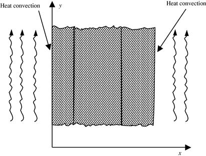
If the domain is elongated in the z direction, and both geometry and temperature do not vary in the z direction, as illustrated in Figure 12.2, then a representative 2D “slice” can be used to model the problem. In this case, there is no heat convection occurring on the two surfaces of the 2D slice, and the governing equation becomes
 (12.5)
which relates to the general form of the field equation with the following substitutions:
![]() (12.6)
(12.6)

12.1.3 Heat transfer in a one-dimensional fin
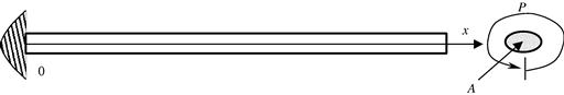
Consider a fin of constant cross-section as shown in Figure 12.3. Assuming that the fin is long and slender, the dimension of the cross-section of the fin is much smaller than the length of the fin. The temperature can be assumed to be constant in the cross-section, and hence it is only a function of x. Heat conduction occurs in the x direction, and heat convection occurs on the circumferential surface of the fin. The temperature field in the fin, denoted by function φ(x), is governed by the following equation
 (12.7)
where k is the thermal conductivity, h is the convection coefficient, A is the cross-sectional area of the fin, and P is the perimeter of the fin, as shown in Figure 12.3. Eq. (12.7) can be derived in the same way as its 2D equivalent in Eq. (12.3). Eq. (12.7) can be written in the general form of Eq. (12.2) with the substitutions of
![]() (12.8)
(12.8)
12.1.4 Heat transfer across a composite wall
Many walls of industrial structures or simple appliances like the thermal flask are composite in nature. They consist of more than one material usually stacked up in layers. By utilizing the thermal conductive properties of the material chosen with a proper stacking sequence, either thermal insulation or effective thermal heat transfer through the walls can be achieved.
Consider the heat transfer across a composite wall as shown in Figure 12.4. The wall is assumed to be infinitely long in the y direction, and hence the heat source and any heat exchanges are also independent of y. In this case, the problem is one-dimensional. Since the wall is infinitely long, it is also not possible to have heat convection along the x axis. Therefore, the system equation in this case is much simpler as compared to that of the fin, and it governs only the heat conduction through the composite wall, which can be given by
 (12.9)
where φ is the known temperature. Eq. (12.9) can be written in a general form of Eq. (12.2) with
![]() (12.10)
(12.10)
12.1.5 Torsional deformation of a bar
For problems of torsional deformation of a bar with noncircular sections, the field variable will be the stress function φ that is governed by a Poisson’s equation,
![]() (12.11)
(12.11)
where G is the shear modulus, and θ is the given angle of twist. The stress function is defined by
 (12.12)
Equation (12.11) can be easily derived in the following procedure.
Consider a pure torsional state where
![]() (12.13)
(12.13)
Therefore, there are only two stress components, σxz and σyz. Using Hooke’s law, we have
 (12.14)
The relationship between displacement and the given angle of twist θ can be given by (Fung, 1965):
![]() (12.15)
(12.15)
Using Eqs. (2.4), (12.15), (12.14), and (12.12) we obtain
![]() (12.16)
(12.16)
![]() (12.17)
(12.17)
Differentiating Eq. (12.16) with respect to y and Eq. (12.17) with respect to x, and equating the two resultant equations, leads to Eq. (12.11).
Once again, it can be seen that Eq. (12.11) takes on the general form of Eq. (12.1) with
![]() (12.18)
(12.18)
12.1.6 Ideal irrotational fluid flow
For problems of ideal, irrotational fluid flow, the field variables are the streamline, ψ, and potential, φ, functions that are governed by the Laplace’s equations,
![]() (12.19)
(12.19)
![]() (12.20)
(12.20)
The derivation of the above equations can be found in any textbook on fluid flows (see, for example, Daily and Harleman, 1966).
It can be seen that both Eqs. (12.19) and (12.20) take on the form of Eq. (12.1) with
![]() (12.21)
(12.21)
12.1.7 Acoustic problems
For problems of a vibrating fluid in a closed volume, as in the case of the vibration of air particles in a room, the field variable, P, is the pressure above the ambient pressure and is governed by the Poisson’s equation,
![]() (12.22)
(12.22)
where w is the wave frequency and c is the wave velocity in the medium. The derivation of the above equations can be found in any book on acoustics (see, for example, Crocker, 1998). It can be seen that Eq. (12.22) takes on the form of Eq. (12.1) with substitutions of
![]() (12.23)
(12.23)
The examples above show that the Helmholtz equation (12.1) governs a wide variety of physical phenomena. Therefore, a productive way to solve all these problems using FEM is to derive FE equations for solving the general form of Eq. (12.1) or (12.2). The following sections will thus introduce FEM as a general numerical tool for solving partial differential equations in the form of Eq. (12.1) or (12.2). We will focus on the application of the FEM to solve heat transfer problems for the rest of the chapter.
12.2 Weighted residual approach for FEM
In Chapter 3, the Hamilton’s principle is used to formulate the FE equations. In that case, one needs to know the functional (the expression of system energy in terms of displacements) for the physical problem. For many engineering problems, one does not know the functional or it is not known as intuitively as in mechanics problems. Instead, the governing equation for the problem would be known. What we want to do now is to establish FEM equations based on the governing equation, but without knowing the functional. For this, it is convenient to use the weighted residual approach to formulate the FEM system equations.
The general form of Eq. (12.1) can be rewritten in the form of
![]() (12.24)
(12.24)
where the function f is given as
![]() (12.25)
(12.25)
In general, it is difficult to obtain the exact solution of φ(x, y) which satisfies Eq. (12.24).
Therefore, an approximated solution of φ(x, y) is sought for, which satisfies Eq. (12.24) in a weighted integral sense, i.e.,
![]() (12.26)
(12.26)
where W is the weight function. By solving for φ(x, y) in Eq. (12.26), we want the solution to be a good approximation to the exact solution of Eq. (12.24). This is the basic idea behind the weighted residual approach. This approach is simple and elegant, and can be used in the finite element method to establish the discretized system of equations as described below.
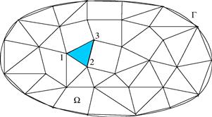
To ensure a good approximation, the problem domain is divided into smaller sub-domains (elements) as we have done in previous chapters, as shown in Figure 12.5. In each element, it is assumed that
![]() (12.27)
(12.27)
where the superscripts indicate that the field variable is approximated, and
![]() (12.28)
(12.28)
in which Ni is the shape function of x and y, and nd is the number of the nodes of the element. For the triangular element shown in Figure 12.5, nd = 3. In Eq. (12.27), Φ(e) is the field variable at the nodes of the element. There are a number of ways in which the weight function, W, can be chosen when developing the element equations. When the shape functions are used as the weight function, the method is called the Galerkin method, which is one of the most popular methods for developing FE equations. The shape function Ni in N is usually developed in exactly the same manner as that discussed in Chapter 3 and other previous chapters. The developed functions should in general satisfy the sufficient conditions discussed in Chapter 3: the delta function property, the partition of unity property, and the linear reproduction property.
Using the Galerkin method, the residual calculated at all the nodes for an element is then evaluated by the following equation.
![]() (12.29)
(12.29)
Finally, the total residual at each of the nodes in the problem domain is then assembled and enforced to zero to establish the system equation for the whole system. FEM equations will be developed in the following sections for one- and two-dimensional field problems, using a heat transfer problem as an example.
12.3 1D heat transfer problem
12.3.1 One-dimensional fin
Consider a one-dimensional fin as shown in Figure 12.6. The governing differential equation for steady-state heat transfer problems for the fin is given by Eq. (12.7). The boundary conditions associated with Eq. (12.7) usually consist of a specified temperature at x = 0
![]() (12.30)
(12.30)
and convection heat loss at the free end where x = H
![]() (12.31)
(12.31)
where φb is the temperature at the end of the fin and is not known prior to obtaining the solution of the problem. Note that the convective heat transfer coefficient in Eq. (12.31) may or may not be the same as the one in Eq. (12.7).

Using the same finite element technique, the fin is divided into elements as shown in Figure 12.6. For each element, the residual equation, R(e) can be obtained using the Galerkin approach as in Eq. (12.29):
 (12.32)
where D = kA, g = hP, and Q = hPφf for heat transfer in thin fins. Note that the minus sign is added to the residual mainly for convenience. Integration by parts is then performed on the first term of the right-hand side of Eq. (12.32), leading to
 (12.33)
Using the usual interpolation of the field variable, φh, by the shape functions in the 1D case,
![]() (12.34)
(12.34)
and substituting Eq. (12.34) into Eq. (12.33), gives
 (12.35)
or
![]() (12.36)
(12.36)
whereby
![]() (12.37)
(12.37)
and is the element matrix of thermal conduction. Matrix ![]() in Eq. (12.36) is defined by
in Eq. (12.36) is defined by
![]() (12.38)
(12.38)
which is the matrix of thermal convection on the circumference of the element. Vector fQ(e) is associated with the external heat applied on the element defined as
![]() (12.39)
(12.39)
Finally, b(e) is defined by
 (12.40)
which is associated with the gradient of the temperature (or heat flux) at the two ends of the element.
In Eq. (12.37), we see the matrix
![]() (12.41)
(12.41)
which is the same as the strain matrix for structural mechanics problems in earlier chapters. For linear elements, the shape functions are as follows:
![]() (12.42)
(12.42)
![]() (12.43)
(12.43)
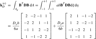
Substituting the above equation into Eq. (12.37), the heat conduction matrix, ![]() , is obtained as
, is obtained as
 (12.44)
The definition of D = kA has been used to derive the above equation. Compared with Eq. (4.15), it is seen that ![]() is in fact an analogy of the stiffness matrix for the 1D truss structure in Chapter 4. The tensile stiffness coefficient
is in fact an analogy of the stiffness matrix for the 1D truss structure in Chapter 4. The tensile stiffness coefficient ![]() has been replaced by the heat conductivity coefficient of
has been replaced by the heat conductivity coefficient of ![]() .
.
Similarly, to obtain the convection matrix ![]() corresponding to the heat convection, substitute Eq. (12.42) in Eq. (12.38),
corresponding to the heat convection, substitute Eq. (12.42) in Eq. (12.38),
 (12.45)
The definition of g = hP has been used to derive the above equation. Compared with Eq. (4.16), it is seen that ![]() is in fact an analogy of the mass matrix of the 1D truss structure. The total mass of the truss element Aρl corresponds to the total heat convection rate of hPl.
is in fact an analogy of the mass matrix of the 1D truss structure. The total mass of the truss element Aρl corresponds to the total heat convection rate of hPl.
The nodal heat vector ![]() is obtained when Eq. (12.42) is substituted into Eq. (12.39), giving
is obtained when Eq. (12.42) is substituted into Eq. (12.39), giving
 (12.46)
The definition of Q = q + hPφf (see, Eq. (12.8)) has been used to derive the above equation. The nodal heat vector consists of the heat supply and the convective heat input to the fin. The nodal heat vector is an analogy of the nodal force vector for the 1D truss element.
Finally, let’s analyze the vector b(e) defined by Eq. (12.40), which is associated with the thermal conditions on the boundaries of the element:
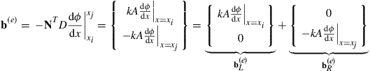 (12.47)
or
![]() (12.48)
(12.48)
where the subscripts “L” and “R” represent the left and right ends of the element. It can be easily proven that at the internal nodes of the fin, ![]() and
and ![]() vanish when the elements are assembled, as illustrated in Figure 12.7. As a result, b needs to be determined only for the nodes on the boundary by using the conditions prescribed. At boundaries where the temperature is prescribed, as shown in Eq. (12.30),
vanish when the elements are assembled, as illustrated in Figure 12.7. As a result, b needs to be determined only for the nodes on the boundary by using the conditions prescribed. At boundaries where the temperature is prescribed, as shown in Eq. (12.30), ![]() or
or ![]() remain an unknown until the full solution is obtained. In fact, it is not necessary to evaluate
remain an unknown until the full solution is obtained. In fact, it is not necessary to evaluate ![]() or
or ![]() while solving the system equation, as the temperature at the node is already known. This situation is very much similar to the prescribed displacement boundary, where the reaction force is usually unknown while solving system equations.
while solving the system equation, as the temperature at the node is already known. This situation is very much similar to the prescribed displacement boundary, where the reaction force is usually unknown while solving system equations.
However, when there is heat convection at the ends of the fin as prescribed in Eq. (12.31), ![]() or
or ![]() is obtained using the boundary conditions, since the heat flux there can be calculated. For example, for boundary conditions defined by Eq. (12.31), we have
is obtained using the boundary conditions, since the heat flux there can be calculated. For example, for boundary conditions defined by Eq. (12.31), we have
 (12.49)
Since φb is the temperature of the fin at the boundary point, we have φb = φj, which is an unknown. Eq. (12.49) can be rewritten as
 (12.50)
or
![]() (12.51)
(12.51)
 (12.52)
and
 (12.53)
Note that Eqs. (12.51), (12.52), (12.53) are derived assuming that the convective boundary is on node j, which is the right side of the element. If the convective boundary is on the left side of the element, we then have
![]() (12.54)
(12.54)
where
 (12.55)
and
 (12.56)
Substituting the expressions for b(e) back to Eq. (12.36), we obtain
 (12.57)
or in a simplified form of
![]() (12.58)
(12.58)
where
![]() (12.59)
(12.59)
and
![]() (12.60)
(12.60)
Note that ![]() and
and ![]() exist only if the node is on the convective boundary, and they are given by Eqs. (12.52) and (12.53) or Eqs. (12.55) and (12.56) depending on the location of the node. If the boundary is insulated, meaning there is no heat exchange occurring there, both
exist only if the node is on the convective boundary, and they are given by Eqs. (12.52) and (12.53) or Eqs. (12.55) and (12.56) depending on the location of the node. If the boundary is insulated, meaning there is no heat exchange occurring there, both ![]() and
and ![]() vanish, because
vanish, because ![]() at such a boundary. After obtaining the element matrices, the residual defined by Eq. (12.58) is assembled and enforced to equate to zero, which will lead to the familiar global system of equations:
at such a boundary. After obtaining the element matrices, the residual defined by Eq. (12.58) is assembled and enforced to equate to zero, which will lead to the familiar global system of equations:
![]() (12.61)
(12.61)
The above matrix equation has the same form as that for a static mechanics problem. The detailed assembly process is described in the examples that follow.
12.3.2 Direct assembly procedure
Consider an element equation of residual in the following form of
![]() (12.62)
(12.62)
or in the expanded form of
 (12.63)
Consider now two linear, one-dimensional elements as shown in Figure 12.8. For element 1,
![]() (12.64)
(12.64)
![]() (12.65)
(12.65)
and for element 2,
![]() (12.66)
(12.66)
![]() (12.67)
(12.67)
The total residual at a node can be obtained by summing all the residuals contributed from all the elements that are connected to the node, and we enforce the total residual to vanish to best satisfy the system equations. We then have at node 1,
![]() (12.68)
(12.68)
at node 2,
![]() (12.69)
(12.69)
and at node 3,
![]() (12.70)
(12.70)
Writing Eqs. (12.68), (12.69), and (12.70) in matrix form gives
 (12.71)
which is the same as the assembly procedure we introduced in Section 3.4.7 of Chapter 3 and Example 4.2 of Chapter 4.

12.3.3 Worked example
We now present a simple case study of a heat transfer problem. The problem is simple, allowing us to explicitly reveal the detailed FEM procedure. For real-life problems, the FEM model can be much bigger, but the essence and basic procedures will largely stay the same. Therefore, a good understanding of this problem and the solution procedure can be beneficial.
Example 12.1
Heat transfer along a 1D fin of rectangular cross-section
The temperature distribution in the fin, shown in Figure 12.9, is to be calculated using the finite element method. The fin is rectangular in shape, 8 cm long, 0.4 cm wide, and 1 cm thick. Assume that convective heat loss occurs from the right end of the fin.
Analysis of the problem: The fin is divided uniformly into 4 elements with a total of 5 nodes. Each element has a length of l = 2 cm. The system equation should be 5 by 5. At node 1 the temperature is specified, therefore there is no need to calculate ![]() and
and ![]() for element 1 as only the temperature is requested. As nodes 2, 3, and 4 are internal, there is also no need to calculate
for element 1 as only the temperature is requested. As nodes 2, 3, and 4 are internal, there is also no need to calculate ![]() and
and ![]() for elements 2 and 3. Since heat convection is occurring on node 5, we have to calculate
for elements 2 and 3. Since heat convection is occurring on node 5, we have to calculate ![]() and
and ![]() using Eqs. (12.52) and (12.53) for element 4.
using Eqs. (12.52) and (12.53) for element 4.
Data preparation:
![]() (12.72)
(12.72)
![]() (12.73)
(12.73)
![]() (12.74)
(12.74)
![]() (12.75)
(12.75)
![]() (12.76)
(12.76)
Solution: The general forms of the element matrices for elements 1, 2, and 3 are
 (12.77)
 (12.78)
Substitute the previously prepared data, Eqs. (12.72), (12.73), (12.74), (12.75), (12.76) into the above two equations, and we have
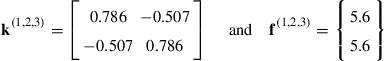 (12.79)
The general forms of the element matrices for element 4 are
 (12.80)
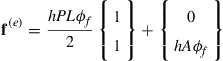 (12.81)
Substituting the data into the above equations, we have
 (12.82)
The next step is to assemble the element matrices together to form the global system of equations. The assembly is carried out using the direct assembly procedure described in the previous section and the resulting global matrix equation is Note that at node 1 the temperature is fixed at a particular value. This requires a heat exchanger (or heat source) there for it to happen. The heat source is unknown at this stage, and it is actually not necessary to know it to compute the temperature distribution. However, it is required for balancing the equation. We therefore simply label it as Q*. Since the temperature at node 1 is given as 80 °C, we actually have four unknown temperatures in a 5 by 5 matrix equation. This implies that we can actually eliminate Q* in the first system equation as indicated below and still solve the four unknowns with the remaining 4 by 4 matrix equation. Note that the term in the second row, first column (circled term) must also be accounted for in the first equation (it is shown below that (–0.507 × φ1) is brought over to the force vector) of the four remaining system equations.
 (12.83)
 (12.84)
Solving the 4 by 4 equation gives the temperature at the nodes:
![]() (12.85)
(12.85)
12.3.4 Remarks
Formulations and examples given in the preceding sections have clearly illustrated that the heat transfer problem is very similar to the structure mechanics problem as far as using the FEM is concerned. The displacement and force correspond to the temperature and heat flux, respectively. We also showed analogies of some of the element matrices and vectors between heat transfer problems and structure mechanics problems. However, we did not mention about the structural mechanics counterparts of the matrix ![]() and vector
and vector ![]() that are coming from the heat convection boundary. Since the heat flux on the boundary depends on the unknown field variable (temperature), the resultant term
that are coming from the heat convection boundary. Since the heat flux on the boundary depends on the unknown field variable (temperature), the resultant term ![]() needs to be combined with the heat convection matrix. In fact, in structure mechanics problems, we can also have a similar situation when the structure is supported by elastic supports such as springs. The reaction force on the boundary depends on the unknown field variable (displacement) at the boundary. For such a system, we will have an additional matrix corresponding to
needs to be combined with the heat convection matrix. In fact, in structure mechanics problems, we can also have a similar situation when the structure is supported by elastic supports such as springs. The reaction force on the boundary depends on the unknown field variable (displacement) at the boundary. For such a system, we will have an additional matrix corresponding to ![]() and a vector corresponding to
and a vector corresponding to ![]() . However, in structure mechanics problems, it is often more convenient to formulate such an elastic support using an additional spring element. The stiffness of the support is then assembled to the global stiffness following the same systematic, direct assembly procedure. The reaction force of the elastic support is found after the global equations system is solved for the displacements.
. However, in structure mechanics problems, it is often more convenient to formulate such an elastic support using an additional spring element. The stiffness of the support is then assembled to the global stiffness following the same systematic, direct assembly procedure. The reaction force of the elastic support is found after the global equations system is solved for the displacements.

We can therefore conclude that the Galerkin residual formulation gives exactly the same FE equations as those we obtained using the energy principles discussed in previous chapters.
12.3.5 Composite wall
Consider heat transfer through a composite wall as shown in Figure 12.10. The governing equation is given by Eq. (12.9). If there is no heat source or sink in a layer (q = 0 within the layer), one linear element is enough for modeling the entire layer. (Why?)1 For the case shown in Figure 12.10, a total of three elements, one for each layer, should be used if there is a heat source within these layers. This argument holds even if there are heat sources or sinks in between the layers.

Figure 12.10 Heat transfer through a composite wall of three layers. One element is sufficient to model a layer if there is no heat supply/sink in the layers.
As for the boundary conditions, at any one or at both outer surfaces, the temperature or heat convection, or heat insulation can be specified. The convective boundary conditions are given as
![]() (12.86)
(12.86)
and
![]() (12.87)
(12.87)
Therefore, all the elements developed in the section for 1D fin are also valid for the case of the composite wall except that ![]() and
and ![]() do not exist because the g and Q vanish in the case of the composite wall (see, Eq. (12.10)).
do not exist because the g and Q vanish in the case of the composite wall (see, Eq. (12.10)).
The general form of the element stiffness matrix is given by
 (12.88)
where ![]() is obtained either by Eq. (12.52) or (12.55), if there is heat convection occurring on the surface, or else
is obtained either by Eq. (12.52) or (12.55), if there is heat convection occurring on the surface, or else ![]() if the surface is insulated. As for a surface with a prescribed temperature, it is not necessary to calculate
if the surface is insulated. As for a surface with a prescribed temperature, it is not necessary to calculate ![]() . For the force vector,
. For the force vector, ![]() , it is obtained either by Eq. (12.53) or (12.56), if there is heat convection occurring on the surface, or zero if the surface is insulated. In the case where the surface has a prescribed temperature, again it is not necessary to have
, it is obtained either by Eq. (12.53) or (12.56), if there is heat convection occurring on the surface, or zero if the surface is insulated. In the case where the surface has a prescribed temperature, again it is not necessary to have ![]() for calculating the temperature. It can always be calculated after the temperature field is found.
for calculating the temperature. It can always be calculated after the temperature field is found.
12.3.6 Worked example
Example 12.2
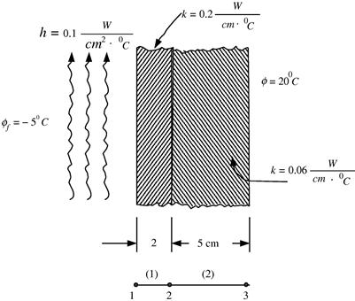
Heat transfer through a composite wall of two layers
Figure 12.11 shows a composite wall consisting of two layers of different materials. Various heat transfer parameters are shown in the figure. The temperature distribution through the composite wall is to be calculated by the finite element method.
Analysis of problem: The wall is divided into 2 elements with a total of 3 nodes. Hence, the global system of equations should be a 3 by 3 matrix equation. At node 3, the temperature is specified, therefore there is no need to calculate ![]() and
and ![]() for element 2. Since the heat convection is occurring on node 1,
for element 2. Since the heat convection is occurring on node 1, ![]() and
and ![]() have to be calculated for element 1 using Eqs. (12.55) and (12.56), respectively.
have to be calculated for element 1 using Eqs. (12.55) and (12.56), respectively.
Data preparation:
For element (1),
![]() (12.89)
(12.89)
![]() (12.90)
(12.90)
![]() (12.91)
(12.91)
For element (2),
![]() (12.92)
(12.92)
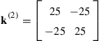
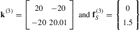
Solution: The element matrices for element (1) are
 (12.93)
The element matrix for element (2) is
 (12.94)
The next step is to assemble the element matrices of the two elements together to form the global system of equations, which leads to the matrix equation:
 (12.95)
Note once again that Q* is still an unknown but is required to balance the equation, as the temperature at node 3 is fixed. Having only two unknown temperatures, φ1 and φ2, the first two equations in the above give
 (12.96)
The above matrix equation (two simultaneous equations with two unknowns) is solved and the solution is given as
![]() (12.97)
(12.97)
Example 12.3
Heat transfer through layers of thin films
Figure 12.12 shows schematically the process of producing layers of thin film of different materials on a substrate using physical deposition techniques. A heat supply is provided on the upper surface of the glass substrate. At the stage shown in Figure 12.12, a layer of iron and a layer of platinum have been formed. The thickness of these layers and the thermal conductivities for the materials of these layers are also shown in Figure 12.12. Convective heat loss occurs on the lower platinum surface, and the ambient temperature is 150 °C. A heat supply is provided to maintain the temperature on the upper surface of the glass substrate at 300 °C. The temperature distribution through the thickness of the thin film layers is to be calculated by the finite element method.
Analysis of problem: This problem is actually similar to the previous example on the composite wall. Hence, 1D elements can be used for this purpose. The layers are divided into 3 elements with a total of 4 nodes as shown in Figure 12.12. Since the temperature is specified at node 1, there is no need to calculate ![]() and
and ![]() for element 1.
for element 1. ![]() and
and ![]() for element 2 are zero since there is no heat convection occurring at either node 2 or 3. Since there is heat convection occurring at node 4,
for element 2 are zero since there is no heat convection occurring at either node 2 or 3. Since there is heat convection occurring at node 4, ![]() and
and ![]() have to be calculated for element 3 using Eqs. (12.55) and (12.56) respectively.
have to be calculated for element 3 using Eqs. (12.55) and (12.56) respectively.
Data preparation:
For element (1),
![]() (12.98)
(12.98)
For element (2),
![]() (12.99)
(12.99)
For element (3),
![]() (12.100)
(12.100)
![]() (12.101)
(12.101)
![]() (12.102)
(12.102)
Solution: The element matrix for element (1) is
 (12.103)
The element matrix for element (2) is
 (12.104)
And finally the element matrices for element (3) are
 (12.105)
The next step is to assemble the element matrices of the three elements together to form the global system equations, which leads to
 (12.106)
Since φ1 is given to be 300 °C, we can therefore reduce the above equation to a 3 x 3 matrix to solve for the remaining 3 unknown temperatures
 (12.107)
The above matrix equation is solved and the solution can be obtained as:
![]() (12.108)
(12.108)
To calculate the heat flux, Q* on the top of the glass substrate, we can now substitute the temperatures into the first equation of the matrix equation in Eq. (12.106) to obtain
![]() (12.109)
(12.109)
12.4 2D heat transfer problem
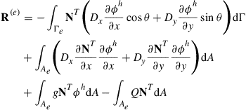
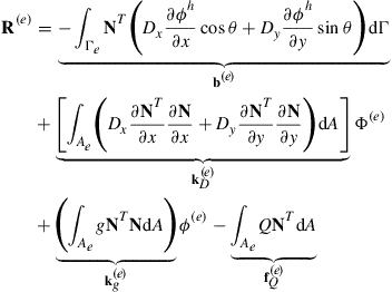
12.4.1 Element equations
This section deals with heat transfer problems in 2D that is governed by Eq. (12.1). The procedure for obtaining the FEM equations for 2D heat transfer problems is the same as that for the 1D problems described in the previous sections, except that the mathematical manipulation becomes slightly more involuted due to the additional dimension.

Let us assume that the problem domain is divided into elements as shown in Figure 12.5. For one element in general, the residual can be obtained by the Galerkin method as
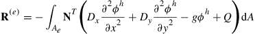 (12.110)
Note that the minus sign is added to the residual mainly for convenience and has no consequence for the end result since we eventually enforce the residual to zero. The integration in Eq. (12.110) for the residual must be evaluated so as to obtain the element matrices, but in this case, the integration is more complicated than the 1D case because the integration is performed over the area of the element. Recall that in the 1D case, the integral is evaluated by parts. In the 2D case, we need to use the Gauss’s divergence theorem instead.
First, using the product rule for differentiation, the following expression can be obtained:
![]() (12.111)
(12.111)
The first integral in Eq. (12.110) can then be obtained by
![]() (12.112)
(12.112)
where Ae is the area of the element. Gauss’s divergence theorem can be stated mathematically for this case as
![]() (12.113)
(12.113)
where θ is the angle of the outwards normal on the boundary Γe of the element with respect to the x axis. Eq. (12.113) is thus substituted into Eq. (12.112) to obtain
![]() (12.114)
(12.114)
In a similar way, the second integral in Eq. (12.110) can be evaluated to obtain
![]() (12.115)
(12.115)
The two integrals in Eqs. (12.114) and (12.115) are substituted back into the residual in Eq. (12.110) to give
 (12.116)
The field variable φ is now interpolated from the nodal variables by shape functions as in Eq. (12.34), which is then substituted into Eq. (12.116) above to give
 (12.117)
or in matrix form of
![]() (12.118)
(12.118)
where
 (12.119)
 (12.120)
![]() (12.121)
(12.121)
![]() (12.122)
(12.122)
Like in the 1D case, the vector b(e) is related to the variation or the derivatives of temperature (heat flux) on the boundaries of the element. It will be evaluated in detail in the next section. For now, let us evaluate and analyze Eqs. (12.120), (12.121), (12.122).
The integral in Eq. (12.120) can be rewritten in the matrix form by defining
 (12.123)
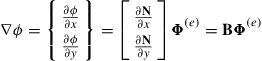 (12.124)
where B is the strain matrix given by
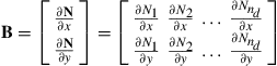 (12.125)
Note that we use the usual shape function given by Eq. (12.28) to obtain the above equations. Using Eqs. (12.123), (12.124), (12.125), it can be easily verified that
![]() (12.126)
(12.126)
Therefore, the general element “stiffness” matrix for 2D elements given by Eq. (12.120) becomes
![]() (12.127)
(12.127)
which is exactly the same form as Eq. (3.71) that is obtained using the Hamilton’s principle, except that the matrix of material elasticity is replaced by the matrix of heat conductivity. Note also that in Eq. (12.121), ![]() is similar to the matrix given by Eq. (3.75) for mechanics problems. We observe once again that the Galerkin weighted residual formulation produces the same set of FE equations as those produced by the energy principle.
is similar to the matrix given by Eq. (3.75) for mechanics problems. We observe once again that the Galerkin weighted residual formulation produces the same set of FE equations as those produced by the energy principle.
12.4.2 Triangular elements
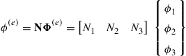
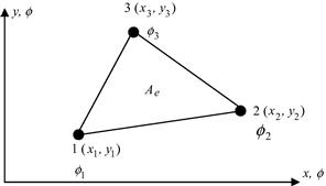
Using shape functions of the 2D triangular element, the field function of temperature, φ, can be interpolated as follows:
 (12.128)
where Ni (i = 1, 2, 3) are the three shape functions defined by Eq. (7.22) and (7.23), and φi (i = 1, 2, 3) are the nodal values of temperature at the 3-nodes of the triangular element shown in Figure 12.13.
Note that the strain matrix B is constant for triangular elements, and can be evaluated similar to Eq. (7.38). Using Eq. (12.127), ![]() can be easily evaluated as the integrand and is a constant matrix if the material constants Dx and Dy do not change within the element.
can be easily evaluated as the integrand and is a constant matrix if the material constants Dx and Dy do not change within the element.
![]() (12.129)
(12.129)
Expanding the matrix product yields
 (12.130)
It is noted that the stiffness matrix is symmetrical.
The matrix, ![]() defined by Eq. (12.121) can be evaluated as
defined by Eq. (12.121) can be evaluated as
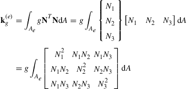 (12.131)
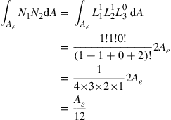
The above integral can be carried out using the factorial formula given in Eq. (7.43), since the shape functions are equal to the area coordinates—just as we did for the mass matrix, Eq. (7.44), in Chapter 7. For example,
 (12.132)
Using the area coordinates and the factorial formula in Eq. (7.43), the matrix ![]() is found as
is found as
 (12.133)
The element force vector ![]() defined in Eq. (12.122) also involves the integration of shape functions and can also be obtained using the factorial formula in Eq. (7.43):
defined in Eq. (12.122) also involves the integration of shape functions and can also be obtained using the factorial formula in Eq. (7.43):
 (12.134)
It is assumed that Q is a constant within the element. Note that the heating rate, QA, is equally shared by the three nodes of the triangular element.
12.4.3 Rectangular elements
Consider now a 4-nodal, rectangular element as shown in Figure 7.8. The field function φ is interpolated over the element as follows.
 (12.135)
Note that for rectangular elements, the natural coordinate system is again adopted as for the case in structure mechanics problem, as shown in Figure 7.8. The shape functions are given by Eq. (7.51) and are known as bilinear shape functions. The strain matrix for the rectangular element can be evaluated in a form similar to Eq. (7.55). Note that for bilinear elements, the strain matrix is no longer constant. Using Eqs. (12.127) and (7.51) ![]() can be evaluated as
can be evaluated as
 (12.136)
The matrix ![]() defined by Eq. (12.121) can be evaluated as
defined by Eq. (12.121) can be evaluated as
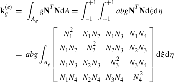 (12.137)
which results in
 (12.138)
The element force vector, ![]() , defined in Eq. (12.122) also involves the integration of the shape functions and with the substitution of the shape functions in Eq. (7.51), it can be obtained as
, defined in Eq. (12.122) also involves the integration of the shape functions and with the substitution of the shape functions in Eq. (7.51), it can be obtained as
 (12.139)
Note that in the above, Q is assumed to be constant within the element. The heating rate, QA, is equally shared by the four nodes of the rectangular element.
In this subsection, matrices ![]() have been evaluated exactly and explicitly for rectangular elements. In engineering practice, however, it is very rare to use rectangular elements unless the geometry of the problem domain is also a rectangular one. Very often, the more general, quadrilateral elements with four nodes and four non-parallel sides are used to mesh the problem domain defined by a complex geometry. Formulating FEM equations for quadrilateral elements has been detailed in Section 7.4. Note that with quadrilateral elements, it is difficult to work out the exact explicit form of the element matrices. Therefore, the integrals are carried out in most of the commercial software packages using numerical integral schemes such as the Gauss integration scheme discussed in Chapter 7 for 2D solid elements.
have been evaluated exactly and explicitly for rectangular elements. In engineering practice, however, it is very rare to use rectangular elements unless the geometry of the problem domain is also a rectangular one. Very often, the more general, quadrilateral elements with four nodes and four non-parallel sides are used to mesh the problem domain defined by a complex geometry. Formulating FEM equations for quadrilateral elements has been detailed in Section 7.4. Note that with quadrilateral elements, it is difficult to work out the exact explicit form of the element matrices. Therefore, the integrals are carried out in most of the commercial software packages using numerical integral schemes such as the Gauss integration scheme discussed in Chapter 7 for 2D solid elements.
12.4.4 Boundary conditions and vector b(e)
Previously, it is mentioned that the vector, b(e), for the 2D element as defined by Eq. (12.119) is associated with the variation or derivatives of temperature (or heat flux) on the boundaries of the element. In this section, the relationship of the vector, b(e), with the boundaries of the element, and hence the boundaries of the problem domain, will be studied in detail.
The vector b(e) defined in Eq. (12.119) is first split into two parts:
![]() (12.140)
(12.140)
where ![]() comes from integration of the element boundaries lying inside the problem domain, and
comes from integration of the element boundaries lying inside the problem domain, and ![]() is that which lies on the boundary of the problem domain. It can then be proven that
is that which lies on the boundary of the problem domain. It can then be proven that ![]() should vanish, which we have seen for the one-dimensional case.
should vanish, which we have seen for the one-dimensional case.
Figure 12.14 shows two adjacent elements numbered, 1 and 2. In evaluating the vector, b(e), as defined in Eq. (12.119), the integration needs to be done on all the edges of these elements. As Eq. (12.119) involves a line integral, the results will be direction-dependent. The direction of integration has to be consistent for all the elements in the system, either clockwise or counter-clockwise. For elements 1 and 2, their directions of integration are assumed counter-clockwise as shown by arrows in Figure 12.14. Note that on their common edge j-k the value of ![]() obtained for element 2 is the same as that obtained for element 1, except that their signs are opposite because the directions of integration on this common edge for both elements are opposite. Therefore, when these elements are assembled together, values of
obtained for element 2 is the same as that obtained for element 1, except that their signs are opposite because the directions of integration on this common edge for both elements are opposite. Therefore, when these elements are assembled together, values of ![]() will cancel each other out and vanish. This happens for all other element edges that fall in the interior of the problem domain. Obviously, when the edge lies on the boundary of the problem domain (where it is not shared),
will cancel each other out and vanish. This happens for all other element edges that fall in the interior of the problem domain. Obviously, when the edge lies on the boundary of the problem domain (where it is not shared), ![]() has to be evaluated.
has to be evaluated.

Figure 12.14 Direction of integration path for evaluating b(e). For element edges that are located in the interior of the problem domain, b(e) vanishes after assembly of the elements, because the values of b(e) obtained for the same edge of the two adjacent elements possess opposite signs.
The boundary of the problem domain can be divided broadly into two categories. One is the boundary where the field variable temperature φ is specified, as noted by Γ1 in Figure 12.15, which is known as the essential boundary condition. The other is the boundary where the derivatives of the field variable of temperature (heat flux) are specified, as shown in Figure 12.15. This second type of boundary condition is known as the natural boundary condition. For the essential boundary condition, we do not need to evaluate ![]() at the stage of formulating and solving the FEM equations, as the temperature is already known, and the corresponding columns and rows will be removed from the global FEM equations in order to solve for the other unknowns. We have seen such a treatment in examples such as Example 12.1. Because b(e) is derived naturally from the weighted residual weak form, it is termed the natural boundary condition. Therefore, our concern is only for elements that are on the natural boundaries, where the derivatives of the field variable are specified, and special methods of evaluating the integral are required just as in the 1D case (Example 12.2).
at the stage of formulating and solving the FEM equations, as the temperature is already known, and the corresponding columns and rows will be removed from the global FEM equations in order to solve for the other unknowns. We have seen such a treatment in examples such as Example 12.1. Because b(e) is derived naturally from the weighted residual weak form, it is termed the natural boundary condition. Therefore, our concern is only for elements that are on the natural boundaries, where the derivatives of the field variable are specified, and special methods of evaluating the integral are required just as in the 1D case (Example 12.2).

Figure 12.15 Types of boundary conditions. Γ1: Essential boundary where the temperature is known; Γ2: Natural boundary where the heat flux (derivative of temperature) is known.
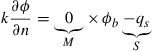
In problems of heat transfer, natural boundary often refers to a boundary where heat convection occurs. The integrand in Eq. (12.119) can be generally rewritten in the following form:
![]() (12.141)
(12.141)
where θ is the angle of the outwards normal on the boundary with respect to the x axis, M and S are given constants depending on the type of the natural boundaries, and φb is the unknown temperature on the boundary. Note that the left-hand side of Eq. (12.141) is in fact the heat flux across the boundary, and can therefore be rewritten as
![]() (12.142)
(12.142)
where k is the heat conductivity at the boundary point in the direction of the boundary normal. For heat transfer problems, there are the following types of boundary conditions:
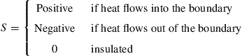
Heat Insulation boundary: On the boundary where the heat is insulated from heat exchange, there will be no heat flux across the boundary and the derivatives of temperature there will be zero. In such cases, we have M = S = 0, and the value of ![]() is simply zero.
is simply zero.
Convective boundary condition:Figure 12.16 shows the situations whereby there are exchanges of heat via convection. Following the Fourier’s heat convection law, the heat flux across the boundary due to the heat conduction can be given by
![]() (12.143)
(12.143)
where k is the heat conductivity at the boundary point in the direction of the boundary normal. On the other hand, following Fourier’s heat convection law, the heat flux across the boundary due to the heat convection can be given by
![]() (12.144)
(12.144)
where h is the heat convection coefficient at the boundary point in the direction of the boundary normal. At the same boundary point the heat flux by conduction should be the same as that by convection, i.e, qk = qh, which leads to
 (12.145)
The values of M and S for heat convection boundary are then found to be
![]() (12.146)
(12.146)
Specified heat flux on boundary: When there is a heat flux specified on the boundary as shown in Figure 12.17. The heat flux across the boundary due to the heat conduction can be given by Eq. (12.143). The heat flux by conduction should be the same as the specified heat flux, i.e, qk = qs, which leads to
 (12.147)
The values of M and S for heat convection boundary are then found to be
![]() (12.148)
(12.148)
From Figure 12.17, it can be seen that
 (12.149)
For other cases whereby M and/or S is not zero, ![]() can be given by
can be given by
 (12.150)
where φb can be expressed using shape function as follows
![]() (12.151)
(12.151)
Substituting Eq. (12.151) back into Eq. (12.150) leads to
 (12.152)
or
![]() (12.153)
(12.153)
in which,
![]() (12.154)
(12.154)
is the contribution by the natural boundaries to the “stiffness” matrix, and
![]() (12.155)
(12.155)
is the force vector contribution from the natural boundaries.


Let us now calculate the force vector ![]() for a rectangular element shown in Figure 7.8. Assuming that S is specified over side 1–2,
for a rectangular element shown in Figure 7.8. Assuming that S is specified over side 1–2,
 (12.156)
where the shape functions are given by Eq. (7.51) in the natural coordinate system. Note, however, that N3 = N4 = 0 along edge 1–2. Substituting the nonzero shape functions into the above equation, we obtain
 (12.157)
The above equation implies that the quantity of (2aS) is shared equally between the two nodes 1 and 2 on the edge. This even distribution among the nodes on the edge is valid for all the elements with linear shape function. Therefore, if the natural boundary is on the other three edges of the rectangular element, the force vector can be simply written as follows:
 (12.158)
Note that if S is specified on more than one side of an element, the values for ![]() for the appropriate sides are added together.
for the appropriate sides are added together.
The same principle of equal sharing can be applied to the linear triangular element shown in Figure 12.13. The expression for the force vectors on the three edges can be simply written as
 (12.159)
The quantities L12, L23, and L13 are the lengths of the respective edges of the triangular element.
Using Eq. (12.154) to derive ![]() for the rectangular element shown in Figure 7.8, we obtain
for the rectangular element shown in Figure 7.8, we obtain
 (12.160)
Note that the line integration is performed round the edge of the rectangular element. If we assume that M is specified over edge 1–2, then N3 = N4 = 0 and the above equation becomes
 (12.161)
Evaluation of the individual coefficients after noting that η = −1 for edge 1–2 gives
 (12.162)
Eq. (12.161) thus becomes
 (12.163)
It is observed that the amount of (2aM) is shared by four components k11, k12, k21, and k22 in ratios of ![]() , and
, and ![]() . This sharing principle can be used to obtain the matrices
. This sharing principle can be used to obtain the matrices ![]() directly for situations where M is specified on the other three edges. They are
directly for situations where M is specified on the other three edges. They are
 (12.164)
This sharing principle can also be applied to linear triangular elements, since the shape functions are also linear, and the corresponding matrices are:
 (12.165)

12.4.5 Point heat source or sink
If there is a heat source or sink in the domain of the problem, it is best recommended in the modeling that a node is placed at the point where the source or sink is located, so that the source or sink can be directly added into the force vector, as shown in Figure 12.18. If, for some reason, this cannot be done, then we have to distribute the source or sink to the nodes of the element in which the source or sink is located. To do this, we have to go back to Eq. (12.122), which is once again rewritten below
![]() (12.166)
(12.166)
Consider a point source or sink in a triangular element as shown in Figure 12.19. The source or sink can be mathematically expressed using delta functions
![]() (12.167)
(12.167)
where Q* represents the strength of the source or sink, and (X0, Y0) is the location of the source or sink. Substitute Eq. (12.167) into Eq. (12.166) and we obtain
 (12.168)
which becomes
 (12.169)
This implies that the source or sink is shared by the nodes of the elements in the ratios of shape functions evaluated at the location of the source or sink. This sharing principle can be applied to any type of elements, and also other types of physical problems, for example, a concentrated force applied in the middle of a 2D element.

12.5 Summary
Finite element formulation for field problems that are governed by the general form of Helmholtz equation can be summarized as follows.

12.6 Case study: Temperature distribution of heated road surface
Figure 12.20 shows the cross-section of a road with heating cables to prevent the surface of the road from freezing. The cables are 4 cm apart and 2 cm below the surface of the road. The slab rests on a thick layer of insulation and the heat loss from the bottom can be neglected. The conductivity coefficients are kx = ky = 0.018 W/cm°C and the surface convection coefficient is h = 0.0034 W/cm°C. The latter corresponds to about a 30–35 km/hr of wind velocity. The surface temperature of the road is to be determined when the cable produces 0.080 W/cm of heat and the air temperature is −6 °C.

12.6.1 Modeling
Since the road is very long in the horizontal direction, a representative section shown in Figure 12.20 can be used to model the entire problem domain. The FE mesh is shown in Figure 12.21 together with boundary conditions specified.

The mesh shown in Figure 12.21 demonstrates mesh transition from an area consisting of a sparse mesh to an area of denser mesh. The analyst has chosen to mesh it this way since the temperature distribution at the bottom of the model is not critical. Hence, computational time is reduced as a result. The transition is done with the use of triangular elements in between larger rectangular elements and smaller rectangular elements. Note that all the elements used are linear elements and hence the mixture of elements here is compatible.
12.6.2 ABAQUS input file
Part of the ABAQUS input file is shown here:


The information provided in the above input file is being used by the software in a similar manner as that discussed in the previous case studies in previous chapters.
12.6.3 Results and discussion
Running the above problem in ABAQUS, the nodal temperatures can be calculated. Figure 12.22 shows a fringe plot of the distribution of the temperatures in the model. It can be seen clearly how the temperature varies from a maximum at the heat source (the heating cables) to other parts of the road cross-section.

In the analysis, the temperatures at all the nodes are calculated. For this problem, we would be interested in only the temperature of the road surface. Table 12.1 shows the nodal temperature on the surface of the road. It can be seen here how the presence of the heating cables under the road is able to keep the road surface at a temperature above the freezing point of water (0 °C). This would prevent the build-up of ice on the road surface during winter, which makes it safer for drivers on the road. The usefulness of the finite element method is demonstrated here as there are actually many parameters involved when it comes to designing such a system. For example, how deep should the cables be buried underground, what should be the distance between cables, what is the amount of heat generated by the heating cables that is sufficient for the purpose, and so on. The finite element method used here can effectively aid the engineer in deciding all these parameters.
12.7 Review questions
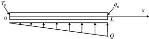
1. a. A fin with a length L has a uniform cross-sectional area A and thermal conductivity k as shown in Figure 12.23. A linearly distributed heat supply is applied on the fin. The temperature at the left end is fixed at T0, and the heat flux at the right end is q0. The governing equation for the fin is given by
![]()
Develop the finite element equation for a TWO-node element.
b. If L = 8 m, A = 1 m2, k = 5 J/°Cms, Q = 100 J/sm, T0 = 0, and q0 = 15 J/m2s, determine the temperatures at the nodes by using two linear elements.
2. Figure 12.24 shows a one-dimensional fin of length L and a varying cross-sectional area A(x). The thermal conductivity of the material that is constant is denoted by k. Heat convection occurs on the surfaces of the fin, and the ambient temperature is denoted by Tf. The governing equation for the temperature T in the fin is given by
![]()
where h is a given convection coefficient. The area of the fin is given by
![]()
where A0 and Ad are constants. The circumference of the cross-section of the fin is given by
![]()
where P0 and Pd are constants.
Develop the finite element equations for a two-node linear element of length L.

3. Figure 12.25 shows a sandwiched composite wall. Convection heat loss occurs on the left surface, and the temperature on the right surface is constant. Considering a unit area, and with the parameters given in Figure 12.25, use three linear elements (one for each layer) to:
a. determine the temperature distribution through the composite wall, and
b. calculate the flux on the right surface of the wall.

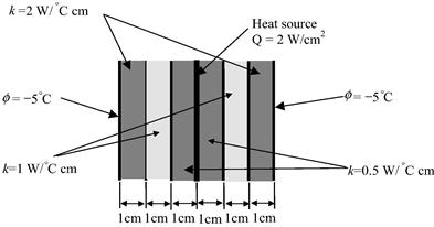
4. Figure 12.26 shows a system of a composite wall. The temperature of the two outer surfaces of the wall is kept constant. A heat source is located in the middle surface of the wall. Using linear elements:
a. determine the temperature distribution across the composite wall,
b. calculate the flux on the surfaces of the wall,
c. calculate the temperature distribution across the wall, when φ = −2.5 °C while all other parameters remain the same, and
d. explain whether or not higher order elements lead to more accurate results.
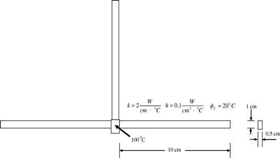
5. Figure 12.27 shows an array of identical fins with square cross-section used to dissipate the heat of two vertical walls connected to these fins. At the steady-state, the temperature on these walls is kept at 100 °C. The dimensions and the thermal conductivity of the fins, the convection coefficient on the surfaces of the fine, and the ambient temperature are given in the figure.
a. Using four linear elements for each fin, determine the temperature distribution along the fins.
b. Calculate all the heat dissipated by each of the fins.
c. Is the FEM capable of producing the exact solution? Justify your answer.
d. What is the possible ways to improve the accuracy of the solution? Which way is the most preferred?

Figure 12.27 An array of identical fins with square cross-section used to dissipate the heat of two vertical walls connected to these fins.
6. Consider a soldering situation where the tip raises the temperature at point A of a copper wire to 100 °C, shown in Figure 12.28. The wire is 15 cm long and 0.02 cm in diameter. The temperature at both ends is 20 °C. The thermal conductivity k of the copper wire is 26 J/°Cms. Assume the circumferential surface of the wire is adiabatic. Using three linear elements of equal length,
a. determine the heat flux into the wire at point A,
b. determine the heat flux at both ends of the wire,
c. explain whether three elements are really needed for this problem, and
d. repeat (b) for a given heat flux of 4 × 10⁻³ J/s instead of the temperature.

7. Consider a quadratic heat-conduction line element with 3 equally spaced nodes as shown in Figure 12.29.
a. Using the quadratic element, determine the heat conduction matrix.
b. Using one linear element for the left portion, and one quadratic element for the right portion of the wire shown in Figure 12.28 of question 5 above, determine the heat flux at point A and both ends of the wire.
c. Comment on the results by comparing them with the results of question 3.

8. Figure 12.30 shows three identical fins used to dissipate the heat. At the steady state, the temperature at the roots of these three fins is kept at 100 °C.
a. Using two linear elements for each fin, determine the temperature distribution along all three fins.
b. Calculate all the heat dissipated by all three fins.
c. Explain how many elements in a fin are required to obtain an accurate solution. What is the other way to improve the accuracy of the solution without increasing the number of elements? Which way is more efficient?
References
1. Segerlind LJ. Applied Finite Element Analysis. 2nd ed. John Wiley & Sons, Inc. 1984.
2. Daily JW, Harleman DRF. Fluid Dynamics. Reading, Mass: Addison-Wesley; 1966.
3. Crocker MJ, ed. Handbook of Acoustics. John Wiley & Sons 1998; Chapter 1.
4. Fung YC. Foundations of Solid Mechanics. Englewood Cliffs: Prentice-Hall; 1965.
1Hint: see Example 4.1.