FEM for Two-Dimensional Solids
7.1 Introduction
In this chapter, we develop finite element (FE) equations for the stress analysis of two-dimensional (2D) solids subjected to external loads. The basic concepts, procedures, and formulations can also be found in many existing textbooks (see Zienkiewicz and Taylor, 2000). The element developed here is called a 2D solid element that is used for solid mechanics problems where the loading (and hence the deformation) occur only within a plane. Though no real life structure can be truly 2D, experienced analysts can often idealize many 3D practical problems to 2D problems with satisfactory results by carrying out analyses using 2D models, which are usually much more efficient and cost effective compared to conducting full 3D analyses. As discussed in Chapter 2, there are 2D plane stress and plane strain problems, whereby correspondingly, plane stress and plane strain elements need to be used to solve them. For example, if we have a plate structure with loading acting in the plane of the plate as in Figure 7.1, we need to use 2D plane stress elements. When we want to model the effects of water pressure on a dam, as shown in Figure 7.2, we have to use 2D plane strain elements to model just the cross-section.


Note that in Figure 7.1, plane stress conditions are usually applied to structures that have relatively small thickness as compared to their other dimensions. Due to the absence of any off-plane external force, the normal stresses are negligible, which leads to a plane stress situation. In cases where plane strain conditions are applied, as in Figure 7.2, the thickness of the structure (in the z direction) is relatively large as compared to its other dimensions, and the loading (pressure) is uniform along the elongated direction. The deformation is, therefore, approximated to be the same throughout its thickness. In this case, the off-plane strain (strain components in the z direction) is negligible, which leads to a plane strain situation. In either a plane stress or plane strain situation, the governing system equation can be drastically simplified, as shown in Chapter 2. The formulations for plane stress and plane strain problems are very much the same, except for the difference in the material constant matrix. Another often encountered 2D problem comes from simplification of axisymmetric structures, which will also be discussed in this chapter.
A 2D solid element, be it plane strain or plane stress, can be triangular, rectangular or quadrilateral in shape with straight or curved edges. The most often used elements in engineering practice are linear elements (and thus with straight edges). Quadratic elements are also used for situations that require higher accuracy in stress, but they are less often used for practical problems. Higher order elements have also been developed, but they are generally less often used except for certain specific problems. The order of the 2D element is determined by the order of the shape functions used. A linear element uses linear shape functions, and therefore the edges of the element are straight. A quadratic element uses quadratic shape functions, and their edges can be curved. The same can be said for elements of the third order or higher.
In a 2D model, the elements can only deform in the plane where the model is defined, and in most situations, this is taken to be the x–y plane. At any point, the variable, that is the displacement, has two components in the x and y directions, and so do the external forces. For plane strain problems, the thickness of the true structure is usually not important, and is normally treated as a unit quantity uniformly throughout the 2D model. However, for plane stress problems, the thickness is an important parameter for computing the stiffness matrix and stresses. Throughout this chapter, it is assumed that the elements have a uniform thickness of h. If the structure to be modeled has a varying thickness, the structure needs to be divided into small elements, where, in each element, a uniform thickness can be used. On the other hand, formulation of 2D elements with varying thicknesses can also be done easily, as the procedure is similar to that of a uniform element. However, very few commercially available software packages provide elements of varying thickness.
The equation system for a 2D element will be more complex as compared with the 1D element because of the higher dimension. The procedure for developing these equations is, however, very similar to that for the 1D truss elements, which is detailed in Chapter 4. These steps can be summarized in the following three-step procedure:
1. Construction of shape functions matrix N that satisfies Eqs. (3.34) and (3.41).
2. Formulation of the strain matrixB.
3. Calculation of ke,me, and fe using N and B and Eqs. (3.71), (3.75), and (3.81).
We shall be focusing on the formulation of three types of simple but very important elements: linear triangular, bilinear rectangular, and isoparametric linear quadrilateral elements. Once the formulation of these three types of element is understood, the development of other types of elements of higher orders is straightforward, because the same techniques can be utilized. Development of higher order elements will be discussed at the end of this chapter.
7.2 Linear triangular elements
The linear triangular element was the first type of element developed for 2D solids. The formulation is also the simplest among all the 2D solid elements. It has been found that the linear triangular element is less accurate compared to bilinear quadrilateral elements. For this reason, it is often thought to be ideal to use quadrilateral elements, but the reality is that the triangular element is still a very useful element for its adaptation to complex geometry. Triangular elements are normally used when we want to mesh a 2D model involving complex geometry with acute corners. Most importantly, the triangular configuration with the simplest topological feature makes it easier to develop automated meshing processors. Nowadays, analysts are hoping to use a fully automated mesh generator to perform the complex task of analysis that needs repeated or even adaptive re-meshing. Most automated mesh generators can only create triangular elements. There are automated mesh generators that can generate a quadrilateral mesh, but they still use triangular elements as patches for complex geometry, and end up with a mesh of mixed elements. Hence, despite being less accurate, we still have to use triangular elements for many practical engineering problems.
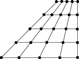
Consider a 2D model in the x–y plane, shown schematically in Figure 7.3. The 2D domain is divided in a proper manner into a number of triangular elements. The “proper” meshing of a domain will be outlined in Chapter 11, where a list of guidelines is provided. In a mesh of linear triangular elements, each triangular element has three nodes and three straight edges.

7.2.1 Field variable interpolation
Consider now a triangular element of uniform thickness h. The nodes of the element are numbered 1, 2, and 3 counter-clockwise, as shown in Figure 7.4. For 2D solid elements, the field variable is the displacement, which has two components (u and v), and hence each node has two degrees of freedom (DOFs). Since a linear triangular element has three nodes, the total number of DOFs of a linear triangular element is six. For the triangular element, the local coordinate of each element can be taken as the same as the global coordinate, since there is no advantage in specifying a different local coordinate system for each element.

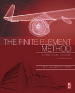
Now, let’s examine how a triangular element can be formulated. The displacement U is generally a function of the coordinates x and y, and we express the displacement at any point in the element using the displacements at the nodes and shape functions. It is therefore assumed that (see Section 3.4.2)
![]() (7.1)
(7.1)
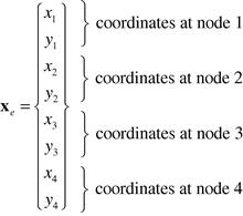
where the superscript h indicates that the displacement is approximated, and de is a vector of the nodal displacements arranged in the order of
 (7.2)
(7.2)
and the matrix of shape functions N is arranged as
 (7.3)
(7.3)
in which Ni (i = 1, 2, 3) are three shape functions corresponding to the three nodes of the triangular element. Equation (7.1) was written in a compact matrix form, which can be explicitly expressed as
 (7.4)
(7.4)
which implies that each of the displacement components at any point in the element is approximated by an interpolation from the nodal displacements using the shape functions. This is because the two displacement components (u and v) are basically independent from each other. The question now is how we can construct the shape functions, Ni, for our triangular element that satisfies the sufficient requirements: delta function property; partitions of unity; and linear field reproduction.
7.2.2 Shape function construction
Development of the shape functions is normally the first, and most important, step in developing FE equations for any type of element. In determining the shape functions Ni (i = 1, 2, 3) for the triangular element, we can of course follow exactly the standard procedure described in Sections 3.4.3 and 4.2.1, by starting with an assumption of the displacements using polynomial basis functions with unknown constants. These unknown constants are then determined using the nodal displacements at the nodes of the element. This standard procedure works in principle for the development of any type of element, but may not be the most convenient method. We demonstrate here another slightly different approach for constructing shape functions. We start with an assumption of shape functions directly using polynomial basis functions with unknown constants. These unknown constants are then determined using the property of the shape functions. The only difference here is that we assume the shape function in a polynomial form instead of assuming the displacements. For a linear triangular element, we assume that the shape functions are linear functions of x and y. They should, therefore, have the form of
![]() (7.5)
(7.5)
![]() (7.6)
(7.6)
![]() (7.7)
(7.7)
where ai, bi, and ci (i = 1, 2, 3) are coefficients to be determined. Equations (7.5)–(7.7) can be written in a concise form,
![]() (7.8)
(7.8)
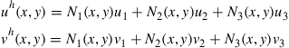
We write the shape functions in the following matrix form:
 (7.9)
(7.9)
where α is the vector of the three unknown constants, and p is the vector of polynomial basis functions (or monomials). Using Eq. (3.21), the moment matrix P corresponding to basis p can be given by
 (7.10)
Note that the above equation is written for the shape functions, and not for the displacements. For this particular problem, we use up to the first order of polynomial basis. Depending upon the problem, we can use a higher order of polynomial basis functions. The complete order of polynomial basis functions in two-dimensional space up to the nth order can be given by using the so-called Pascal triangle, shown in Figure 3.2. The number of terms used in p depends upon the number of nodes the 2D element has. We usually try to use terms of lowest orders to make the basis as complete as possible in order. It is also possible to choose specific terms of higher orders for different types of elements. For our triangular element there are three nodes, and therefore the lowest terms with complete first order are used, as shown in Eq. (7.9). The assumption of Eqs. (7.5)–(7.7) implies that the displacement is assumed to vary linearly in the element. In these equations or Eq. (7.8) there are a total of nine constants to be determined. Our task now is to determine these constants.
If the shape functions constructed possess the delta function property, based on Lemmas 2 and 3 given in Chapter 3, the shape functions constructed will possess the partition of unity and linear field reproduction properties, as long as the moment matrix given in Eq. (7.10) is of full rank. Therefore, we can expect that the complete linear basis functions used in Eq. (7.9) guarantee that the shape functions to be constructed satisfy the sufficient requirements for FEM shape functions. What we need to do now is simply impose the delta function property on the assumed shape functions to determine the unknown coefficients ai, bi, and ci.
The delta functions property states that the shape function must be a unit at its home node, and zero at all the remote nodes. For a two-dimensional problem, it can be expressed as
 (7.11)
For a triangular element, this condition can be expressed explicitly for all three shape functions in the following equations. For shape function N1, we have
 (7.12)
This is because node 1 at (x1, y1) is the home node of N1, and nodes 2 at (x2, y2) and 3 at (x3, y3) are the remote nodes of N1. Using Eqs. (7.5) and (7.12), we have
 (7.13)
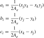
Solving the simultaneous Eq. (7.13) for a1, b1, and c1, we obtain
![]() (7.14)
(7.14)
where Ae is the area of the triangular element that can be calculated using the determinant of the moment matrix:
 (7.15)
Note here that as long as the area of the triangular element is non-zero, or as long as the three nodes are not on the same line, the moment matrix P will be of full rank.
Substituting Eq. (7.14) into Eq. (7.5), we obtain
![]() (7.16)
(7.16)
which can be re-written as
![]() (7.17)
(7.17)
This equation clearly shows that N1 is a plane in the space of (x, y) that passes through the line of 2–3, and vanishes at nodes 2 at (x2, y2) and 3 at (x3, y3). This plane also passes the point of (x1, y1, 1), which guarantees the unity of the shape function at the home node. Since the shape function varies linearly within the element, N1 can then be easily plotted as in Figure 7.5a.

Similarly, making use of these features of N2, we can immediately write out the other two shape functions for nodes 2 and 3. For node 2, the conditions are
 (7.18)
and the shape function N2 should pass through the line 3–1, which gives
 (7.19)
which is plotted in Figure 7.5b. For node 3, the conditions are
 (7.20)
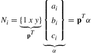
and the shape function N3 should pass through the line 1–2, and is given by
 (7.21)
which is plotted in Figure 7.5c. The process of determining these constants is basically simple, algebraic manipulation.
Finally, the shape functions are summarized in the following concise form:
![]() (7.22)
(7.22)
with
 (7.23)
where the subscript i varies from 1 to 3, and j and k are determined by the cyclic permutation in the order of i, j, k. For example, if i = 1, then j = 2, k = 3. When i = 2, then j = 3, k = 1.
7.2.3 Area coordinates
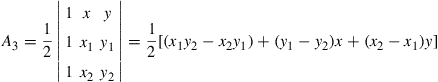
Another alternative and effective method for creating shape functions for triangular elements is to use what is called area coordinates L1, L2, and L3. The use of the area coordinates will immediately lead to the shape functions for triangular elements. However, we first need to define the area coordinates.
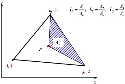
In defining L1, we consider a point P at (x, y) inside the triangular element, as shown in Figure 7.6, and form a sub-triangle of 2–3–P. The area of this sub-triangle is noted as A1, and it can be calculated using the formula
 (7.24)
The area coordinate L1 is then defined as
![]() (7.25)
(7.25)
Similarly, for L2 we form sub-triangle 3–1–P with an area of A2 given by
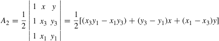 (7.26)
The area coordinate L2 is then defined as
![]() (7.27)
(7.27)
![]() (7.28)
(7.28)
where A3 is the area of the sub-triangle 1–2–P and is calculated using
 (7.29)
It is very easy to confirm the unity property of the area coordinates L1, L2, and L3. First, they are partitions of unity, i.e.,
![]() (7.30)
(7.30)
that can be proven using the definition of the area coordinates:
![]() (7.31)
(7.31)
Secondly, these area coordinates are of delta function properties. For example, L1 will definitely be zero if P is at the remote nodes 2 and 3, and it will be a unit if P is at its home node 1. The same arguments are also valid for L2 and L3.
These two properties are exactly those defined for shape functions. Therefore, we immediately have
![]() (7.32)
(7.32)
The previous equation can also be easily confirmed by comparing Eqs. (7.16) with (7.25), (7.19) with (7.27) and (7.21) with (7.28). The area coordinates are very convenient for constructing higher order shape functions for triangular elements.
Once the shape function matrix has been developed, one can write the displacement at any point in the element in terms of nodal displacements in the form of Eq. (7.1). The next step is to develop the strain matrix so that we can write the strain, and hence the stress, at any point in the element in terms of the nodal displacements. This will further lead to the element matrices.
7.2.4 Strain matrix
Let’s now move to the second step, which is to derive the strain matrix required for computing the stiffness matrix of the element. According to the discussion in Chapter 2, there are only three major stress components, σT = {σxx σyy σxy} in a 2D solid, and the corresponding strains, εT = {εxx εyy γxy} can be expressed as
 (7.33)
or in a concise matrix form,
![]() (7.34)
(7.34)
where L is called a differential operation matrix, and can be obtained simply by inspection of Eq. (7.33):
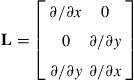 (7.35)
Substituting Eq. (7.1) into Eq. (7.34), we have
![]() (7.36)
(7.36)
where B is termed the strain matrix, which can be obtained by the following equation once the shape function is known:
 (7.37)
Equation (7.36) implies that the strain is now expressed by the nodal displacement of the element using the strain matrix. Equations (7.36) and (7.37) are applicable for all types of 2D elements.
Using Eqs. (7.3), (7.22), (7.23), (7.37), and evaluating the partial derivatives for the shape functions, the strain matrix B for the linear triangular element can be easily obtained, to have the following simple form:
 (7.38)
It can be clearly seen that the strain matrix B for a linear triangular element is a constant matrix. This implies that the strain within a linear triangular element is constant, and thus so is the stress. Therefore, the linear triangular elements are also referred to as constant strain elements or constant stress elements. In reality, stress or strain varies across the structure. Using linear triangular elements with a coarse mesh will therefore result in inaccurate stress or strain distribution. We would need to have a fine mesh of linear triangular elements in order to show an appropriate variation of stress or strain across the structure.
7.2.5 Element matrices
Having obtained the shape function and the strain matrix, the displacement and strain (hence the stress) can all be expressed in terms of the nodal displacements of the element. The element matrices, like the stiffness matrix ke, mass matrix me, and the nodal force vector fe, can then be found using the equations developed in Chapter 3.
The element stiffness matrix ke for 2D solid elements can be obtained using Eq. (3.71):
 (7.39)
Note that the material constant matrix c has been given by Eqs. (2.31) and (2.32) for plane stress and plane strain problems, respectively. Since the strain matrix B is a constant matrix, as shown in Eq. (7.38), and the thickness of the element is assumed to be uniform, the integration in Eq. (7.39) can be carried out very easily, which leads to
![]() (7.40)
(7.40)
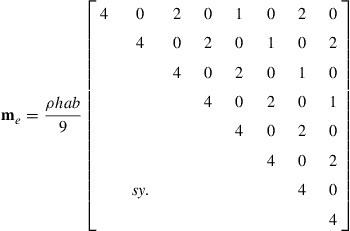
The element mass matrix me can also be easily obtained by substituting the shape function matrix into Eq. (3.75):
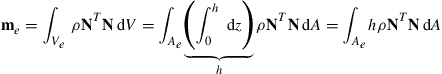 (7.41)
For elements with uniform thickness and density, they can be taken out of the integral and we can rewrite Eq. (7.41) as
 (7.42)
The integration of all the terms in the mass matrix can be carried out simply by using a mathematical formula developed by Eisenberg and Malvern (1973):
![]() (7.43)
(7.43)
where Li = Ni is the area coordinates for triangular elements that is the same as the shape function, as we have seen in Section 7.2.2. The element mass matrix me is found to be
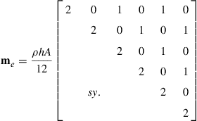 (7.44)
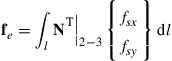
The nodal force vector for 2D solid elements can be obtained using Eqs. (3.78), (3.79), and (3.81). For the case when the element is loaded by a distributed force fs on the edge 2–3 of the element, as shown in Figure 7.4, the nodal force vector involves the surface integral, which in this case is the line integral around the perimeter of the triangular element. Since the external force is zero on all edges except along the edge 2–3, the line integral can be written as
 (7.45)
If the load is uniformly distributed, fsx and fsy are constants within the element, so the above equation becomes
 (7.46)
where l2–3 is the length of the edge 2–3 of the element. The force vector above is obtained by the integral of the linear shape functions, N2 and N3, along the edge 2–3, which can be easily shown to be l2–3/2. Note that for a uniformly distributed load, the equivalent force components acting on the edge 2–3 (fsxl2–3 and fsyl2–3) are shared equally by the two nodes 2 and 3.
Once the element stiffness matrix ke, mass matrix me and nodal force vector fe have been obtained, the global FE equation can be obtained by assembling the element matrices by summing up the contribution from all the adjacent elements at the shared nodes.
7.3 Linear rectangular elements
Triangular elements are usually not preferred by many analysts nowadays, unless there are difficulties with the meshing and re-meshing of models of complex geometry. The main reason is that the triangular elements are usually much less accurate than rectangular or quadrilateral (four-sided) elements. As shown in the previous section, the strain matrix of the linear triangular elements is constant, accounting partially for the inaccuracy. For the rectangular element, the strain matrix is not a constant, as will be shown in this section. This will provide a more realistic presentation in the strain, and hence the stress distribution, across the solid. The formulation of the equations for the rectangular elements is simpler compared to the more general quadrilateral elements, because the shape functions can be formed very easily due to the regularity in the shape of the rectangular element. The simple three-step procedure is applicable, and will be shown in the following sections.
7.3.1 Shape function construction
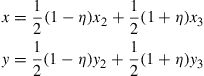
Consider a 2D domain. The domain is discretized into a number of rectangular elements with four nodes and four straight edges, as shown in Figure 7.7. As always, we number the nodes in each element 1, 2, 3, and 4 in a counter-clockwise direction. Note also that, since each node has two DOFs, the total DOFs for a linear rectangular element would be eight. The dimension of the element is defined here as 2a × 2b × h. A dimensionless local natural coordinate system (ξ, η) with its origin located at the center of the rectangular element is defined. The relationship between the physical coordinate (x, y) and the local natural coordinate system (ξ, η) is given by
![]() (7.47)
(7.47)
Equation (7.47) defines a very simple coordinate mapping between physical and natural coordinate systems for rectangular elements as shown in Figure 7.8. Our formulation can now be based on the natural coordinate system. The benefits of the use of natural coordinates include the ease of constructing shape functions and of evaluating matrix integrations over a dimensionless domain. This kind of coordinate mapping technique is one of the most frequently used techniques in the FEM. It is extremely powerful when used for developing elements of complex shapes.
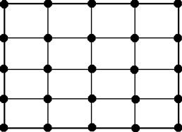

Figure 7.8 Rectangular element and the coordinate systems. (a) Rectangular element in physical system; (b) Square element in natural coordinate system.
We perform the field variable interpolation and express the displacement within the element as an interpolation of the nodal displacements using shape functions. The displacement vector U is assumed to have the form
![]() (7.48)
(7.48)
where the nodal displacement vector de is arranged in the form
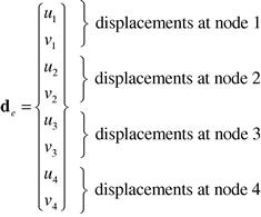 (7.49)
and the matrix of shape functions has the form
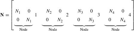 (7.50)
where the shape functions Ni (i = 1, 2, 3, 4) are the shape functions corresponding to the four nodes of the rectangular element.
In determining these shape functions Ni (i = 1, 2, 3, 4), we can follow exactly the same steps used in Sections 4.2.1 or 7.2.2, by starting with an assumption of the displacement or shape functions using polynomial basis functions with unknown coefficients. These unknown coefficients are then determined using the displacements at the nodes of the element or the property of the shape functions. The only difference here is that we need to use four terms of monomials of basis functions. As we have seen in Section 7.2.2, the process can be troublesome and lengthy. In many cases one often uses “shortcuts” to construct shape functions. One of these “shortcuts” is by inspection, and involves utilizing the properties of shape functions.
Due to the regularity of the square element in the natural coordinates, the shape functions in Eq. (7.50) can be written out directly as follows, without going through the detailed process that we described in the previous section for triangular elements:
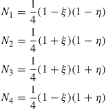 (7.51)
While constructing these shape functions given in Eq. (7.51) by inspection, we make sure that they satisfy the delta function property of Eq. (3.34). For example, for N3 we have
 (7.52)
The same examination of N1, N2, and N4 will confirm the same property.
It is also very easy to show that all the shape functions given in Eq. (7.51) satisfy the partition of unity property of Eq. (3.41):
 (7.53)
The partitions of unity property can also be easily confirmed using Lemma 1 in Chapter 3.
Equation (7.51) should be called a bilinear shape function to be exact, because it varies linearly in both the ξ and η directions, but varies quadratically in any other direction. Denoting the natural coordinates of node j by (ξj, ηj), the bilinear shape function Nj can be re-written in the following concise form:
![]() (7.54)
(7.54)
7.3.2 Strain matrix
Using the same procedure as for the case of the triangular element, the strain matrix B would have the same form as in Eq. (7.37), that is
 (7.55)
It is now clear that the strain matrix for a bilinear rectangular element is no longer a constant matrix since each element in the matrix contains a linear function of either ξ or η. This implies that the strain, and hence the stress, within a bilinear rectangular element is not constant, in contrast to that of the triangular elements given in Eq. (7.38).
7.3.3 Element matrices
Having obtained the shape function and the strain matrix B, the element stiffness matrix ke, mass matrix me, and the nodal force vector fe can be obtained using the equations presented in Chapter 3. Using first the relationship given in Eq. (7.47), we have
![]() (7.56)
(7.56)
Substituting Eq. (7.56) into Eq. (7.39), we obtain
![]() (7.57)
(7.57)
The material constant matrix c has been given by Eqs. (2.31) and (2.32) for plane stress and plane strain problems, respectively. Evaluation of the integral in Eq. (7.57) would not be as straightforward, since the strain matrix B is a function of ξ and η. Even though it is still possible to obtain the closed form for the stiffness matrix by carrying out the integrals in Eq. (7.57) analytically, in practice, we often use a numerical integration scheme to evaluate the integral, and the commonly used Gauss integration scheme will be introduced here. The Gauss integration scheme is a very simple and efficient procedure for numerical integration, and it is briefly outlined here.
7.3.4 Gauss integration
Consider first a one-dimensional integral. Using the Gauss integration scheme, the integral is evaluated simply by a summation of the integrand evaluated at m Gauss points multiplied by corresponding weight coefficients as follows:
 (7.58)
The locations of the Gauss points and the weight coefficients have been found for different m, and are given in Table 7.1. So to perform the integration, all a computer code has to do is to call up the lookup table containing the locations of the Gauss points and the corresponding weight coefficients and perform the summation. In general, the use of more Gauss points will produce more accurate results for the integration. However, excessive use of Gauss points will increase the computational time and use up more computational resources, and it may not necessarily give better results. The appropriate number of Gauss points to be used depends upon the complexity of the integrand.
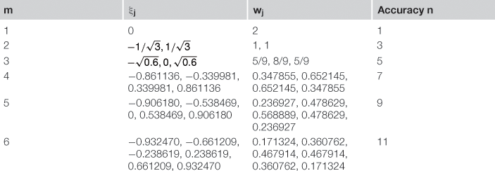
Considering polynomial integrands, it has been proven that the use of m Gauss points gives the exact results of a polynomial integrand of up to an order of n = 2m − 1. For example, if the integrand is a linear function (straight line), we have 2m − 1 = 1, which gives m = 1. This means that for a linear integrand, one Gauss point will be sufficient to give the exact result of the integration. If the integrand is of a polynomial of a third order, we have 2m − 1 = 3, which gives m = 2. This means that for an integrand of a third order polynomial, the use of two Gauss points will be sufficient to give the exact result. The use of more than two points will still give the same results, but takes more computation time. For two-dimensional integrations, the Gauss integration is sampled in two directions, as follows:
 (7.59)
Figure 7.9b shows the locations of four Gauss points used for integration in a square region.

The element stiffness matrix ke can be obtained by numerically carrying out the integrals in Eq. (7.57) using the Gauss integration scheme shown in Eq. (7.59). 2 × 2 Gauss points shown in Figure 7.9b are sufficient to obtain the exact solution for the stiffness matrix given by Eq. (7.57). This is because the entry in the strain matrix, B, is a linear function of ξ or η. The integrand in Eq. (7.57) consists of BTcB, which implies multiplications of two linear functions, and hence this becomes a quadratic function. In Table 7.1, having two Gauss points sampled in each direction is sufficient to obtain the exact results for a polynomial function in that direction of an order up to 3. Figure 7.9a and c show some other different functions and possible number of integration points in a square region.
To obtain the element mass matrix me, we substitute Eq. (7.56) into Eq. (3.75) to obtain
 (7.60)
Upon evaluation of the integral, after substitution of Eq. (7.50) into Eq. (7.60), the element mass matrix me is obtained explicitly as
 (7.61)
To evaluate integrals in the mass matrix, the following has been carried out and repeatedly used:
 (7.62)
where i and j are the usual indices for the nodes. For example, in calculating m33, we use the above equation to obtain
![]() (7.63)
(7.63)
In practice, the integrals in Eq. (7.60) are often calculated numerically using the Gauss integration scheme.
The nodal force vector for a rectangular element can be obtained by using Eqs. (3.78), (3.79), and (3.81). Suppose the element is loaded by a distributed force fs on edge 2–3 of the element, as shown in Figure 7.8; the nodal force vector becomes
 (7.64)
If the load is uniformly distributed within the element edge, and fsx and fsy are constant, the above equation becomes
 (7.65)
where b is the half length of the side 2–3. Equation (7.65) suggests that the evenly distributed load is divided equally onto nodes 2 and 3.
The stiffness matrix ke, mass matrix me, and nodal force vector fe can be used directly to assemble the global FE equation, Eq. (3.96). Coordinate transformation is needed if the orientation of the local natural coordinate does not coincide with that of the global coordinate system. In such a case, quadrilateral elements are often used, which will be developed in the next section.
7.4 Linear quadrilateral elements
Though the rectangular element can be very useful, and is usually much more accurate than the triangular element, it is difficult to use for problems with any geometry other than rectangles. Hence, its practical application is very limited. A much more practical and useful element would be the general quadrilateral element, that can have unparalleled edges. However, there can be a problem for the integration of the mass and stiffness matrices for a quadrilateral element, because of the irregular shape of the integration domain. The Gauss integration scheme cannot be implemented directly with quadrilateral elements. Therefore, what is required first is to map the quadrilateral element into the natural coordinates system to become a square element, so that the shape functions and the integration method used for the rectangular element can be utilized. Hence, the key in the development of a quadrilateral element is the coordinate mapping. Once the mapping is established, the rest of the procedure is exactly the same as that used for formulating the rectangular element in the previous section.
7.4.1 Coordinate mapping
Figure 7.10 shows a 2D domain with the shape of an airplane wing. As you can imagine, dividing such a domain into rectangular elements of parallel edges is impossible. The job can be easily accomplished by the use of quadrilateral elements with four straight but unparallel edges, as shown in Figure 7.10. In developing the quadrilateral elements, we use the same idea of coordinate mapping that was used for the rectangular elements in the previous section. Due to the deviation from regularity of the element shape, the mapping will become a little more involved, but the procedure is basically the same. In fact, the mapping carried out for the rectangular element is just a specific case of the more general procedure that will be described for the quadrilateral element.
Consider now a quadrilateral element with four nodes numbered 1, 2, 3, and 4 in a counter-clockwise direction, as shown in Figure 7.11. The coordinates for the four nodes are indicated in Figure 7.11a in the physical coordinate system. The physical coordinate system can be the same as the global coordinate system for the entire structure. As there are two DOFs at a node, a linear quadrilateral element has a total of eight DOFs, like the rectangular element. A local natural coordinate system (ξ, η), as shown in Figure 7.11b, with its origin at the center of the squared element mapped from the global coordinate system is used to construct the shape functions, and the displacement is interpolated using the equation
![]() (7.66)
(7.66)

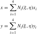
Equation (7.66) represents a field variable interpolation using the nodal displacements. Using a similar concept, we can also interpolate the coordinates x and y themselves. In other words, we let coordinates x and y be interpolated from the nodal coordinates using the shape functions which are expressed as functions of the natural coordinates. This coordinate interpolation is mathematically expressed as
![]() (7.67)
(7.67)
where X is the vector of the physical coordinates,
 (7.68)
and N is the matrix of shape functions given by Eq. (7.50). In Eq. (7.67), xe represents the physical coordinates at the nodes of the element, given by
 (7.69)
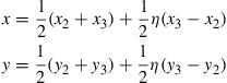
Equation (7.67) can also be expressed explicitly as
 (7.70)
where Ni is the shape function defined for the rectangular element in Eqs. (7.53), or (7.54). Each of the physical coordinates (x and y) is now a function of the natural coordinates, ξ and η. Note that, due to the unique property of the shape functions, the interpolation at these nodes will be exact. For example, substituting ξ = 1 and η = −1 in Eq. (7.70) gives x = x2 and y = y2, as shown in Figure 7.11. Physically, this means that point 2 in the natural coordinate system is mapped to point 2 in the physical coordinate system, and vice versa. The same can also be easily observed for points 1, 3, and 4. The coordinate mapping that was carried out for the rectangular element is a specific case of this more general mapping using the shape functions. For the case of the rectangular element, the regularity results in only a scaling of the x and y axes such that x is a function of only ξ and y is a function of only η.
Let’s now analyze this mapping more closely. Substituting ξ = 1 into Eq. (7.70) gives
 (7.71)
or
 (7.72)
Eliminating η from the above two equations gives
![]() (7.73)
(7.73)
which represents a straight line connecting the points (x2, y2) and (x3, y3). This means that edge 2–3 in the physical coordinate system is mapped onto edge 2–3 in the natural coordinate system. The same can be observed for the other three edges. Hence, we can see that the four straight edges of the quadrilateral in the physical coordinate system correspond to the four straight edges of the square in the natural coordinate system. Therefore, the full domain of the quadrilateral element is mapped onto a squared natural coordinate system.
7.4.2 Strain matrix
After mapping is performed for the coordinates, we can evaluate the strain matrix B. To do so in this case, it is necessary to express the differentials in terms of the natural coordinates, since the relationship between the x and y coordinates and the natural coordinates is no longer a trivial case of scaling in the ξ and η, respectively, as in the case for rectangular elements. Utilizing the chain rule in application to partial differentiation, we have
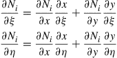 (7.74)
The above equations can be written in the matrix form
 (7.75)
where J is the Jacobian matrix defined by
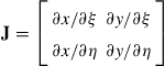 (7.76)
We now substitute the interpolation of the coordinates defined by Eq. (7.70) into the above equation, and obtain
 (7.77)
Rewriting Eq. (7.75) to obtain
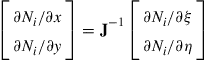 (7.78)
which gives the relationship between the differentials of the shape functions with respect to x and y with those with respect to ξ and η. We can now use the equation B = LN to compute the strain matrix B, by replacing all the differentials of the shape functions with respect to x and y with those with respect to ξ and η, obtained using Eq. (7.78). This process can be easily implemented by a computer code.
7.4.3 Element matrices
Once the strain matrix B has been obtained, we can proceed to evaluate the element matrices. The stiffness matrix can be obtained by Eq. (7.39). To evaluate the integration, the following formula, which has been proven by Murnaghan (1951), can be used:
![]() (7.79)
(7.79)
where det |J| is the determinate of the Jacobian matrix. Hence, the element stiffness matrix can be written as
![]() (7.80)
(7.80)
The above integrals can then be evaluated using the Gauss integration scheme discussed in the previous section. Notice how the coordinate mapping enables us to use the Gauss integration scheme over a simple squared area.
The shape function defined by Eq. (7.53) is a bilinear function of ξ and η. The elements in the strain matrix B are obtained by differentiating these bilinear functions with respect to ξ and η, and by multiplying the inverse of the Jacobian matrix whose elements are also bilinear functions. Therefore, the elements of BTcBdet|J| are quite complicated and may not be expressed by polynomials. This means that such a stiffness matrix may not, in general, be evaluated exactly using the Gauss integration scheme, unlike the case for the rectangular element.
The element mass matrix me can also be evaluated in the same way as for the rectangular element using Eq. (7.60):
 (7.81)
The element force vector is obtained in the same way as described for the rectangular element. For a distributed load acting on one of the edges, the integral only involves one-dimensional line integrals like before and there is thus no change in the way the integration is carried out. Having obtained the element matrices, the usual method of assembling the element matrices is carried out to obtain the global matrices.
7.4.4 Remarks
The shape functions used to interpolate the coordinates in Eq. (7.70) are the same as those used for interpolation of the displacements. Such an element is called an isoparametric element. However, the shape functions for coordinate and displacement interpolations do not necessarily have to be the same. Using different shape functions for coordinate and displacement interpolations will lead to the development of what is known as subparametric or superparametric elements. These elements have been studied in academic research, but are less often used in practical applications. Details of such elements will not be covered in this book.
7.5 Elements for axisymmetric structures
In engineering applications, there are structures made by revolving a plane of arbitrary shape with respect to an axis, forming so-called axisymmetric structures, as shown in Figure 7.12. Such axisymmetric structures can often be modeled as 2D plane problems. In such cases, we formulate the problem in the cylindrical coordinate system of r, z, and θ, where r is the radial direction from the axis of rotation, z is the direction along the axis of rotation, and θ is the circumferential direction (following counter-clockwise convention). If the geometry, boundary conditions, loadings, and material properties of the geometry are independent of the circumferential direction, θ, the problem is essentially a 2D one. We can then reduce the problem domain drastically to a 2D “cross-section” in the r–z plane or θ = constant plane as shown schematically in Figure 7.12.

Figure 7.12 Reduction of a 3D axisymmetric problem into a 2D planar problem using axisymmetric elements.
In order to formulate 2D axisymmetric elements, we shall define the displacement field by two components in the r–z plane: u for displacement in the r or radial direction; and w for displacement in the z or axial direction. Because of the axisymmetric behavior, the asymmetric strain components shall vanish, and we have
![]() (7.82)
(7.82)
Note that the so-called hoop strain, ![]() , is not zero in general. The strain components are defined as:
, is not zero in general. The strain components are defined as:
 (7.83)
Expressing this in a matrix form, we obtain
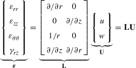 (7.84)
where L is the differential operator matrix for 2D axisymmetric problems. Equation (7.84) shows that the strain definition is similar to plane stress or plane strain problems described earlier in this chapter except for the additional hoop strain, εθθ, that does not change with θ. As a result, the third row in the differential operator matrix, L, does not contain a differential operator but a multiplier with the radial displacement, u. Because of this extra hoop strain, a uniform displacement in the radial displacement, without additional boundary conditions in the radial direction, no longer produces a rigid body motion, but instead produces a circumferential strain. Correspondingly, the stress components associated with the 2D axisymmetric element are σrr, σzz, σθθ, and σrz, where σθθ is the hoop stress. If we approximate the displacement field by U = Nde, like before, Eq. (7.84) can then be written as
![]() (7.85)
(7.85)
where B = LN and the shape functions Ni in N will depend on the type of element (triangular, rectangular or quadrilateral) as described in earlier sections of this chapter.
The matrix of elastic constants, c, for the 2D axisymmetric problem, can be obtained from that of a 3D solid by imposing the conditions of γrθ = γzθ = 0 and by assuming that the shear strain, γrz, is not coupled with the hoop stress, σθθ. For a 2D, axisymmetric isotropic material, the matrix of elastic constants is given as
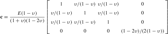 (7.86)
The element matrices can then be obtained in a similar way as for a 2D element, but with special care on the integration. By considering the small volume element, dV, as small volumetric “rings,” it becomes
![]() (7.87)
(7.87)
and the element stiffness matrix can be obtained using Eq. (3.71) as
![]() (7.88)
(7.88)
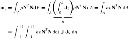
Similarly, the element mass matrix can be obtained from Eq. (3.75) as
![]() (7.89)
(7.89)
The element force vector can be obtained from Eqs. (3.78), (3.79)), and (3.81) with the necessary substitution of Eq. (7.87) for the body force term (Eq. (3.78)). For the surface force term, Eq. (3.79), dS becomes
![]() (7.90)
(7.90)
and, therefore, the element force vector can be expressed as
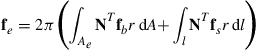 (7.91)
where fb is the vector of body force per unit volume and fs is the vector of traction force per unit area. With the element matrices obtained, the remaining procedures of assembling the element matrices into the global matrix equation, prescription of boundary conditions and loads, and solving the system of linear equations follow.It should also be noted that the plane strain element is an extreme case of the axisymmetric element when r becomes very large. In this case, the contribution of the hoop strain, ![]() , is negligible and, therefore, the third row and third column of Eq. (7.86) can be ignored and the c matrix becomes that for the case of plane strain problems.
, is negligible and, therefore, the third row and third column of Eq. (7.86) can be ignored and the c matrix becomes that for the case of plane strain problems.
7.6 Higher order elements—triangular element family
7.6.1 General formulation of shape functions
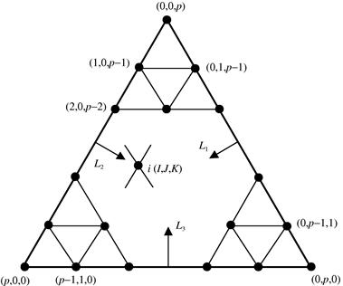
In developing higher order elements, we make use of the area coordinate system. Figure 7.13 shows a general triangular element of order p that has nd nodes calculated by
![]() (7.92)
(7.92)
Node i (I, J, K) is located at the Ith node in the L1 direction, at the Jth node in the L2 direction, and at the Kth node in the L3 direction. I, J, and K are indexed from zero as illustrated in Figure 7.13. From Figure 7.13, we have at any node that
![]() (7.93)
(7.93)
The shape function can be written in the form (Argyris et al., 1968)
![]() (7.94)
(7.94)
where ![]() , and
, and ![]() are defined by Eq. (4.73), but the coordinate ξ is replaced by the area coordinates, i.e.,
are defined by Eq. (4.73), but the coordinate ξ is replaced by the area coordinates, i.e.,
![]() (7.95)
(7.95)
where α = 1, 2, 3; β = I, J, K. For example, when α = 1 and β = I, we have
![]() (7.96)
(7.96)
 (7.97)
it is easy to verify that the delta function property is satisfied, i.e.,
 (7.98)
From Eqs. (7.94) and (7.95), the order of the shape function can be found to be the same as
![]() (7.99)
(7.99)
Since Lα is a linear function of x and y, the order of the shape function will be
![]() (7.100)
(7.100)
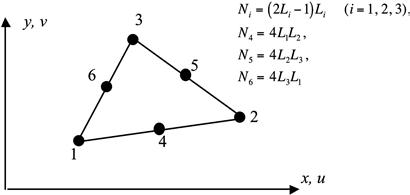
7.6.2 Quadratic triangular elements
Consider a quadratic triangular element as shown in Figure 7.14. The element has six nodes: three corner nodes and three mid-side nodes. Using Eqs (7.94) and (7.95), the shape functions can be obtained very easily. Here we demonstrate the calculation of N1. Note that for the element shown in Figure 7.14, the area coordinate L1 has three coordinate values:
 (7.101)
Using Eq. (7.94), we have
 (7.102)
For the other two corner nodes, 2, 3, we should have exactly the same equation:
![]() (7.103)
(7.103)
For the mid-side node 4, we have
 (7.104)
This equation is also valid for the other two mid-nodes, and therefore we have
![]() (7.105)
(7.105)
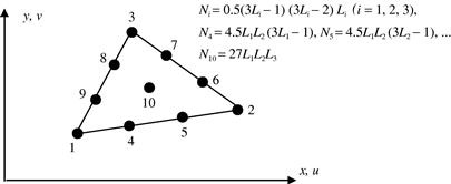
7.6.3 Cubic triangular elements
For the cubic triangular element shown in Figure 7.15 that has nine nodes, the shape function can also be obtained using Eq. (7.94), as well as four area coordinate values of (taking L1 as an example)
 (7.106)
We omit the details of the evaluation process and list the results below. The reader is encouraged to confirm the results. For corner nodes (1, 2, and 3):
![]() (7.107)
(7.107)
For side nodes (4–9):
![]() (7.108)
(7.108)
For the interior node (10):
![]() (7.109)
(7.109)
7.7 Rectangular Elements
7.7.1 Lagrange type elements
Considering a rectangular element with nd = (n + 1)(m + 1) nodes, shown in Figure 7.16. The element is defined in the domain of (−1 ≤ ξ ≤ 1, −1 ≤ η ≤ 1) in the natural coordinates ξ and η. Due to the regularity of the nodal distribution along both the ξ and η directions, the shape function of the element can be simply obtained by multiplying one-dimensional shape functions with respect to the ξ and η directions using the Lagrange interpolants defined in Eq. (4.73) (Zienkiewicz and Taylor, 2000):
![]() (7.110)
(7.110)
Due to the delta function property of the 1D shape functions given in Eq. (4.74), it is easy to confirm that the Ni given by Eq. (7.110) also has the delta function property.

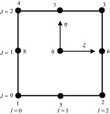
Using Eqs. (7.110) and (4.73), the nine-node quadratic element shown in Figure 7.17 can be given by
 (7.111)
From Eq. (7.111), it can easily be seen that all the shape functions are formed using the same set of nine basis functions:
![]() (7.112)
(7.112)
which are linearly-independent. From Lemma 2 in Chapter 3, we can expect that the shape functions given in Eq. (7.111) to be partitions of unity. In addition, because the basis functions also contain the linear basis functions, these shape functions can also be expected to have linear field reproduction (Lemma 3), at least. Hence, they satisfy the sufficient requirements for FEM shape functions. Any other high order Lagrange type of rectangular element can be created in exactly the same way as for the nine-node element.
7.7.2 Serendipity type elements
The method used in constructing the Lagrange type elements is very systematic. However, the Lagrange type of elements is not very widely used, due to the presence of the interior nodes. Serendipity type elements are created by inspective construction methods. For these elements, we intentionally construct high order elements without interior nodes.
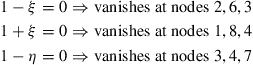
Consider the eight-node element shown in Figure 7.18a. The element has four corner nodes and four mid-side nodes. The shape functions in the natural coordinates for the quadratic rectangular element are given as
 (7.113)
where (ξj, ηj) are the natural coordinates of node j. It is very easy to observe that the shape functions possess the delta function property. The shape function is constructed by simple inspections making use of the shape function properties. For example, for the corner node 1 (where ξ1 = −1, η1 = −1), the shape function N1 has to pass the following three lines as shown in Figure 7.19 to ensure its vanishing at remote nodes:
 (7.114)
The shape N1 can then immediately be written as
![]() (7.115)
(7.115)
where C is a constant to be determined using the condition that it has to be unity at node 1 at (ξ1 = −1, η1 = −1), which gives
![]() (7.116)
(7.116)
We finally have
![]() (7.117)
(7.117)
which is the first equation in Eq. (7.113) for j = 1.


Figure 7.19 Construction of the 8-node element serendipity element. Three straight lines passing through the remote nodes of node 1 are used.
Shape functions at all the other corner nodes can be constructed in exactly the same manner. As for the mid-side nodes, say node 5, we enforce the shape function to pass through the following three lines as shown in Figure 7.20:
 (7.118)
The shape N5 can then immediately be written as
![]() (7.119)
(7.119)
where C is a constant to be determined using the condition that it has to be unity at node 5 at (ξ5 = 0, η5 = −1), which gives
![]() (7.120)
(7.120)
We finally have
![]() (7.121)
(7.121)
which is the second equation in Eq. (7.113) for j = 5.

Figure 7.20 Construction of the 8-node element serendipity element. Three straight lines passing through the remote nodes of node 5 are used.
Because the delta functions property is used for the shape functions given in Eq. (7.113), they will of course possess the delta function property. It can be easily seen that all the shape functions can be formed using the same set of basis functions
![]() (7.122)
(7.122)
that are linearly-independent. From Lemmas 2 and 3, we confirm that the shape functions are partitions of unity, and at least linear field reproductions. Hence, they satisfy the sufficient requirements for FEM shape functions.
Following a similar procedure, the shape functions for the 12-node cubic element shown in Figure 7.18b can be written as
 (7.123)
The reader is encouraged to figure out what lines or curves should be used to form the shape functions listed in Eq. (7.123). When η = ηi = 1, the above equations reduce to the one-dimensional cases of quadratic and cubic elements defined by Eqs. (4.75) and (4.76), respectively.
7.8 Elements with curved edges
Using high order elements, elements with curved edges can be used in the modeling. Two frequently used higher order elements of curved edges are shown in Figure 7.21a. In formulating these types of elements, the same mapping technique used for the linear quadrilateral elements (Section 7.4) can be used. In the physical coordinate system, elements with curved edges, as shown in Figure 7.21a, are first formed in the problem domain. These elements are then mapped into the natural coordinate system using Eq. (7.67). The elements mapped in the natural coordinate system will have straight edges, as shown in Figure 7.21b.
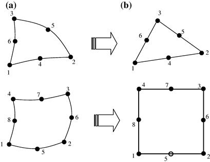
Figure 7.21 2D solid elements with curved edges. (a) Curved elements in the physical coordinate system; (b) Elements with straight edges obtained by mapping.
Higher order elements of curved edges are often used for modeling curved boundaries. Note that elements with excessively curved edges may cause problems in the numerical integration. Therefore, a finer mesh should be used where the curvature of the geometry is large. In addition, it is recommended that in the internal portion of the domain, elements with straight edges should be used whenever possible. More details on modeling issues will be discussed in detail in Chapter 11.
7.9 Comments on Gauss integration
When the Gauss integration scheme is used, one has to decide how many Gauss points should be used. Theoretically, for a one-dimensional integral, using m points can give the exact solution for the integral of a polynomial integrand of up to an order of (2m − 1). As a general rule of thumb, more points should be used for a higher order of elements. It is also noted that using a smaller number of Gauss points tends to counteract the over-stiff behavior associated with the displacement-based FEM.
This over-stiff behavior of the displacement-based FEM comes about primarily because of the use of the shape function. As discussed, the displacement in an element is assumed using shape functions interpolated from the nodal displacements. This implies that the deformation of the element is actually prescribed in the fashion of the shape function. This gives a constraint to the element, and thus the element behaves more stiffly than it should. It is often observed that higher order elements are usually softer than lower order ones. This is because the use of more nodes decreases the constraint on the element.
Coming back to the Gauss integration issue, two Gauss points for bilinear elements, and about two or three Gauss points in each direction for quadratic elements, should be sufficient for most cases. Many of the explicit FEM codes based on explicit formulation tend to use one-point integration for bilinear elements to achieve the best performance in saving central processing unit (CPU) time.
7.10 Case study: Side drive micro-motor
In this case study, we analyze another microelectromechanical systems (MEMs) device: A common micro-actuator in the form of a side drive electrostatic micro-motor, as shown in Figure 7.22. Such micro-motors are usually made from polysilicon using lithographic techniques. Their diameters vary depending on the design, with the first designs having diameters of 60–120 μm. Of course, the actual working dynamics of the micro-motor will be rather complex to model, though it can still be readily done if required. Therefore, to illustrate certain points pertaining to the use of basic 2D solid elements, we use the geometrical and material information for this micro-motor and apply arbitrary loading and boundary conditions to it.

Isotropic material properties will be employed here to makes things less complicated. The material properties of polysilicon are shown in Table 7.2. We shall do a stress analysis on the rotor with some loading condition on the rotor blades. Examining the geometry, loading, and boundary conditions of the rotor in Figure 7.22, we can see that it is symmetrical, i.e., we need not model the full rotor, but rather we can just model say one quarter of the rotor and apply the necessary boundary conditions. We can do this since this one-quarter model will be repeated geometrically anyway. Of course, we can even model one eighth of the model and the results will be the same if the condition of repetitive symmetry is properly applied. Hence, this becomes a neat and efficient way of modeling repetitive or symmetrical geometry.
Table 7.2
Elastic properties of polysilicon.
| Young’s Modulus, E | 169 GPa |
| Poisson’s ratio, ν | 0.262 |
| Density, ρ | 2300 kg m−3 |
7.10.1 Modeling
Figure 7.23 shows one-quarter of the full model of the micro-motor rotor. We take the diameter of the whole rotor to be 100 μm and the depth or thickness to be 13 μm, to correspond with realistic values of micro-motor designs. The geometry can be easily drawn using pre-processors like PATRAN, ABAQUS CAE or using basic CAD software, after which it can be imported into appropriate pre-processors for meshing. Note that pre-processors are software packages used to aid us in visualizing the geometry, and to mesh up the geometry using finite elements, especially for complicated geometries. To illustrate the formulation of the FE equations clearly, we would initially mesh up the geometry in Figure 7.23 with a coarse mesh, as shown in Figure 7.24. Four-nodal, quadrilateral elements are used with a total of 24 elements and 41 nodes in the model. We shall increase the number of elements (and nodes) in later analyses to compare the results. Since the depth or thickness of the motor is much smaller than the other dimensions, and the external forces are assumed to be within the plane of the rotor, we can assume plane stress conditions.


In the above figure, it can also be seen that a distributed force of 10 N/m is applied compressively to the rotor blades. The center hole in the rotor, which is supposed to be the location for a “hub” to keep the rotor in place, is assumed to be constrained. The nodes along the edge y = 0 are constrained in the y direction and the nodes along the edge x = 0 are constrained in the x direction. These are to simulate the symmetrical boundary conditions of the model, since those nodes are not supposed to move in the direction normal to the plane of symmetry.
7.10.2 ABAQUS input file
The ABAQUS input file for the above described FE model is shown below. Note that some parts of the input file containing the data values are left out to limit the length of the file in this book. The text boxes to the right of the input file are not part of the file, but rather explain what the sections of the file mean.


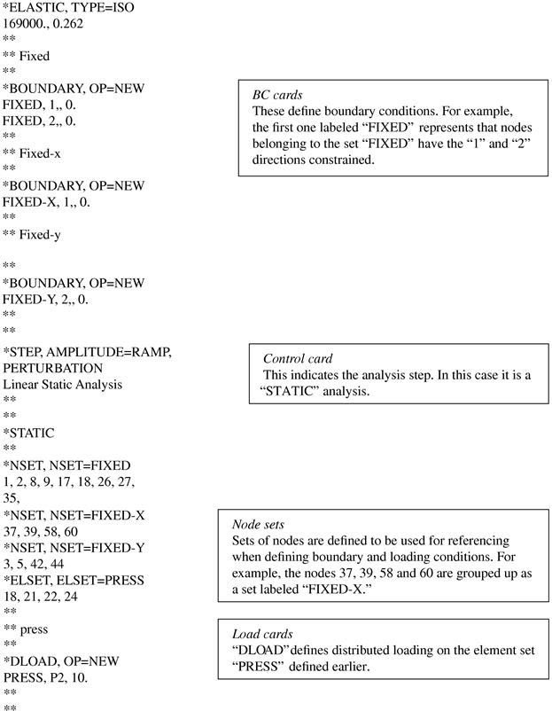
The input file above shows how a basic ABAQUS input file can be set up. It should be noted that the units used in this case study are micrometers, and all the conversions of the necessary inputs is done for consistency, as before.
7.10.3 Solution process
Let’s now try to relate the information we provided in the input file with what is covered in this chapter. As before, the first sets of data usually defined are the nodes and their coordinates. Then, there are the element cards containing the connectivity information. The importance of this information has already been mentioned in previous case studies. Looking at Figure 7.24, it is not difficult to guess that the element used is an isoparametric quadrilateral element (CPS4–2D, quadrilateral, bilinear, plane stress elements), rather than that of a rectangular element. Obviously, it can be visualized that using rectangular elements would pose a problem in meshing the geometry here. In fact, the use of purely rectangular elements is so rare that most software (including ABAQUS) only provides the more versatile quadrilateral element. This information from the nodal and element cards will be used for constructing the element matrices (see, Eqs. (7.80) and (7.81)).
Next, the property cards define the properties of the elements, and also specify the material the elements should possess. For the plane stress elements, the thickness of the elements must be specified (13 μm in this case), since it is required in the stiffness and mass matrices (the mass matrix is actually not required in this case study, since this is a static analysis). Similarly, the elastic properties of the polysilicon material defined in the material card are also required in the element matrices. It should be noted that in ABAQUS, the integral in Eq. (7.80) is evaluated using the Gauss integration scheme, and the default number of Gauss points for the bilinear element is 4.
The boundary (BC) cards define the boundary conditions for the model. To model the symmetrical boundary conditions, at the lines of symmetry (x = 0 and y = 0), the nodal displacement component normal to the line is constrained to zero. The nodes (node set, FIXED) along the center hole where the hub should be is also fully clamped in. The load cards defined specify the distributed loading on the motor, as shown in Figure 7.24. These will be used to form the force vector, which is similar in form to that of Eq. (7.64).
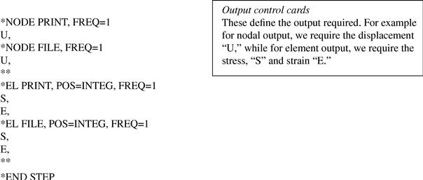
The control cards are used to control the analysis, which in this case defines that this is a static analysis. Finally, the output cards define the necessary output requested, which here are the displacement components, the stress components, and the strain components.
Once the input file has been created, one can then invoke ABAQUS to execute the analysis, and the results will be written into an output file that can be read by the post-processor.
7.10.4 Results and discussion
Using the above ABAQUS input file that describes the problem, a static analysis is carried out. Figure 7.25 shows the Von Mises stress distribution obtained with 24 bilinear quadrilateral elements. It should be noted here that 24 elements (41 nodes) for such a problem may not be sufficient for accurate results. Analyses with a denser mesh (129 nodes and 185 nodes) using the same element type are also carried out. Their input files will be similar to that shown, but with more nodes and elements.

Figure 7.26 and Figure 7.27 show the Von Mises stress distribution obtained using 96 (129 nodes) and 144 elements (185 nodes), respectively. Figure 7.28 also shows the results obtained when 24 eight-nodal elements (105 nodes in total) are used instead of four-nodal elements. The element type in ABAQUS for an eight-nodal, plane stress, quadratic element is “CPS8.” Finally, linear, triangular elements (CPS3) are also used for comparison, and the stress distribution obtained is shown in Figure 7.29.

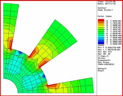
Figure 7.27 Analysis no. 3: Von Mises stress distribution using 144 bilinear quadrilateral elements.
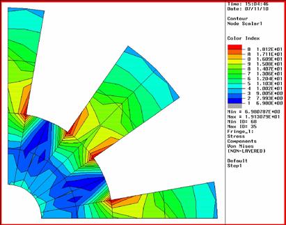
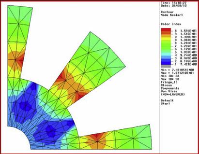
Figure 7.29 Analysis no. 5: Von Mises stress distribution using 192 three-nodal, triangular elements.
From the results obtained, it can be noted that analysis 1, which uses 24 bilinear elements, does not seem as accurate as the other three. Table 7.3 shows the maximum Von Mises stress for the five analyses. It can be seen that the maximum Von Mises stress using just 24 bilinear, quadrilateral elements (41 nodes) is just about 0.0139 GPa, which is a bit low when compared with the other analyses. The other analyses, especially from analyses 2 to 4 using quadrilateral elements, obtained results that are quite close to one another when we compare the maximum Von Mises stress. We can conclude that using just 24 bilinear, quadrilateral elements is definitely not sufficient in this case. The comparison also shows that using quadratic elements (eight-nodal) with a total of 105 nodes, yielded results that are close to analysis 3 with the bilinear elements and 185 nodes. In this case, the quadratic elements also have curved edges, instead of straight edges, and this would better define the curved geometry. Looking at the maximum Von Mises stress obtained using triangular elements in analysis 5, we can see that, despite having the same number of nodes as in analysis 2, the results obtained showed some deviation. This clearly shows that quadrilateral elements in general provide better accuracy than triangular elements. However, it is still convenient to use triangular elements to mesh complex geometry containing sharp corners.

From the stress distribution, it can generally be seen that there is stress concentration at the corners of the rotor structure, as expected. Therefore, if structural failure is to occur, it would be at these areas of stress concentration.
7.11 Review questions
1. Figure 7.30 shows a wall that is very thin in the z direction (out of paper), and can be modeled as a 2D problem. It is subjected to a uniform pressure in the x direction on the left edge. Use FEM to perform stress analysis for this problem.
a. Is the problem a plane strain or plane stress problem? Justify your answer.
b. In FEA procedure, what is the difference in modeling a plane strain and a plane stress problem?
c. Explain your strategy to model this particular problem.
d. Sketch a mesh for this problem domain of your model using about 50 elements. (You are not required to consider the stress concentration at the corners.)
e. Provide all the boundary conditions at relevant nodes that are needed to solve this problem using your FEM model.
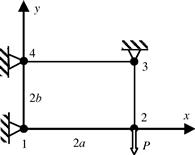
2. Figure 7.31 shows a mesh with 15 equal square elements of width 2a and 24 nodes for a 2D domain. A uniform pressure is applied on edges 1–2–3, and a concentrate load is applied at the middle of edge 3–4. In the input file of the FEM model, there are the following lines defining the connectivity for elements ![]() ,
, ![]() ,
, ![]() ,
, ![]() , and
, and ![]() .
.
5, 12, 11, 5, 6
6, 7, 8, 13, 14
7, 8, 9, 14, 15
8, 15, 16, 10, 9
9, 10, 16, 11, 17
a. Indicate the lines that wrongly define (unconventional) the connectivity of the element. Correct these lines and justify your answer.
b. Give the external force vector. Propose a better way to re-number the nodes and justify your answer.

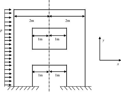
3. Figure 7.32 shows a square 2D solid that is modeled using uniformly distributed square elements. The solid is subjected to a vertical concentrated force P at the top-left corner, a distributed force f = px over part of the top surface, and a uniformly distributed force q on the left edge.

a. Using bilinear square elements for the entire solid, derive the external nodal force vector for nodes 1, 2, 3, 4, 5, and 6.
b. If 8-node quadratic square elements are used instead of the bilinear elements, how is the external nodal force vector computed? You are required only to provide the formulae and explain the procedure.
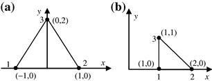
4. Figure 7.33 shows two right-angle triangular elements of base b and height h. Derive the shape functions and the strain matrix B for these two elements.

5. Figure 7.34 shows two right-angle triangular elements of base b and height h. Derive the shape functions and the strain matrix B for these two elements.

6. Consider a plane strain element as shown in Figure 7.35.
a. Calculate the shape functions for the element.
b. The nodal displacements are given as
![]()
c. Calculate the stress components ![]() and the principle stresses σ1 and σ2 for the element, with Young’s modulus E = 70 GPa and Poisson ratio ν = 0.3.
and the principle stresses σ1 and σ2 for the element, with Young’s modulus E = 70 GPa and Poisson ratio ν = 0.3.
d. Determine the principal stresses σ1 and σ2 and the principal angles ![]() , using the following equations:
, using the following equations:
![]()
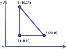
7. Figure 7.36 shows two triangular elements, and the unit for the coordinates is in cm. Let E = 2.1 × 10¹¹ Pa, v = 0.25, and thickness t = 5 mm. Assume plane stress conditions.
a. Calculate shape functions for these triangular elements;
b. Calculate the strain matrix for these triangular elements;
c. Calculate the stiffness matrix for these triangular elements;
d. Determine the stresses ![]() in the element for given nodal displacements (in m) of
in the element for given nodal displacements (in m) of
![]()
e. Determine the principal stresses σ1 and σ2 and the principal angles ![]() , using the Equation given in the previous question.
, using the Equation given in the previous question.
8. Show that the stiffness matrix of an isotropic linear triangular element whose thickness varies linearly in the element is
![]()
where B is the strain matrix, c is the matrix of material constants, Ae is the area of the triangle, and ![]() is the average thickness (h1 + h2 + h3)/3, where h1, h2, and h3 are the nodal thickness at the node.
is the average thickness (h1 + h2 + h3)/3, where h1, h2, and h3 are the nodal thickness at the node.
9. Show that the mass matrix of a linear triangular element whose thickness varies linearly within the plane of the element is

where ρ is the density, Ae is the area, ![]() is the mean thickness, and
is the mean thickness, and ![]() with i = 1, 2, 3 for the three nodes.
with i = 1, 2, 3 for the three nodes.
10. The thickness variation of a linear rectangular element is given by

where Ni is the bilinear shape function, and hi is the thickness value at node i. How many Gauss points are required to evaluate exactly the mass and stiffness matrices.
11. If the thickness variation of a linear quadrilateral is the same as the rectangular element in Problem (3), how many Gauss points are required to evaluate the mass matrix exactly? How many Gauss points are required to integrate the volume of the element exactly? How many Gauss points are required to integrate the stiffness matrix exactly?
12. Construct the shape functions for the 12-node rectangular element for one corner node and one side node.
13. Figure 7.37 shows a plane strain problem to be solved using only two triangular elements.
a. Determine the nodal displacements; (Hint: use results from Question 4 for matrix B).
b. Derive expressions for displacements and the element stresses.

14. Figure 7.38 shows a plane strain problem to be solved using only two triangular elements.
a. Determine the nodal displacements; (Hint: use results from Question 4 for matrix B).
b. Derive the expressions for the displacements and element stresses.
c. Calculate the averaged element stresses.

Figure 7.38 A rectangular 2D solid meshed by two triangular elements subjected to a vertical force at node 2.
15. Figure 7.39 shows a plane strain problem to be solved using only one rectangular element. Determine the nodal displacements and element stresses.
References
1. Argyris JH, Fried I, Scharpf DW. The TET 20 and TEA 8 elements for the matrix displacement method. Aeronautical Journal. 1968;72:618–625.
2. Eisenberg MA, Malvern LE. On finite element integration in natural coordinates. International Journal for Numerical Methods in Engineering. 1973;7:574–575.
3. Murnaghan FD. Finite Deformation of an Elastic Solid. John Wiley & Sons 1951.
4. Zienkiewicz OC, Taylor RL. The Finite Element Method. fifth ed. Butterworth-Heinemann 2000.