
Chapter 6 – Physical Design
“A good head and a good heart are always a formidable combination.”
The Four Stages of Modeling for Teradata
Four core stages are identified as being relevant to any database design task. They are:
1. Requirement Analysis involves figuring out what information the users need and their processing requirements. The output of this is the Business Information Model (BIM) which shows major entities and their relationships. This is sometimes referred to as the Business Model or the Business Impact Model.
2. Logical Modeling determines defining the tables and their relationships, and this should be independent of a particular database or indexing strategy. Teradata works well with a Third Normal Form (3NF) model, and the output defines all tables and their columns and the Primary Key Foreign Key relationships between tables plus all constraints.
3. Activity Modeling involves working with the users to determine the volume, usage, frequency, and integrity analysis of a database. This process also consists of placing any constraints on domains and entities. This is called the Extended Logical Data Model (ELDM).
4. Physical Modeling Using the Activity Model and transforming the logical model into a definition of the physical model that will accelerate queries with the best Primary and Secondary Indexes that best suits a specific hardware and software configuration.
This module will concentrate a great deal on the Physical Modeling.
The Logical Model
This simple logical model shows the Primary Key and Foreign Key relationships between tables.
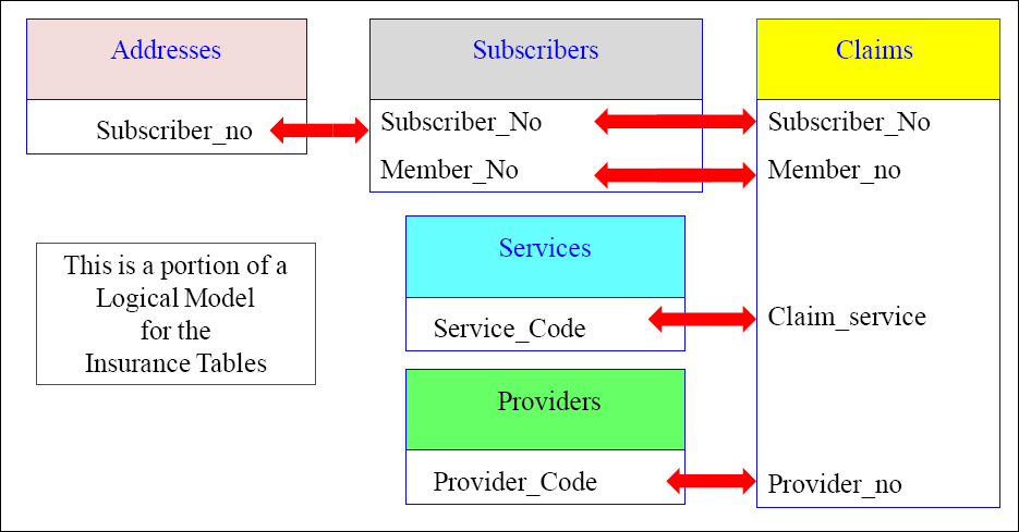
There are five tables above that have a relationship. That means they can be joined together with SQL to produce one report.
The Logical Model can be loaded inside Nexus
The Nexus Query Chameleon takes the ERwin logical model and loads it inside Nexus. Now, users can see table relationships, click on what they want, and Nexus writes the SQL.
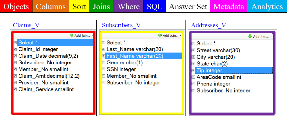
We understand that data in a data warehouse has tables, rows, and columns. In the old days, these were called files, records, and fields. In logical modeling terms, they are called relations, tuples, and attributes. The Nexus uses the logical model to allow users to see tables and all other tables in the relationship. Then, the Nexus builds the SQL with each click of the user's mouse.
First, Second and Third Normal Form
The process of placing columns in the correct tables is called normalization. There are three major forms of normalization, and they are first, second, and third normal form.
A Primary Key is usually the first column in the table and it is always unique and not null. The other columns in the table relate to the Primary Key.
A Foreign Key is a normal column in the table that is the connector to another table's Primary Key, and thus they have a join relation. Think of the Employee_Table having a Primary Key of Employee_No and a Foreign key of Dept_No, and this table has a relation to the Department_Table that has a Primary Key of Dept_No.
First Normal Form (1NF) means that columns (attributes) must not repeat within a table. No repeating groups such as Monday_Sales, Tuesday_Sales, etc.
Second Normal Form (2NF) means that all columns relate to the entire Primary Key and not just a portion of the Primary Key. Columns can also relate to each other, such as Dept_No and Department_Name, by both being in the table. Tables with a single column Primary Key are always in Second Normal form.
Third Normal Form (3NF) means all columns must relate to the Primary Key and not to each other. This is often termed that all columns must relate to the key, the whole key, and nothing but the key so help you Codd.
Quiz – Choose that Normalization Technique
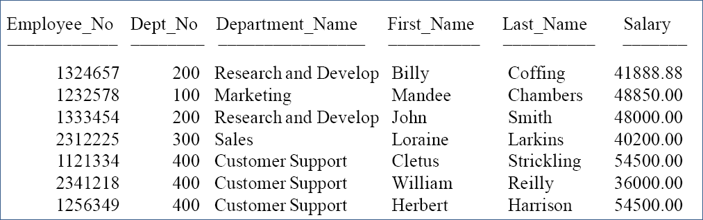
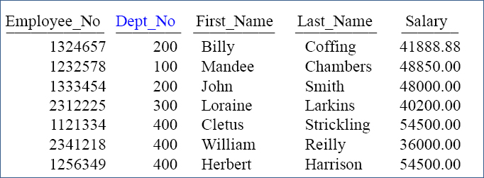
Below is a table with rows and columns. What form of normalization is this example?
Primary Key
Answer to Quiz – Choose that Normalization Technique
Below is a table with rows and columns. What form of normalization is this example?
Primary Key
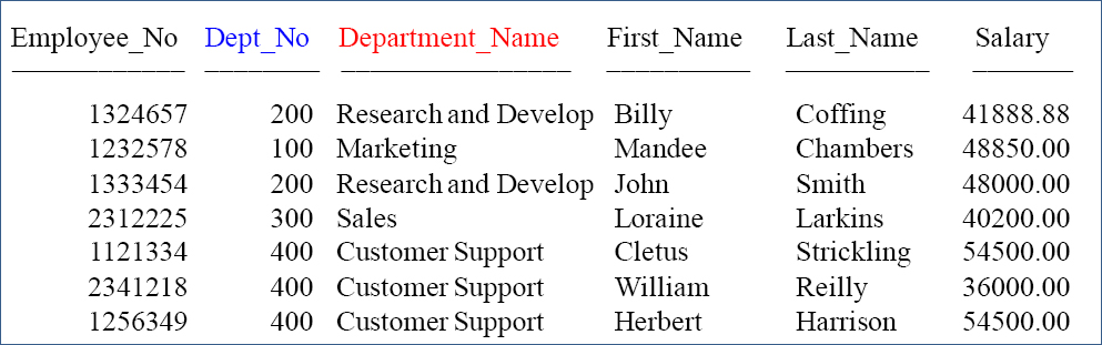
This is second normal form (2NF)
The reason is that although all columns relate to the Employee_No, the Department_Name is also a direct relation of the Dept_No.
Quiz – What Normalization is it Now?
Primary Key Foreign Key

Primary Key
| Dept_No | Department_Name | Budget |
100 |
Marketing |
500000.00 |
200 |
Research and Develop |
550000.00 |
300 |
Sales |
650000.00 |
400 |
Customer Support |
500000.00 |
Above are tables with rows and columns. What form of normalization is this example?
Answer to Quiz – What Normalization is it Now?
Primary Key Foreign Key
Primary Key
| Dept_No | Department_Name | Budget |
100 |
Marketing |
500000.00 |
200 |
Research and Develop |
550000.00 |
300 |
Sales |
650000.00 |
400 |
Customer Support |
500000.00 |
Both table are in third normal form (3NF). All columns relate to the Primary Key, the whole key, and nothing but the key. Tables are joined via the Dept_No column that resides in both tables.
The Employee_Table and Department_Table can be Joined
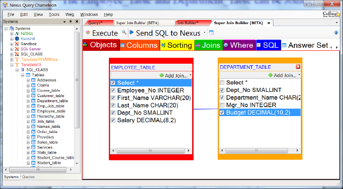
The Nexus knows the join relationships between tables. Above, you can see that the user sees both tables, and they have clicked on the columns they want on the report. Turn the page and see the SQL that Nexus has built for them. Tables with a Primary Key-Foreign Key relationship can be joined together with SQL.
The Employee_Table and Department_Table Join SQL
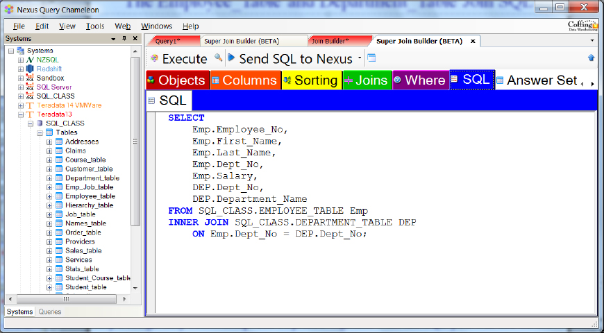
Tables with a Primary Key-Foreign Key relationship can be joined together with the SQL you see above in the SQL tab of Nexus. Tools like Nexus can help users dramatically because having Nexus navigate the table relationships allows users to visually see the tables and their relationships and then let Nexus build the SQL.
The Extended Logical Model Template
You communicate with the end user community to see how they will access the data, and you run queries on the data to understand the data demographics. The Logical Data Model will be the input to the Extended Logical Data Model. The Extended Logical Data Model will be input to the Physical Data Model.
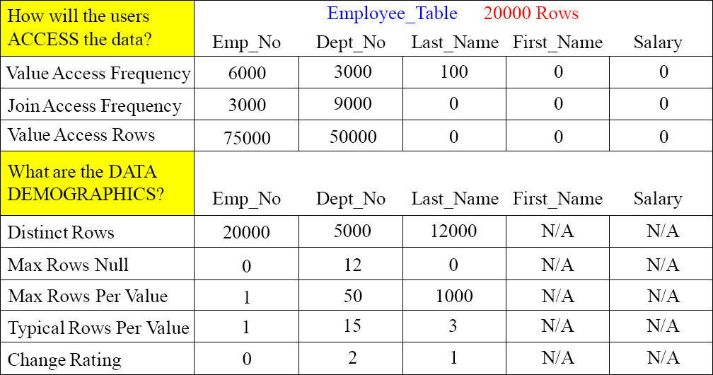
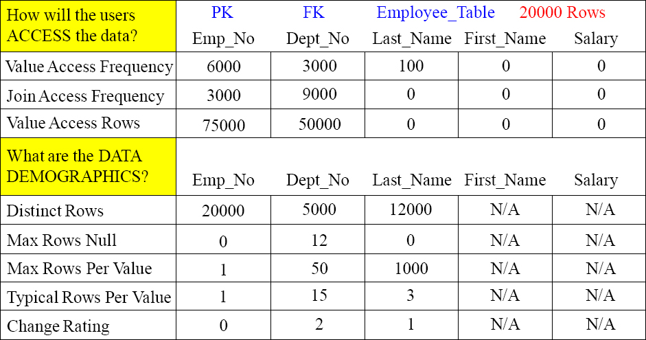
User Access is of Great Importance
The first and most important part of a Teradata Physical Model is choosing the primary index of each table and any secondary indexes. The Primary Index is the most important decision. If users are not querying a column, then there is no reason to make it a primary or secondary index. Choosing a great primary index makes access using that column a single AMP operation. When you join two tables using the primary index, no data movement is involved.
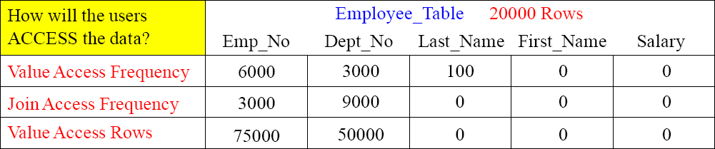
Value Access Frequency - How often will this column be accessed in the SQL WHERE clause?
Join Access Frequency - How often will this column be used as the join column to another table?
Value Access Rows - The number of rows that will be accessed multiplied by the frequency at which the column will be used.
The Access part of the template is important to understand how users will access data.
User Access in Layman's Terms
We use these templates to pick the best Primary Index for a table. We also use them to examine if a Secondary Index is appropriate if the column is not used as the Primary Index.
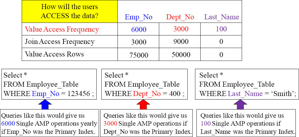
Getting as many Single AMP Retrieves by using the Primary Index in the WHERE clause is the essence of design in a Teradata system. Only one AMP is used, and only one block is transferred into the AMP's FSG Cache.
User Access for Joins in Layman's Terms
We use templates to pick the best Primary Index for a table. Joins are important in this decision.
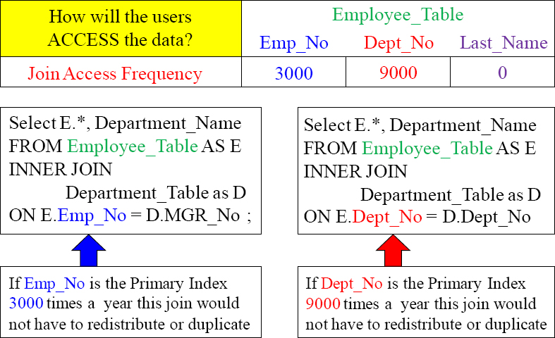
Joins are the most taxing process in Teradata because all matching rows must be joined on the same AMP. So, most of the time, Teradata will redistribute one or both of the tables or duplicate the smaller table temporarily in spool to enable the join to happen. A brilliant technique is to find out the join criteria, and make those columns the Primary Index. No data has to move because the matching rows are already on the same AMP.
The Nexus Shows Users the Table's Primary Index
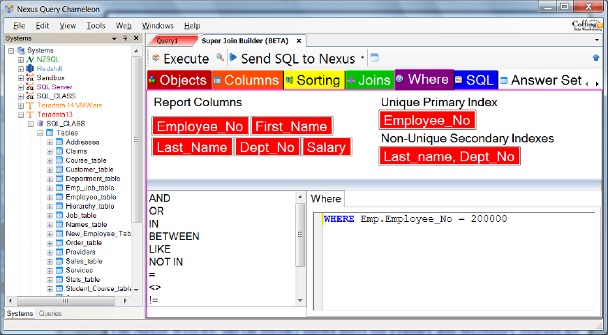
Accessing tables and views using the Primary Index is vital to a successful Teradata implementation. The Nexus WHERE tab (in purple) shows users the Primary and Secondary Indexes for all tables. Nexus also shows the underlying indexes when users are accessing views. Users can point and click on the index, and Nexus builds the SQL.
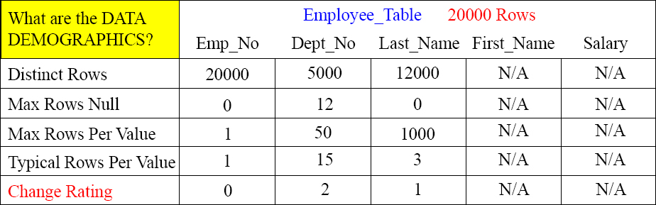
Data Demographics Tell Us if the Column is Worthy
There are Unique and Non-Unique Primary and Secondary Indexes. Data demographics give us a picture of the data so we can tell if the column is worthy of an index.
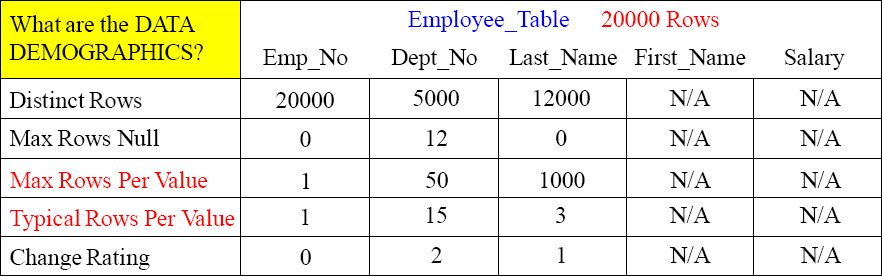
Distinct Rows – How many distinct values are in this column? Will it spread the data evenly?
Max Rows Null – How many rows in this column are Null?
Max Rows Per Value – What value is the most popular and how many values does it have?
Typical Rows Per Value – What's the typical amount of duplicate values for the column? Looking at the Max Rows Per Value Vs. the Typical Rows Per Value shows us the skew factor.
Change Rating – How often will the column be updated and the value change in this column? If the column changes values all the time, it must be eliminated as a primary index candidate.
Data Demographics – Distinct Rows
The key to Distinct Rows is to first see if the column is unique. If it is unique, we can then consider it for a Unique Primary Index or a Unique Secondary Index.

Distinct Rows – How many distinct values are in this column? Will it spread the data evenly?
If the rows are not unique, we can still get an idea if it will spread the data evenly if it is chosen as a Primary Index. We need to make sure that there are more distinct values than AMPs if this is to be considered a Primary Index candidate.
Above, we can see that this table has 20000 rows and that Emp_No has 20000 distinct rows. So, we know it is a unique column. Dept_No has only 5000 distinct values, so it is still a candidate.
Data Demographics – Distinct Rows Query
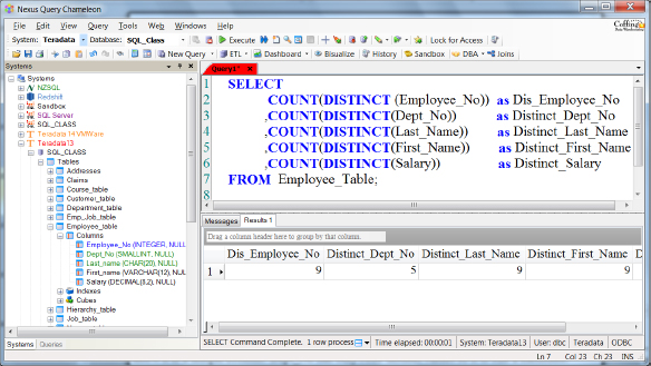
Above is a query you can run to get the distinct values for each column.
Data Demographics – Max Rows Null
The key to Max Rows Null is to get an idea if the column contains Null values. If there are no Null values, we should specify NOT NULL in the table CREATE statement. If there are Null values, then those will hash to a single AMP if the column is chosen as the Primary Index thus potentially causing skew. If there are more than one Nulls, then we can't have that column become a Unique Primary or Unique Secondary Index.
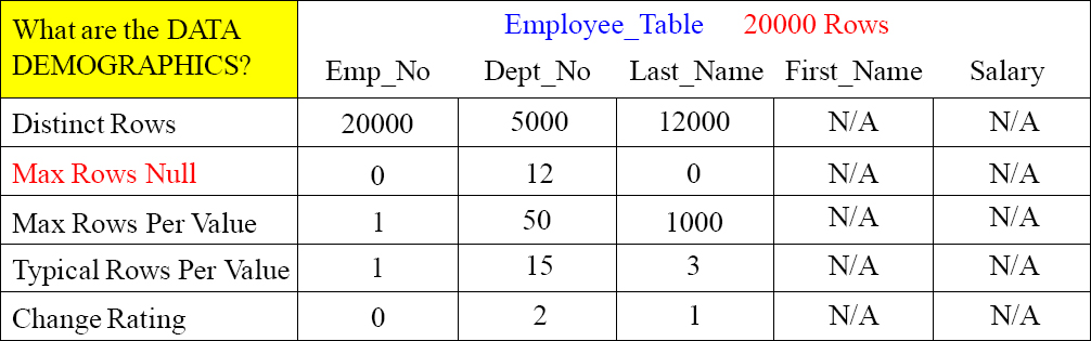
A few Nulls are not a big problem, but a lot of Null values are a problem as they could cause skew if the column is chosen as the Primary Index.
Data Demographics – Max Rows Null Query

Above is a query you can run to get the Max Rows Null values for each column.
Data Demographics – Max Rows Per Value
Max Rows Per Value tells us many things. First of all, it lets us know if the column is a candidate for a Unique Primary Index or a Unique Secondary Index. Emp_No has only one Max Rows Per Value, so it is unique. The next thing the Max Rows Per Value tells us is if there will be a spike in our distribution if this column is a Primary Index. For example, Last_Name has a Max Rows Per Value of 1000. This means that a Last_Name like ‘Smith’ has 1000 entries. This is a huge spike because if Last_Name is the Primary Index, then one AMP will hold all 1000 Smiths.
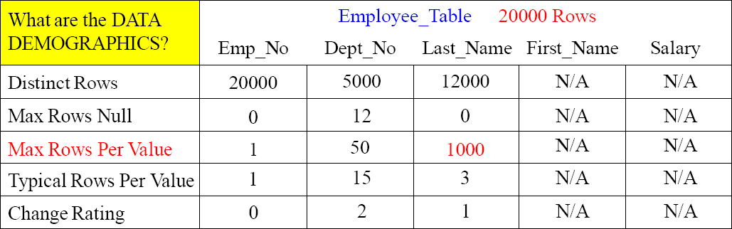
The Max Rows Per Value should also be compared to the Typical Rows Per Value to see just how skewed the data will be if the column is chosen as the Primary Index. Comparing these two values will let you know if there will be a spike on one AMP, or if that generally the data will be distributed fairly evenly.
Data Demographics – Max Rows Per Value
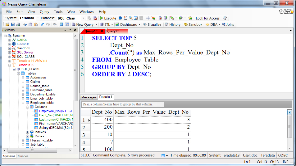
Above is a query you can run to get the Max Rows Per Value for each column. The query above will give you the TOP 5 Max Rows Per Value.
Data Demographics – Typical Rows Per Value
Typical Rows Per Value tells us many things. First of all, it lets us know if the column is a candidate for a Unique Primary Index or a Unique Secondary Index. It can also be compared to the Max Rows Per Value to show how evenly or how skewed the data will be if this column is chosen as the Primary Index. It is also a guideline for a Secondary Index. It is important that a Non-Unique Secondary Index is strongly selective. In other words, if there are typically a lot of duplicates, then it is weakly selective. It is like asking everyone in the room if they breathe.
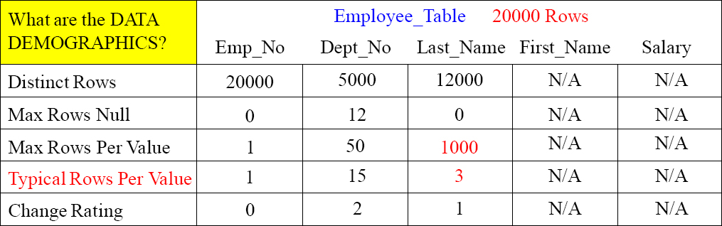
Notice Last_Name has a Typical Rows Per Value of three and a Max Rows Per Value of 1000. This means it might not be a good candidate as a Primary Index because of the spike of 1000, but it has a low Typical Rows Per Value which means it is strongly selective as a Non-Unique Secondary Index (NUSI). Only three rows per Last_Name is useful for a NUSI search.
Typical Rows Per Value – Query 1 (Median)

Above is a query you can run to get the Typical Rows Per Value for each column. The column we chose to get the Typical Rows Per Value was the Product_ID column in the Sales_Table. All you need to do is change the table name and the column name and you are all set. This is also referred to as the Median Value.
Typical Rows Per Value – Query 2 (Median)
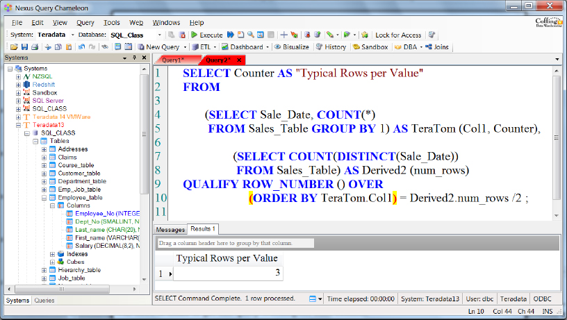
Above is a query you can run to get the Typical Rows Per Value for each column. The column we chose to get the Typical Rows Per Value this time was the Sale_Date column in the Sales_Table. I wanted to show you two examples so you could better understand the changes you will need to make to get this query working for each column. Just replace the table name and the column you want to choose and you are all set. This is also referred to as the Median Value.
Row_Number With Qualify to get the Typical Rows Per Value
SELECT Counter AS “Typical Rows per Value”
FROM
(SELECT Product_ID, COUNT(*)
FROM Sales_Table GROUP BY 1) AS TeraTom (Col1, Counter),
(SELECT COUNT(DISTINCT(Product_ID))
FROM Sales_Table) AS Derived2 (num_rows)
QUALIFY ROW_NUMBER () OVER
(ORDER BY TeraTom.Col1) = Derived2.num_rows /2 ;
Typical Rows Per Value
7
The query above retrieved the typical rows per value for the column Product_ID.
SQL to Get the Average Rows Per Value for a Column (Mean)
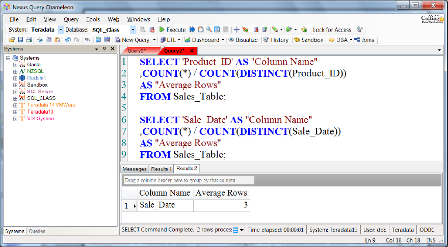
Above, is a query you can run to get the Average Rows Per Value for each column. The column we chose to get the Average Rows Per Value this time was the Product_ID and then the Sale_Date column in the Sales_Table. I wanted to show you two examples so you could better understand the changes you will need to make to get this query working for each column. Just replace the table name and the column you want to choose, and you can get the Mean Value.
Getting the Average Values Per Column
SELECT ‘Product_ID’ AS “Column Name”
,COUNT(*) / COUNT(DISTINCT(Product_ID)) AS “Average Rows”
FROM Sales_Table;
| Column Name | Average Rows |
| 3 |
The query above retrieved the average rows per value for the column Product_ID.
Data Demographics – Change Rating
Change Rating is a rule of thumb metric that you have to guesstimate sometimes. How often will a column be updated and change its value? If a column changes values a lot, then it will be too disruptive to be a Primary Index. A Primary Index shouldn't change very often. A Secondary Index can change a little more, but even that should have a low change rating. Each time a Primary Index column changes, the row needs to move to a new AMP, and each secondary index subtable needs to be updated. That can be too much overhead.
Notice that each change rating is pretty low, so each of these could be a Primary or Secondary Index candidate.
Factors When Choosing Teradata Indexes
- How will Teradata use the index?
- How much space will the index require?
- What type of table is it (Set, Multiset, Staging, Queue, Temporal, PPI, Columnar)?
- How many rows are in the table?
- How many columns are in the table?
- What are the table protection types?
- Does the table have referential integrity?
- What column(s) are most frequently used in the WHERE clause to access rows in the table?
- What is the number of distinct values in a column?
- What are the maximum rows per value Vs. the typical rows per value?
- Is the table accessed via a Full Table Scan, through column values by a Join?
- How many tables will join to this table on average?
- Is the table used for DSS, reports, batch, OLTP, analytics, Ad Hoc queries or a combination?
- What is the number of INSERTS and when will they occur?
- What is the number of DELETEs and when will they occur?
- What is the number of UPDATEs and when will they occur?
- How often will an UPDATE cause a column to change values?
- How are transactions written (single statement, multi-statement)?
- What level and type of locking will a query or transaction require (Access, Write, Read)?
- How long will a transaction hold locks?
- How normalized is the data model?
Finding Table Sizes
SELECT Databasename
,TableName
,SUM(CurrentPerm) as Current_Perm
,SUM(PeakPerm) as Peak_Perm
FROM DBC.Tablesize
WHERE DatabaseName LIKE ‘SQL%’
GROUP BY 1, 2
ORDER BY 1, 3 DESC, 2;
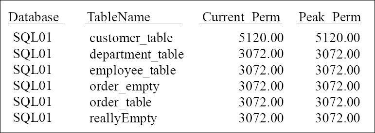
You can now keep track of the size of tables.
Finding Skew in The Tables in a Database
SELECT
Vproc
,CAST (TableName AS CHAR(20))
,CurrentPerm
,PeakPerm
FROM DBC.TableSizeV
WHERE DatabaseName = ‘SQL_Class’
ORDER BY TableName, Vproc ;
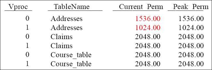
A Vproc is an AMP. There are only two AMPs on this system and they are referred to as Vproc 0 and Vproc 1. Notice that the Addresses table has skew because of the Current_Perm for Vproc 0 (1536) is different than Vproc 1 (1024).
Finding Skew in a Table
SELECT
Vproc
,TableName (CHAR(15))
,CurrentPerm
FROM DBC.TableSizeV
WHERE DatabaseName = ‘SQL_Class’
AND TableName = ‘Addresses’
ORDER BY 1 ;
| Vproc | TableName | Current_Perm |
0 |
Addresses |
1536.00 |
1 |
Addresses |
1024.00 |
A Vproc is an AMP. There are only two AMPs on this system and they are referred to as Vproc 0 and Vproc 1. Notice that the Addresses table has skew because of the Current_Perm for Vproc 0 (1536) is different than Vproc 1 (1024).
Display the Distribution of a Column Per AMP
SELECT
HASHAMP (HASHBUCKET
(HASHROW (Product_ID))) AS “AMP #”
,COUNT(*)
FROM SQL_Class.Sales_Table
GROUP BY 1
ORDER BY 1 ;
| AMP# | Count(*) |
| 0 | 14 |
| 1 | 7 |
A Vproc is an AMP. There are only two AMPs on this system and they are referred to as Vproc 0 and Vproc 1. Notice that the Sales table has skew because of the Count(*) for the Primary Index of Product_ID with 14 rows for AMP 0 Vs. 7 rows for AMP 1.
Primary Index Data Demographics Candidate Guidelines
The Primary Index Candidate Guidelines should consider the Primary Key of a table and any Unique columns. The candidate should also be any single column with High Distinct Values, a low maximums for Null values, and should provide good distribution. So, it should have a Typical Rows that is close to the Max Rows so there are no spikes in the AMPs.

Primary Index Access Considerations
There are three important functions of the Primary Index. They are:
- Data Distribution
- Fast Data Access
- Joins
What should be your priority as a Teradata expert? All three are important, but how should you approach your decision? The next page will reveal the answer.
Of the three important functions listed above, which one do you think is the most important consideration? List from first to last which priority should be considered first, second and third.
1) _____________
2) _____________
3) ______________
Then turn the page!
Answer -Three Important Primary Index Considerations
Below, are the Tera-Tom priorities for choosing the column to be the table's Primary Index,.
- Joins – It is the joins of tables that are the most taxing on a Teradata system, so understanding how to enhance joins can do more for your system than anything else. This is your biggest opportunity! How does Teradata join five tables together? Teradata always joins tables two at a time because the matching rows must be on the same AMP. If the rows are not on the same AMP, Teradata must redistribute or duplicate to get the matching rows together. The only thing that designates where an AMP is physically is the Primary Index. A brilliant move is to consider tables that are joined together often, and to make the join columns (PK/FK) the primary index on both tables. This will enhance the joining process to perfection.
- Data Access – Using the Primary Index in your SQL WHERE clause is lightning fast for data retrieval, but you have the option of quick access with secondary indexes (especially a Unique Secondary Index). That is why joins should be your first consideration. However, if you have hundreds of users who need split second response times (called tactical queries) to certain tables, then Data Access is your top opportunity to make that happen.
- Data Distribution – Most newbies to Teradata focus on data distribution as their most important consideration because it is the first and most fundamental thing they learn about the Primary Index. What is interesting here is that you should consider the joins first, and then the data access second. But after that, if the column you are considering will cause bad data distribution, then you have to take it off the table. Data Distribution is very important, but don't let it bias you and look at it last!
The First Step is to Pick All Potential Primary Index Columns
Place an UPI or a NUPI for any column that you consider a possible Primary Index candidate. UPI stands for Unique Primary Index and NUPI for Non-Unique Primary Index.
UPI/NUPI Candidate? ________ ________ ________ ________ ________
The First Step is to Pick All Potential Primary Index Columns
Place an UPI or a NUPI for any column that you consider a possible Primary Index candidate. UPI stands for Unique Primary Index and NUPI for Non-Unique Primary Index.

UPI/NUPI Candidate? UPI NUPI NUPI
The 2nd Step is to Pick All Potential Secondary Indexes
Place an USI or a NUSI for any column that you consider a possible Secondary Index candidate. USI stands for Unique Secondary Index and NUSI for Non-Unique Secondary Index.

UPI/NUPI Candidate? UPI NUPI NUPI
USI/NUSI Candidate? ________ ________ _______
Answer to 2nd Step to Picking Potential Secondary Indexes
Place an USI or a NUSI for any column that you consider a possible Secondary Index candidate. USI stands for Unique Secondary Index and NUSI for Non-Unique Secondary Index.

UPI/NUPI Candidate? UPI NUPI NUPI
USI/NUSI Candidate? USI NUSI NUSI
Now it is time to choose the Primary and Secondary Indexes
It is time to make a first run at choosing the Primary and Secondary Indexes. Ask yourself:
1) Will this table do a lot of joins or will users need to access just this table fast? Which will happen more and be a bigger priority?
2) Is the table big or small? If it is small then joins won't be a problem. If it is big they could be. How often will users need to access just this table in sub second time?
3) What does the data distribution look like? Are there a lot of nulls? Will the data skew badly?
4) How often will the data change for this column? Eliminate it as a Primary Index candidate if it will change a bit, and eliminate it as a Secondary Index if it will change somewhat often.
5) A Unique Secondary Index is usually a great choice for Access, but a Non-Unique Secondary Index must be strongly selective. That means there must be many different distinct values.
6) Time to now decide on your Primary and Secondary Indexes.
Turn the page and choose! Then, we will compare on our choices.
3rd Step is to Picking your Indexes
It is now time to pick your Primary Index and any Secondary Indexes. Good luck! We will show you our choices on the following page.

UPI/NUPI Candidate?
USI/NUSI Candidate?
Our Index Picks

Index Candidate? USI NUPI
This was a tough call. Because of the large amount of joins and the reasonable distribution, we chose Dept_No as our Non-Unique Primary Index (NUPI) and Emp_No as our Unique Secondary Index (USI). Switching these could have also worked out, but now our joins will be fast and all access using the Emp_No column to search will be a fast two AMP retrieve.