
Chapter 3 - Teradata - The Cold Hard Facts
“Time is the coin of your life. It is the only coin you have, and only you can determine how it will be spent. Be careful lest you let other people spend it for you.”
Teradata Parallel Processing
Each AMP holds a portion of the rows for every table in the system.
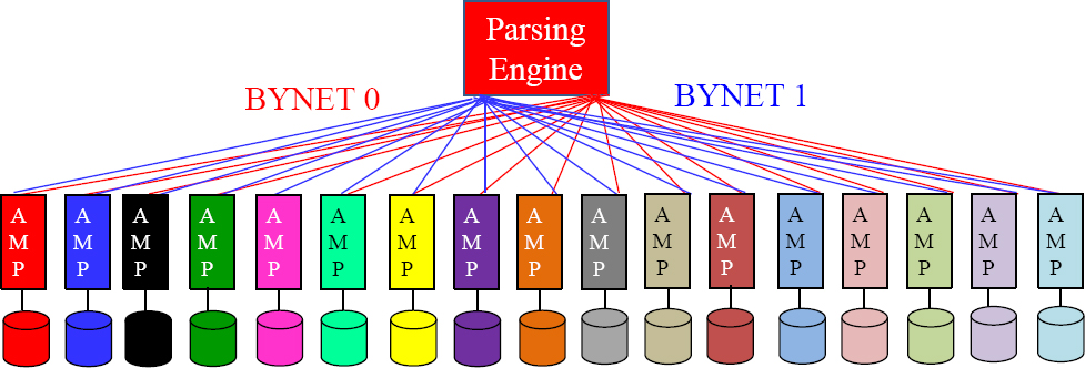
Teradata was born to be parallel. When a user queries a system, they logon to a Parsing Engine for the entire session. The Parsing Engine checks the User's SQL syntax, their Access Rights for security purposes. Then, it comes up with a plan for the AMPs to retrieve the data. The Parsing Engine passes the plan to the AMPs over one of the two BYNET networks, and the AMP's work simultaneously in parallel to retrieve the data.
We know that the “Achilles Heel” of Teradata is the movement of blocks from disk to memory, but the great news is that Teradata's parallel processing moves blocks simultaneously. The more AMPs the system has the more power, so realize it is the parallel processing that makes Teradata all powerful when performing massive queries.
Each Table has a Primary Index that is Unique or Non-Unique

Each Teradata table has only one Primary Index and it is either a Unique Primary Index (UPI) or a Non-Unique Primary Index (NUPI). The Primary Index is established when the table is created inside the CREATE Table statement. It is the Primary Index column that will be used by Teradata to distribute the rows among the AMPs.
The Hash Map Determines which AMP will own the Row
Every row is run through a math formula, and the result is the “Row Hash”. This alone, in conjunction with the Hash Map, determines which AMP will hold the row.
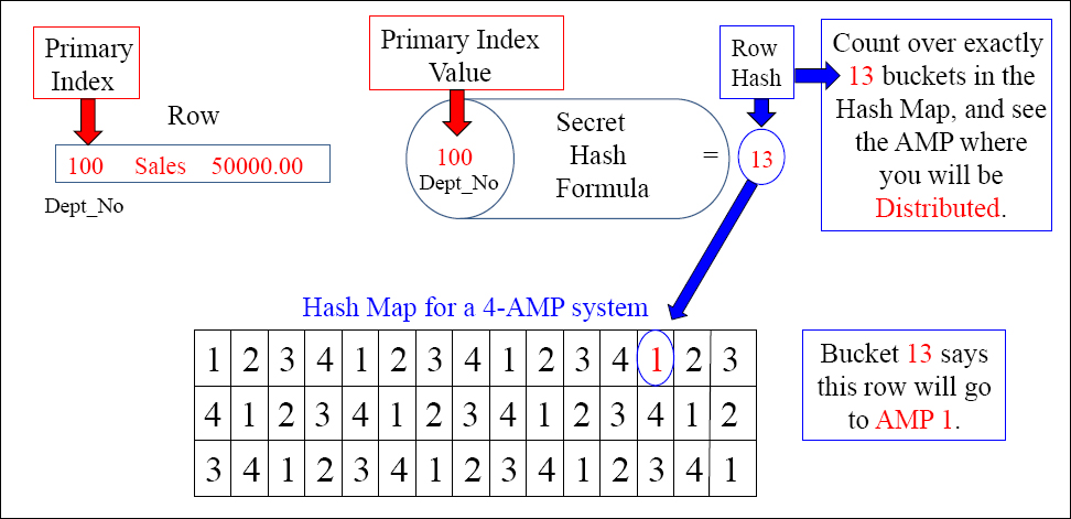
Teradata uses one secret “Hash Formula” that runs a math formula on the Primary Index value of each row. The hashing of the row results in an answer called the “Row Hash”. This alone, in conjunction with the system's hash map, determines which AMP holds the row. The Parsing Engine can rerun the Hash Formula again to quickly find the row.
A Unique Primary Index Spreads the Data Evenly

The Row Hash is the result of the Primary Index value going through the Hash Formula. It will stay with the row forever.
The Department_Table has a Unique Primary Index (UPI) on Dept_No. The rows are spread evenly across the AMPs. Take notice of the Row Hash in front of each row. When the row is hashed, the resulting Row Hash sticks with the row like glue forever.
The AMP Adds a Uniqueness Value to Create the Row-ID
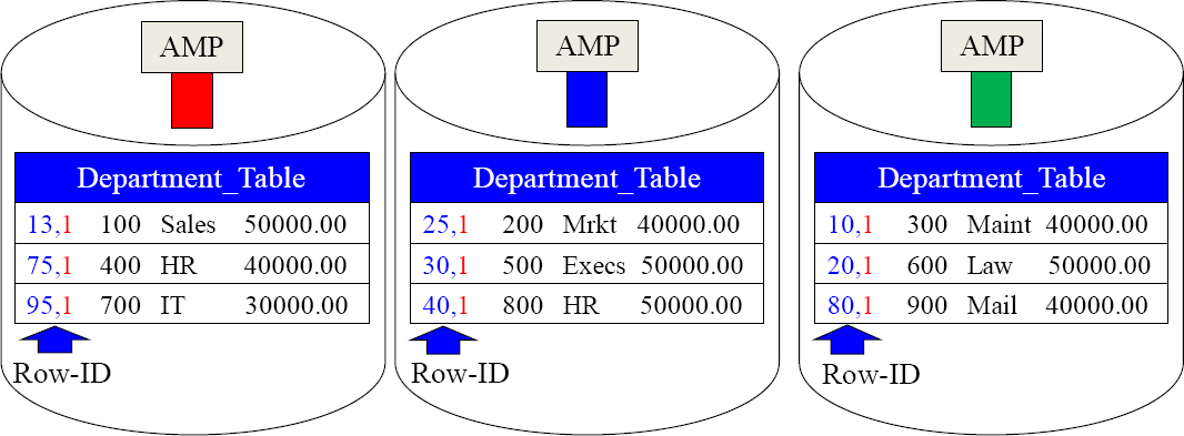
The Row Hash is the result of the Primary Index value going through the Hash Formula. The AMP adds a Uniqueness Value and the combination of the Row Hash and the Uniqueness Value form a Row-ID.
Notice that each AMP adds a Uniqueness Value to the row hash, and this forms the Row-ID. The Row-ID is unique within a table. Why are all the Uniqueness Values equal to a one (1)? Each Dept_No is unique, so each “Row Hash” is unique, so a Uniqueness Value of one (1) is entered. AMPs sort their rows by the Row-ID.
Each AMP Sorts Their Tables by the Row-ID
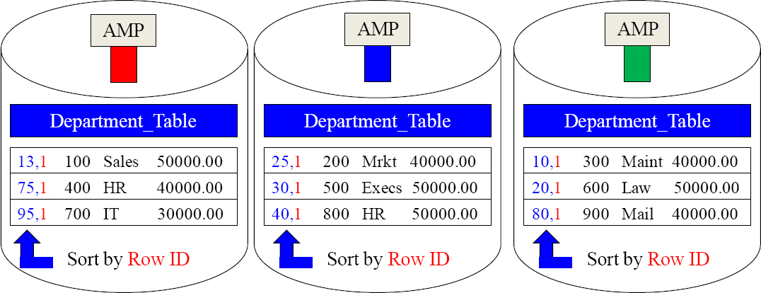
How does each AMP sort the rows they own? By the Row-ID.
Each AMP sorts their rows by the Row-ID. Now, an AMP can look up a specific row like a person looks up a name in a phone book. People can easily use a phone book because it is in alphabetic order. An AMP can quickly find rows using an index because its rows are in binary order. A person uses a phone book by looking in the middle and then moving up or down a group of pages until the search is satisfied. An AMP searches the same way, but using binary numbers to find a specific row hash quickly.
A Non-Unique Primary Index Skews the Data
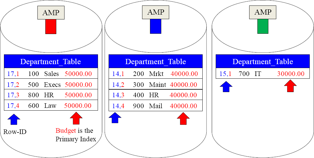
Because Budget was chosen as the Primary Index, and the Teradata hash formula is consistent, all like values go to the same AMP. Notice that all of the budgets of 50,000.00 went to AMP 1. The 40,000.00 budgets all went to AMP 2, and the only row with a 30,000.00 budget went to AMP 3. The data is skewed. Also, notice the Row Hash values and the increasing Uniqueness ID for budgets with the same value.
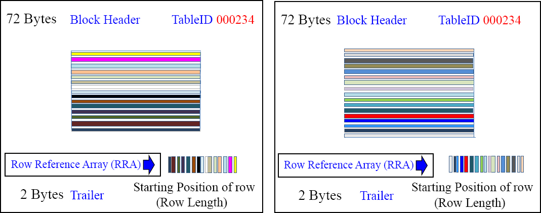
Comparing the Same Table with Different Primary Indexes
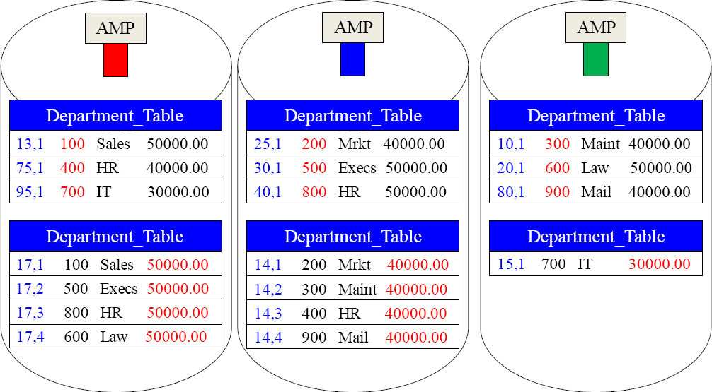
The Department_Table is laid out twice, but with a different Primary Index. The red colors denote the table's Primary Index, and the blue colors denote the Row-ID. The top example uses a Unique Primary Index (UPI) to distribute data evenly. But, the bottom example uses Budget as a Non-Unique Primary Index (NUPI), and the data is skewed.
Unique Primary Index Queries are a Single AMP Retrieve

SELECT*
FROM Department_Table
WHERE Dept_No = 100 ;
The above query uses the Unique Primary Index (UPI) on Dept_No in the WHERE clause of the SQL. This results in a “Single AMP retrieve”. Only AMP 1 is contacted to retrieve the row. The Parsing Engine distributes the data by hashing the Primary Index value with a “Hash Formula”, so the Parsing Engine's plan is to reengineer that process and the BYNET only contacts AMP 1. Give Teradata any Primary Index value for a table, and it knows which AMP has that row by rerunning the “Hash Formula”.
A Non-Unique Primary Index is also a Single AMP Retrieve
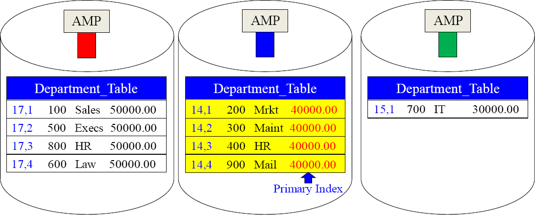
SELECT * FROM Department_Table
WHERE Budget = 40000.00 ;
The above query uses a Non-Unique Primary Index (NUPI) on the column Budget in the WHERE clause of the SQL. This also results in a Single AMP retrieve. Only AMP two is contacted to retrieve the rows. The Parsing Engine distributes the data by hashing the Primary Index value, so the Parsing Engine's plan is to reengineer this process and contact only the proper AMP. AMP two brings back all qualifying rows.
Teradata has a No Primary Index Table called a NoPI Table
CREATE TABLE Department_Table
(Dept_No INTEGER,
Dept_Name CHAR(20),
Budget DECIMAL(10,2))
NO PRIMARY INDEX ;
NoPI
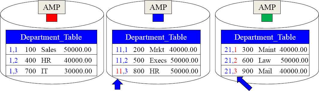
Each AMP is assigned a Row Hash and then it merely increments its Uniqueness Value
A NoPI Table has no primary index. A NoPI table guarantees even distribution. It still has a Row-ID. How? Each AMP is assigned a Row Hash, and then, for every row the AMP receives, it increments the Uniqueness Value. A NoPI table is most often used as a loading staging table or with a columnar designed table. Each row is appended quickly. Distribution is always random, but even, so as a staging table it is quicker to load.
There are Normal Tables and then There are Partitioned Tables
The table above is a partitioned table, which means the AMPs are ordered NOT to sort their rows by Row-ID, but instead to sort them by the partition. This is referred to as a Partitioned Primary Index table or PPI table. The only difference between a PPI table and a normal table (Non-Partitioned Primary Index) or (NPPI), is how the AMPs sort their rows. The example above has each AMP sort their rows by month of Order_Date.
A Visual of One Year of Data with Range_N per Month
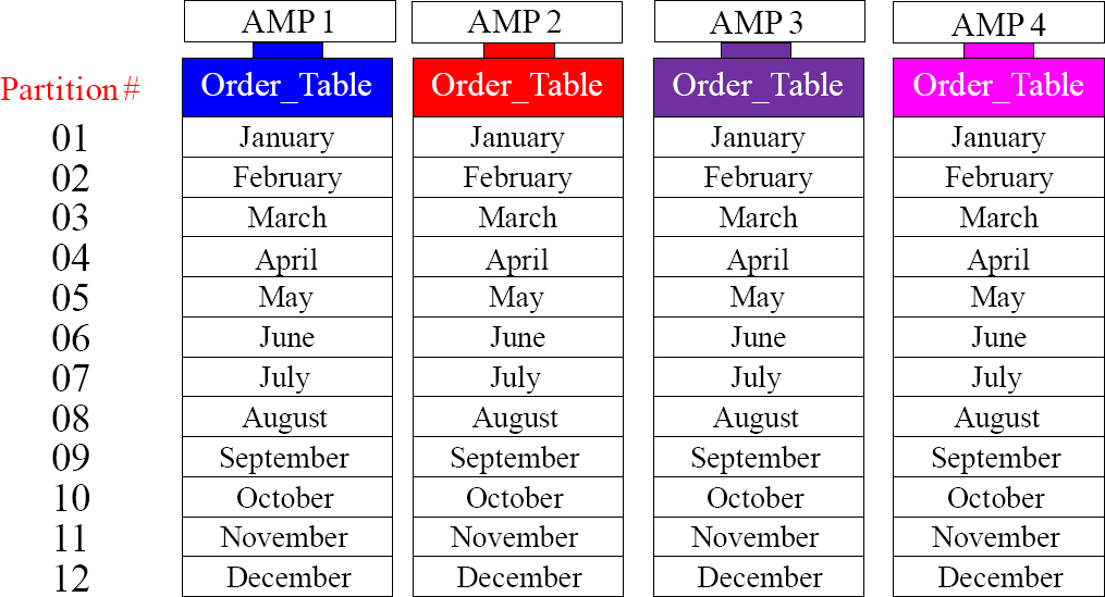
Each AMP above sorts their rows by Month (of Order_Date), which really means the rows are first sorted by the Partition Number and then by Row-ID within the partition. The combination of Partition Number and Row-ID is called the Row-Key. A normal table has AMPs sort their rows by Row-ID, but a PPI table sorts by Row Key.
Partitioning is Designed to Eliminate the Full Table Scan
SELECT * FROM Order_Table
WHERE EXTRACT (Month) From Order_Date = 10 ;
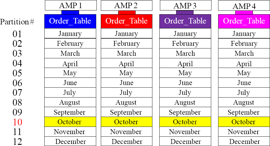
The query above performs an All-AMP retrieve, but from a single partition. It has NOT done a Full Table Scan. This is a major concept around Physical Database Design!
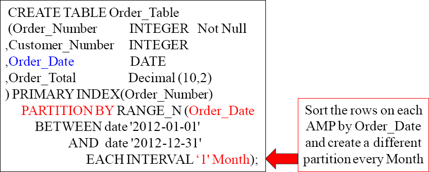
A Partition # and Row-ID = Row Key
CREATE TABLE Order_Table
(Order_Number INTEGER
,Customer_Number INTEGER
,Order_Date DATE
,Order_Total Decimal (10,2)
) PRIMARY INDEX(Order_Number)
PARTITION BY RANGE_N
(Order_Date BETWEEN
date ‘2013-01-01’ AND date ‘2013-12-31’
EACH INTERVAL ‘1'Month);
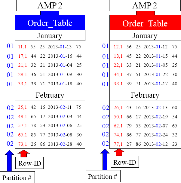
A Partitioned Table (PPI) is sorted on each AMP by the Row-Key.
Above, is Partition # 1 (January) and Partition # 2 (February). Inside each partition, you can see the Row-ID. The Partition # combined with the Row-ID is called the Row Key.
An AMP Stores its Rows Sorted in only Two Different Ways

An AMP stores its rows sorted by the Row-ID or the Row Key. A normal table sorts by the Row-ID and a Partitioned Table (PPI table) sorts on the Row Key (Partition # + Row-ID). You will soon find out exactly why this is done and the true meaning of Physical Database Design! These are the two ways AMPs sort data on disk.
AMPs Moves Their Data Blocks into Memory to Read/Write

Rows of a table can't be read on disk. Rows are merely stored on disk in data blocks. When a Full Table Scan (for example) needs to read, all rows of a table the AMP's will simultaneously move their data blocks into their dedicated memory.
Most Taxing thing for an AMP is Moving Blocks into Memory

Once the Table Header and the Data Block are inside an AMP's Memory, the AMP can read. The most taxing thing for an AMP to do is to move blocks from disk to memory.
Rows are Stored in Data Blocks which are stored in Cylinders
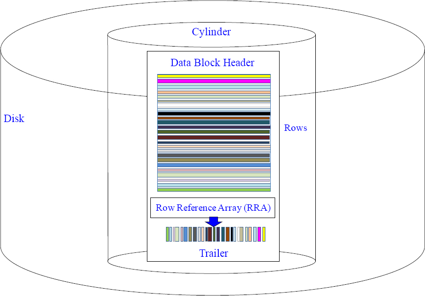
Above, you see many rows of the same table stored in a data block. You can have many data blocks stored in a cylinder, and an AMP owns thousands of cylinders.
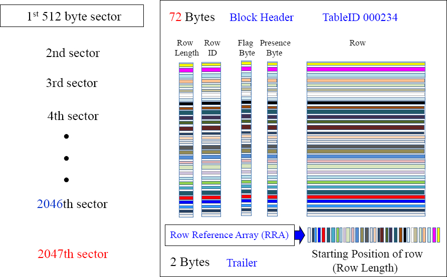
Rows for an AMP Stored Inside a Data Block in a Cylinder

This is a real data block that contains the overhead in front of each row. This data block, among other data blocks, will reside inside a cylinder. The rows are sorted by Row-ID, so the AMP can read the Row Reference Array like a phone book to quickly find a row.
An AMP's Master Index is Used to Find the Right Cylinder
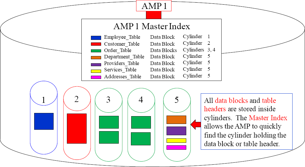
An AMP has thousands of cylinders. Inside each cylinder are data blocks where the AMP stores the rows of a table. The AMP's Master Index is always in memory, so it can easily locate the cylinder containing the data. Once the data block and table header are located and moved into memory, rows can then be processed.
The Row Reference Array (RRA) Does the Binary Search?
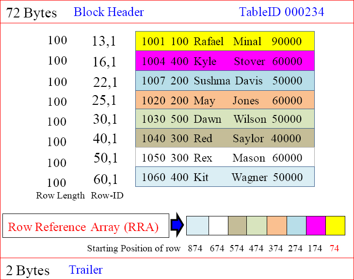
There is one Row Reference Array (RRA) inside each data block. This array shows the starting position of each data row. Now, the AMP can start in the middle of the RRA and look for a row's Row-ID and either find it or know to move up or down like you might use a phone book. The Row Reference Array is always in Row-ID order.
A Block Splits into Two Blocks at Maximum Block Size
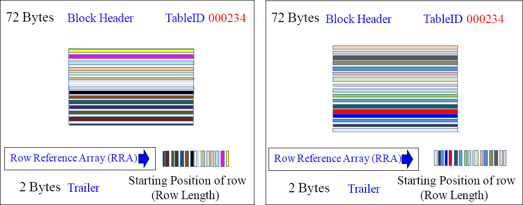
Once a block reaches the maximum block size (on an AMP), the AMP splits the block from one 255 sector block to two separate 127.5 sector blocks. Notice that we have the same total amount of rows, but now half the rows are in the first data block, and the other half of the rows are in the second data block. Notice that both blocks have the same TableID, and notice now there is a Block Header, Row Reference Array, and Block Trailer in both of the blocks. An AMP might have many blocks for a single table.
Data Blocks Maximum Block Size has Changed (V14.10)
The maximum block size (before a split) was 255 sectors (127.5 K), but now it is 2047 sectors (1 MB).
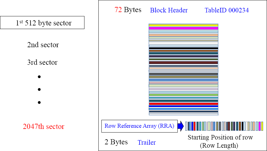
Prior to Teradata 14.10, the maximum block size is 255 sectors or 127.5 KB. Starting with Teradata 14.10, the maximum block size has been increased from 127.5 KB to approximately 1MB. The Max user-specifiable size is 2047 sectors.
The New Block Split with Teradata V14.10
In Teradata V14.10, once this block reaches the maximum block size (on this AMP), the AMP splits the block from one 2047 sector block to two separate 1023.5 sector blocks. Blocks can vary in size from 1 sector to the maximum size (255 or 2047). A maximum row size is 64,255 bytes. Rows can vary in size within the block.
The Block Split with Even More Detail in Teradata V14.10
As data is added, Teradata continues to grow the block one 512 byte sector at a time. Once the block grows to the maximum size, then Teradata will split the single block into two separate blocks. The default for the split is 2047 sectors or 1 MB.
Teradata V14.10 Block Split Defaults
Teradata 6700 EDW
Default Block Split
512 K

Teradata 2700 Appliance
Default Block Split
256 K

The maximum for all Teradata V14 data block splits are 2047 sectors or 1 MB, but the defaults differ based on whether or not it is an enterprise class system, or an appliance.
There is One Master Index and Thousands of Cylinder Indexes
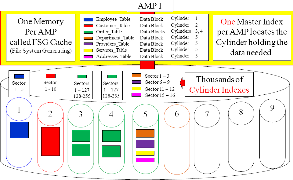
There is only one Master Index per AMP, and its purpose is to locate the cylinder that holds a particular data block or table header. Then, each cylinder has a Cylinder Index so the AMP can locate the exact location of a particular data block or table header.
Each Table has a 48-bit TableID
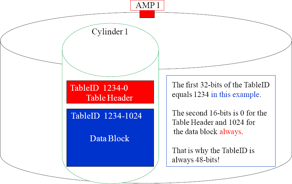
Both blocks in Cylinder 1 above are from the same table. The first 32-bits have the same value in 1234, but the second 16-bits identify Table Header vs. Data Block.