chapter three
identify & eliminate clutter
Every element we put in our graphs or on the pages and slides that contain them adds cognitive burden—each one consumes brainpower to process. We should take a discerning look at the elements we allow into our visual communications and strip away those things that aren’t adding enough informative value to make up for their presence.
This lesson is simple but the impact is huge: get rid of the stuff that doesn’t need to be there. We’ll illustrate and experience the power of doing so through a handful of targeted exercises in this chapter.
Let’s practice identifying and eliminating clutter!
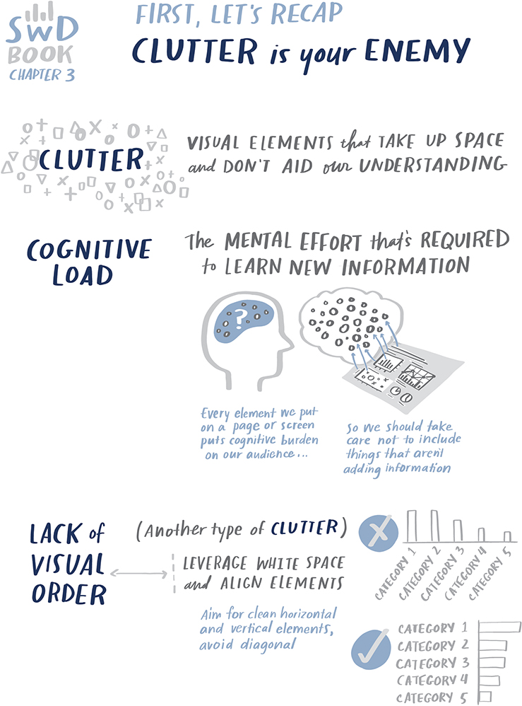
First, we’ll review the main lessons from SWD Chapter 3.


Exercise 3.1: which Gestalt principles are in play?
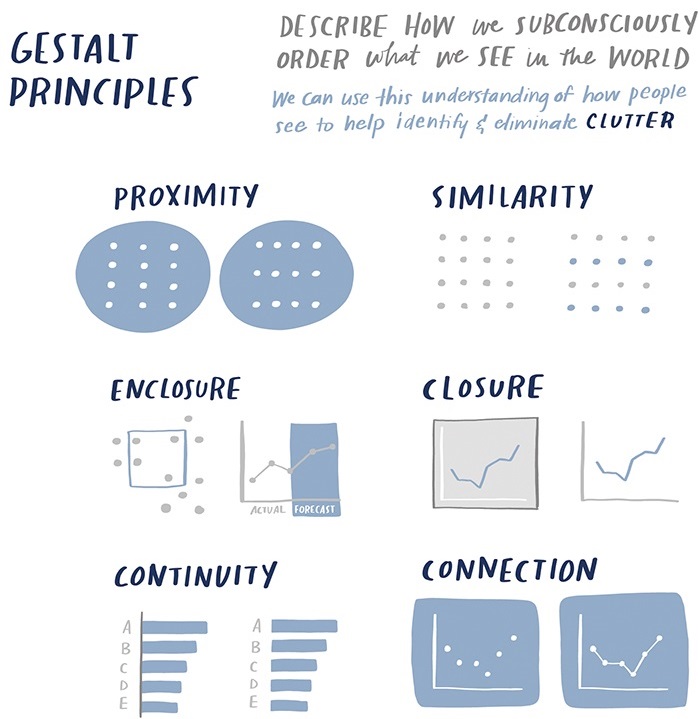
The Gestalt principles describe ways in which we subconsciously bring order to the things we see. SWD introduced six of these principles: proximity, similarity, enclosure, closure, continuity, and connection. We can use the Gestalt principles to make our visual communications easier for our audience to process by helping make the connections between the different elements we show more obvious. (If you aren’t familiar with these principles and don’t have SWD handy, we’ll review them in detail through the solution to this exercise.)
Consider the following visual, which illustrates actual and forecast market size (measured by total sales) over time for a class of pharmaceutical drugs. Which of the Gestalt principles mentioned above can you identify? Where and how are each used?
Solution 3.1: which Gestalt principles are in play?
I’ve made use of each of the six Gestalt principles in Figure 3.1. Let’s briefly discuss.

Figure 3.1 Which Gestalt principles are in play?
Proximity: Proximity is used in a number of ways. The physical closeness of the y-axis title and labels indicates to us that those elements are to be understood together. The close proximity of the data labels to the data markers makes it clear that those relate to each other.
Similarity: Similarity of color (orange and blue) is used to visually tie sparing words in the text at the top to the data points in the graph that those words describe.
Enclosure: The light grey shading on the right side of the graph employs the enclosure principle both to differentiate the forecast from the actual historical data and also to link that part of the line to the words at the bottom that lend additional detail. The lines between 2018 and 2019 on the x-axis also have an enclosing effect.
Closure: The overall visual makes use of the closure principle. I didn’t put a border around the graph. I didn’t need to—the closure principle says we perceive a set of individual elements as a single, recognizable unit. So the graph appears as part of a whole. If we look at this on an element-by-element basis, this is true for each of the individual text boxes as well.
Continuity: The dotted line depicting the forecast data on the right-hand side of the graph employs the continuity principle. This allows us to make this part of the line visually distinct, but still enables us to “see” it as a line. Because dotted lines themselves add clutter (since they are many dashes compared to a single solid line), I recommend reserving their use for when there is uncertainty to depict, as is the case with the forecast.
Connection: The connection principle is used in the line graph itself, connecting all of the monthly data points and making the overall trend easier to see. Each axis employs this principle as well, visually connecting dollars on the y-axis and time on the x-axis.
There may be additional uses of the principles that I’ve not mentioned directly. How many of those that I’ve outlined above did you identify? How might you make use of similar strategies in the future? We’ll look at additional applications of the Gestalt principles through the remaining exercises in this chapter and beyond.
Expanding to other lessons covered in Chapter 3 of SWD, reflect on how the strategic use of contrast, alignment, and white space contributed to the effectiveness of the visual in Figure 3.1. Speaking of these design elements, we’ll do an exercise looking at these more closely soon. But first, let’s look at how we can use Gestalt principles to tie words to the data we show.
Exercise 3.2: how can we tie words to the graph?
When we communicate with data for explanatory purposes, often the final result is a slide deck, where each page contains both words and visuals. I frequently encounter client examples that have a graph on one side and words on the other or words at the top and a graph or two underneath. Often, both the words and visuals are important: the words help lend context or describe something and the graph helps us to see it.
The challenge is that this often creates a lot of work for the audience. When we read the text, we are left on our own to search in the data for where we should be looking in the graph(s) for evidence of what is being said. We have to figure out for ourselves how the words relate to the graph and vice versa.
Don’t make your audience do this kind of work: do it for them!
To help, we can use the Gestalt principles to visually tie the text to the data. Let’s practice. Consider the following visual. Which Gestalt principles could we make use of to tie the words at the right to the graph at the left? List them and either describe or draw how you would make use of each. Which would you employ if you were communicating this data?
Solution 3.2: how can we tie words to the graph?
When the audience reads the text at the right, there are no visual cues to help them know where to look in the graph for evidence of what is being said. They have to read, think about it, and search in the graph. This is a straightforward example—if we spend some time, we can figure it out. But I don’t want my audience to have to “figure it out”; I want to identify this work that the visual in Figure 3.2a implicitly asks my audience to undertake and instead design my visual in a way that minimizes or eliminates the work to make things easy on my audience. Tying related things through Gestalt principles allows me to do this.

Figure 3.2a How can we visually tie the words to the graph?
I will illustrate ideas for making use of four of the Gestalt principles to tie my data to the text: proximity, similarity, enclosure, and connection. Let’s discuss each of these and take a look at how we can apply them.
Proximity. I can put the text physically close to the data it describes. This tends to be a good approach as long as you can do so without interfering with the ability to read the data. See Figure 3.2b.

Figure 3.2b Proximity
Because of the close proximity of the text to the data it describes, this takes away some of the work. That said, we still have to make some assumptions or read the x-axis to orient ourselves to exactly which data points are being described. If we wanted to illustrate this more quickly, we might somehow make those individual data points distinct. See Figure 3.2c.

Figure 3.2c Proximity with emphasis
In Figure 3.2c, both the darker grey for the points of interest and the sparing bold in the text allow us to quickly understand as we read the various observations described in the text which data points illustrate these takeaways. When we put text directly on the graph, however, it can sometimes make it harder to see what’s going on in the data. At other times, text directly on the graph can feel cluttered or you simply may not have the room for it. In those instances, look to one of the following solutions.
Similarity. We can keep the text at the right, but employ similarity of color to tie the words to the graph. See Figure 3.2d.

Figure 3.2d Similarity
When I process the information in Figure 3.2d, my eyes do a lot of bouncing back and forth. I start at the top left, then my eyes scan to the right, pausing on the red bar and then over to the first block of text at the right and the red “April.” Then I continue reading downward and encounter the orange “Summer,” which prompts me to bounce leftward to the orange bars. Then finally, I pause on the blue bars and then read the text that describes them. This feels pretty natural to me and I employ this strategy frequently. Still, let’s look at some other options.
Enclosure. We can physically enclose the text with the data it describes. See Figure 3.2e.
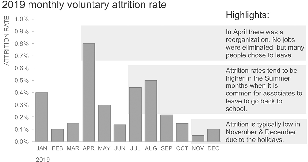
Figure 3.2e Enclosure
In Figure 3.2e, the light shading is meant to connect the data points to the text. If the data were shaped differently, this method may not work so well. For example, if the September bar had value 0.8%, this would be confusing because it would cross both the first and second grey shaded areas, and could cause us to think we should relate it to one of those, when really none of the text is about that particular data point.
Though I like how this looks, another drawback compared to the previous use of similarity of color is that we don’t have any visual cues to help us talk about this data. If I will be presenting this graph live, it can be useful to be able to say things like “Look at the red bar, which shows…” or “The blue bars indicate where…”. I could solve this by adding color to my shaded regions. See Figure 3.2f.

Figure 3.2f Enclosure with color differentiation
I could take this a step further and use similarity of color for sparing data and words in addition to the shaded regions to make it clear which text relates to which data points. See Figure 3.2g.

Figure 3.2g Enclosure plus similarity
Connection. Another way we could tie the words to the data is by physically connecting them. Figure 3.2h illustrates this.

Figure 3.2h Connection
This works well given the layout of the data and varying heights of bars. This method will look the cleanest when you have only a few lines and are able to orient them horizontally (diagonal lines look messy and are attention grabbing, so if you find yourself needing to use diagonal lines, I would recommend using similarity rather than connection). Notice that the lines themselves don’t need to draw any attention—they can be thin and light, so they are there for reference, but aren’t distracting from our data.
There is still some processing I have to do, though, with the view in Figure 3.2h. I have to read the middle block of text to know that it applies to not only the August bar, but also to the July bar that precedes it. Similar processing is needed for December and the final takeaway. I could ease this work by layering on similarity of color. See Figure 3.2i.

Figure 3.2i Connection plus similarity
Figure 3.2i makes it clear through both connection and similarity which text relates to which data.
In choosing among these options (and you may very well have come up with additional options), I tend to favor the simple similarity of color illustrated in Figure 3.2d. The preceding view in Figure 3.2i is a close second for me. How were the ideas you came up with similar or different from mine? After reading my explanation, does your decision about how you’d communicate this data stay the same?
As with most of what we’ve been discussing, there is no single right answer. Different people will make different choices. Of utmost importance is that you make it easy for your audience. When you show text and data together, make it clear to your audience when they read the text, where they should look in the data for evidence of what’s being said, and when they look at the data, where they should look in the text for additional detail. The Gestalt principles can help you achieve this.
Exercise 3.3: harness alignment & white space
We’ve looked at Gestalt principles for organizing what we see. We should also eliminate visual clutter. When elements aren’t aligned and white space is lacking, things feel cluttered. The concept is similar to cleaning up a messy room: put everything in its place and magic happens—the same items are present but now there is a harmonious sense of order.
Let’s do a quick exercise to illustrate how we can undertake a similar endeavor with our graphs. These seemingly minor components of our visual designs can have major impacts on the overall look and feel of what we create as well as the perceived ease with which our audience can consume it.
See Figure 3.3a, which is a slide showing data about physicians writing prescriptions (writers) for a pharmaceutical drug (Product X) across three different promotions (A, B, and C). The slopegraph compares the percent of total across the three promotion types between repeat writers (those physicians who have prescribed Product X before) at the left and new writers (those prescribing it for the first time) at the right. The details in this case aren’t so important. It’s probably also worthy of note that we could debate whether this is the best way to show this data, but let’s not worry about that—rather, let’s focus on how we might better arrange the current components.

Figure 3.3a How might we better use alignment & white space?
What changes would you make when it comes to alignment and white space to improve this visual? Are there other changes you would suggest? Write them down.
If you’d like, you can download this visual and implement the changes you’ve outlined.
Solution 3.3: harness alignment & white space
The visual in Figure 3.3a feels sloppy. It appears as if elements were simply thrown onto the slide. A couple of minutes and quick changes to alignment and use of white space can bring a sense of order and make the information easier to assimilate.
First, let’s discuss alignment. Currently, the text on the slide is all center-aligned. I tend to avoid center alignment because it can leave things hanging in space. Additionally, when the text flows onto multiple lines, it creates jagged edges that look messy. I’m an advocate of left or right-aligning text boxes to create clean vertical and horizontal lines across the elements. Doing so allows us to makes use of the Gestalt principle of closure—as we create framing, it helps tie the elements of the slide together. In this case, I’ll left-align the takeaways at the top, the graph title, and the left x-axis labels (Repeat writers, 92K). I’ll pull the data labels within the graph to be labeled at the left for Repeat writers and at the right for New writers. I’ll also pull the Promo A, Promo B, Promo C descriptions out of the middle of the graph and orient those on the right, lining them up horizontally with the data labels for those points (I could have also put these to the left of the left labels—which I choose typically depends where I want my audience to focus). Finally, I left-aligned the text at the right.
I left-justified most of the text (the only exception is the New writers and 45K x-axis label, which I’ve right-justified to provide framing on the right side of the graph). Which you choose between left or right alignment (or in rare instances, center alignment) depends on the layout of the elements on the rest of the page. The idea is to create clear vertical and horizontal lines. Sometimes right-justified text will also work well, and you’ll see this in a number of examples throughout this book. I did try right-aligning the text at the right side of the page, but it created some jagged trapped white space in the middle of the page that I didn’t like, so I reverted to left alignment.
The other change I made was in regards to white space. I pulled the graph title up so there would be a little space between it and the graph. I reduced the width of the graph both to allow room to label the various data series at the right as well as to have some space between that and the text box at the right. Probably the biggest (and fastest to implement) change in this area was simply adding line breaks to the text on the right, making it easier to scan and a little nicer to view.
You can see all of these changes implemented in Figure 3.3b.

Figure 3.3b Better employment of alignment & white space
Compare Figure 3.3b to Figure 3.3a. How does this ordered graph feel compared to the original? I appreciate the sense of structure in Figure 3.3b that was initially lacking.
You may have made some different decisions in your redesign, and that’s okay. The main point is to be thoughtful in your use of alignment and white space. These small things can have a big impact!
We’ll look at more examples illustrating the benefit of paying attention to detail in our visual design in Chapter 5.
Exercise 3.4: declutter!
A frequent source of clutter in data visualization comes from unnecessary graph elements: borders, gridlines, data markers, and the like. These can make our visuals appear overly complicated and increase the work our audience has to undertake in order to understand what they are viewing. As we eliminate the things that don’t need to be there, our data stands out more. Let’s take a closer look at the benefit that decluttering can have on our data visualizations.
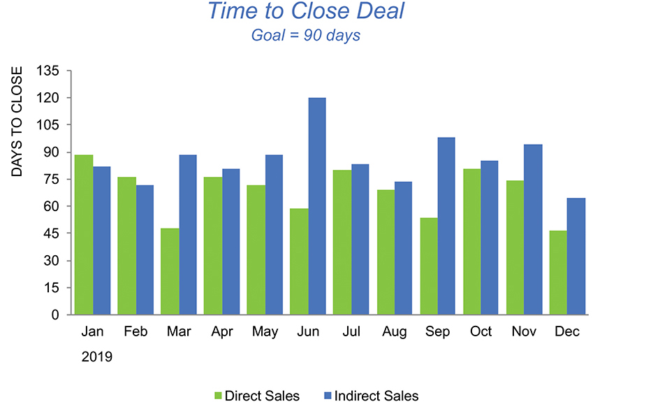
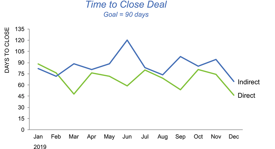
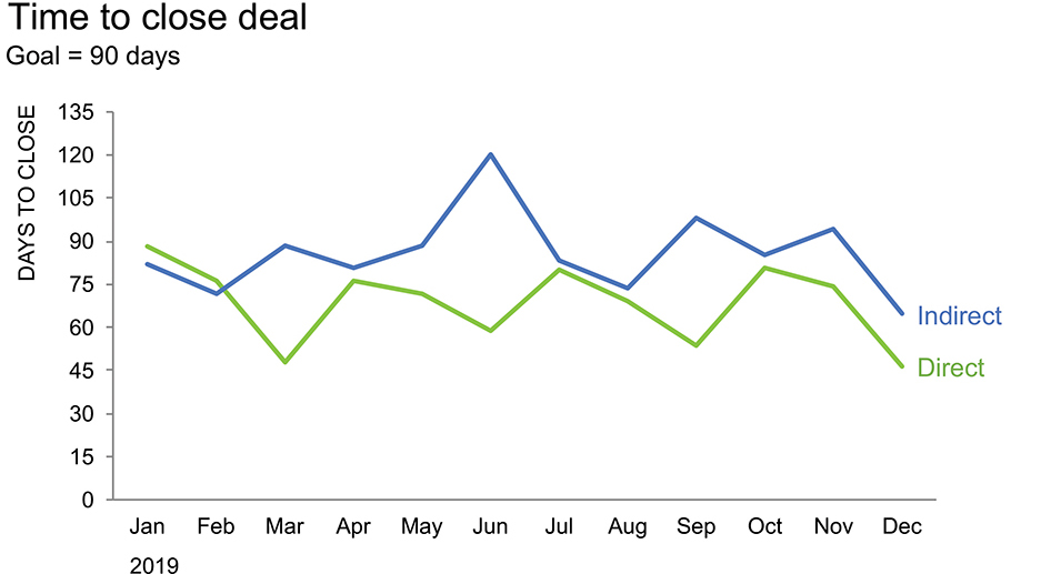
See Figure 3.4a, which shows time to close deals, measured in days, for direct and indirect sales teams over time.

Figure 3.4a Let’s declutter!
What visual elements could you eliminate? What other changes would you make to what is shown or how it’s shown to reduce cognitive burden? Spend a moment considering this and make some notes. How many changes would you make to this visual?
Solution 3.4: declutter!
I identified 15 changes I’d like to make to the Time to Close Deal graph. If your list falls short of this, refer back to Figure 3.4a and take another minute or two to see what else you might modify before you read through my ideas.
Ready? Let me walk you through what I would do—step by step—and my thought process behind each choice.
1. Remove heavy lines. The heavy horizontal lines between title and graph and at bottom graph border are unnecessary. The closure principle tells us we already see the graph as part of a whole—we don’t need these partial enclosures to make that clear. Use white space instead to set the title and graph apart from other elements as needed.

2. Remove gridlines. Gridlines are gratuitous! It’s amazing to me how much the simple steps of removing the chart border and gridlines do to make our data stand out more. See Figure 3.4c.

Figure 3.4c Remove gridlines
3. Drop trailing zeros from y-axis labels. This is one of my pet peeves! The zeros after the decimal place carry no information—get rid of them. I’m also going to change the frequency of my y-axis labels. While labeling every 20 makes sense given the scale of the numbers, we’re plotting days, so something like every 30 would make more sense (approximating a month). I started with that, but the axis looked overly sparse, so I opted for every 15 days. Let’s also add a y-axis title so we know what we’re looking at. I advocate titling axes directly so that your audience isn’t left questioning or having to make assumptions to decipher the data.

4. Eliminate diagonal text on x-axis. Diagonal text looks messy. Worse than that, studies have shown it’s slower to read than horizontal text (vertical text, by the way, is even slower). If efficiency of information transfer is one of your goals when communicating with data—which I’d argue it should be—aim for horizontal text whenever possible.
I see this issue often with diagonal x-axis labels, where the years are repeated with every date—which is both redundant and also space constraints frequently force the date to be diagonal. We can avoid this by using month abbreviations for the primary x-axis label, and then use year as supercategory x-axis label or title the axis with the year. In this case, I’ve simply titled the x-axis with the year (2019) to make the date range clear.

5. Thicken the bars! Another pet peeve is when the white space between the bars is bigger than the bars themselves. Let’s thicken those. This also makes use of the connection Gestalt principle, where with reduced distance between the bars, my eyes start to try to draw lines between the bars (if moving from bars to lines was on your list of recommendations, don’t worry, it’s on mine, too—we’ll get there soon!).

Figure 3.4f Thicken the bars!
6. Pull data labels into ends of bars. Now that we’ve thickened the bars, we have space to pull the data labels into the bars. This is a cognitive trick. Looking back to the previous iteration (Figure 3.4f), when we had a data label outside the end of each bar, each bar and label acted as two discrete elements. Now that we’ve thickened the bars, we can have room to embed the data labels, taking what were previously two distinct elements and turning them into a single element. This reduces the perceived cognitive burden, without reducing any of the actual data that we are showing.
Previously, we had a decimal of significance on each data label. This will always be context-dependent, but in this case given the scale of the numbers, we don’t need that specificity (also be cautious of the aforementioned false precision that having too many decimal places can convey). Here, we have an added benefit: reducing precision allows us to more cleanly fit the labels into the ends of the bars. I’ve made the labels white (versus the previous black), simply because I like the contrast you get with white-on-color. See Figure 3.4g.

Figure 3.4g Pull data labels into ends of bars
7. Eliminate data labels. In the previous step, I rounded and pulled the data labels into the ends of the bars. Note, though, that we don’t need both the y-axis and every data point labeled—this is redundant. This is a common decision point when it comes to visualizing data: do I preserve the axis, label the data directly, or some combination of the two? The main thing you want to consider when making this decision is the degree of importance of the specific numeric values. If it’s critical that your audience know that time to close a deal for Direct Sales went from exactly 74 days in November to exactly 46 days in December, then you could label the data directly and get rid of the y-axis altogether. If, on the other hand, you want your audience to focus on the shape of the data, or general trends or relationships, then I’d recommend preserving the axis and not cluttering the graph with the data labels.
In this case, I’ll assume the shape and general trends are more important than the precise numeric values. Because of this, I’m going to keep the y-axis and remove the data labels from each bar.
8. Make it a line graph. If you’ve been thinking this entire time: “This is data over time, so shouldn’t it be a line graph?” I’m with you. Check out the impact of moving from bars to lines. We’re using less ink, so the overall design feels cleaner. This is also a big win from a cognitive burden standpoint: we’ve taken what was previously twenty-four bars and replaced them with just two lines.

Figure 3.4i Make it a line graph
9. Label the data directly. Look back to Figure 3.4i and locate the legend. Your eyes do a bit of scanning to find it, right? This is work. It’s perhaps more noticeable now that we’ve taken a number of steps to reduce the other issues that were causing cognitive burden. This is the kind of work that we want to identify and take upon ourselves—as the designers of the information—so our audience doesn’t have to exert effort to figure out what they are seeing.
We can use the Gestalt principle of proximity to put the data labels right next to the data they describe. This eliminates any searching to figure out how to read the data.
10. Make data labels the same color as the data. While we leverage proximity—putting the data labels right next to the data they describe—let’s also make use of similarity, recoloring the data labels to match data they describe. It’s another visual cue to our audience to indicate that these things are related.

Figure 3.4k Make data labels the same color as the data
11. Upper-left-most orient graph title. Without other visual cues, your audience will start at the top left of your page, screen, or graph, and do zigzagging “z’s” to take in the information. Because of this, I advocate upper-left-most justifying graph and axis titles and labels. This means your audience sees how to read the data before they get to the data itself. As we discussed in Exercise 3.3, I tend to avoid center alignment of text because it leaves things hanging out in space (revisit Figure 3.4k and look at the graph title positioning). When you have text that goes onto multiple lines, this creates jagged edges that look messy. While I was changing the positioning of the title, I also eliminated the italics, which were unnecessary.

12. Remove title color. Up until now, the graph title has been blue. Did you find yourself trying to tie that to the Indirect trend in the data? That’s the Gestalt principle of similarity at play: we naturally try to associate things of similar color. In this case, that is a false association. Let’s eliminate it by taking color out of the title entirely (we’ll look at an alternative approach where we do use some color in the title to make use of this natural association momentarily).
13. Put the goal in the graph. Originally, the subtitle told us that the goal for time to close a deal is 90 days. If we want to be able to relate this to the data (are we above goal? below goal?)—which would make sense here—let’s put that information in the graph directly so we can visually compare the data and don’t have to really think about it.

14. Iterate to best visualize Goal. The Goal line is quite pronounced in the preceding graph. Let’s take a look at some different views. This is a good example of how allowing yourself time to iterate and look at things a number of different ways can be useful at many points during the process. I like using dotted lines for goals or targets, but when the line is thick, this introduces visual clutter. When I make the line thinner, it deemphasizes it—so it’s there and easy to see, but isn’t drawing undue attention. I also like all caps for short phrases, such as GOAL, because they are easy to scan and create nice rectangular shapes (versus mixed case, which doesn’t have clean lines at the top since letters such as l are taller than letters such as a).

Let’s look at a bigger version of that final iteration.

15. Remove color. Given that we have sufficient spatial separation between the lines in this graph, we don’t need to use color as a categorical differentiator the way we have up to this point. I’ll make everything grey. Color will come back into play when we focus attention—let’s do that next.

Focus attention. We’re jumping ahead, but now that we’ve come this far it only feels right that we carry this one through to the end. I’ll stop numbering my steps at this point, since I’m no longer decluttering. In the preceding view, I pushed everything to the background—made it all grey. This forces me to be thoughtful about where and how I direct my audience’s attention. There are a number of things we could point out in this data. Let’s assume for a moment that we want to draw attention to the Indirect data series in this graph.
Figure 3.4r illustrates one way I could achieve that.

Figure 3.4r Focus attention
Notice how my words above the graph are tied visually to the Indirect trend within the graph through similar use of color. This is akin to how we perhaps tried to tie the original blue title in the initial graph to the blue trend, only this time I’m doing it on purpose and it makes sense. By reading those words at the top of the graph, my audience will already know what to look for in the data before they get there. Also, if we think of this from a scannability standpoint, if I only look at this for a couple of seconds, the colored words and line draw my attention and I clearly and quickly get the takeaway that time to close indirect deals varies.
Focus attention elsewhere. I can use this same strategy and some highlighted data points to make a different point. See Figure 3.4s.

Figure 3.4s Focus attention elsewhere
Introduce a bit more color to really direct attention. I could take the preceding example a step further by introducing another color. I tend to avoid green for “good” and red for “bad,” because of the inaccessibility for colorblind audience members. Bright orange can have a similar negative connotation to red and stands out quite nicely given the other colors we have in play (this particular shade of blue was chosen because it matched the client’s branding).

Figure 3.4t Introduce a bit more color to really direct attention
Focus attention on yet another takeaway. If the times where we’ve missed goal aren’t the crux of the point we want to make, we could direct attention to a meta-takeaway: we’re beating our goal most of the time across both Indirect and Direct sales. We can use words and color to make this point clear. In this view, with the end markers and data labels, one obvious comparison for our audience to make is how Indirect and Direct time to close deals compared to each other and the goal in December.
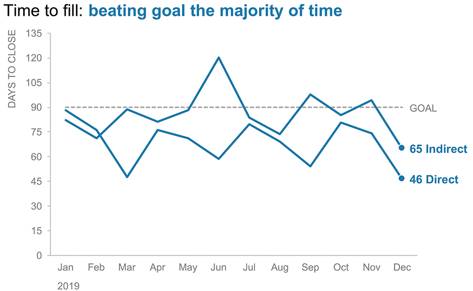
Figure 3.4u Focus attention on yet another takeaway
We’ll look at more strategies for focusing attention in Chapter 4.
Next, let’s shift gears and have you undertake some practice on your own.

Exercise 3.5: which Gestalt principles are in play?
As we’ve discussed and seen illustrated through a number of examples so far, Gestalt principles help us organize what we see, providing cues to what clutter we can eliminate and relating elements to each other in various ways. Consider the six principles we’ve covered—proximity, similarity, enclosure, closure, continuity, and connection—and review the following visual.
Which Gestalt principles are being used in Figure 3.5? Where and how? What effect does each achieve?

Figure 3.5 Which Gestalt principles are in play?
Exercise 3.6: find an effective visual
Find an example graph that you believe is effective. This can be from your work, someone else’s work, the media, storytellingwithdata.com, or other sources. Are any Gestalt principles being used? I’ll bet there are. Which and how? List them! What do the Gestalt principles you identify help achieve? What else do you like about the graph? What makes it effective?
Write a paragraph or two outlining your evaluation. See the following for reference.
Exercise 3.7: alignment & white space
Alignment and white space—these are elements of the visual design, that when done well, we don’t even notice. However when they aren’t done well, we feel it in the resulting visual. It may seem disorganized or connote lack of attention to detail, distracting from our data and message.
Consider Figure 3.7, which shows consumer sentiment based on survey results about various potential beverage line extensions for a food manufacturing company. Complete the following steps.

Figure 3.7 How can white space & alignment improve this visual?
STEP 1: Reflect on what specific changes you would recommend when it comes to the effective use of alignment and white space. List them.
STEP 2: Think back to the other lessons covered in this chapter (making use of Gestalt principles, decluttering, employing contrast). What other steps would you take to declutter or otherwise improve this visual?
STEP 3: Download the data and make the changes you’ve recommended to the existing graph, or import the data into your preferred tool and create a clutter-free visual that aligns elements and makes use of white space.
Exercise 3.8: declutter!
As we’ve seen through a number of the examples we’ve looked at already, there can be great value in identifying and removing things in our visuals that don’t need to be there. Each element we take away helps our data stand out more and frees up space so we can add things that matter. Let’s continue to practice this important skill of identifying clutter and removing it from our visual designs. We’ll do a few of these so you can have the opportunity to identify a number of different types of clutter.
Consider Figure 3.8, which shows customer satisfaction score over time. What unnecessary visual elements could you eliminate? What other changes would you make to reduce cognitive burden? Make some notes about the changes you would make to declutter this graph.

Figure 3.8 Let’s declutter!
To take it a step further, download the data and make the changes you’ve recommended to the existing graph, or import the data into your preferred tool and create a visual that is clutter-free.
Exercise 3.9: declutter (again!)
Clutter takes a lot of different forms. Let’s look at another example graph that can be improved.
Check out Figure 3.9, which shows the monthly number of cars sold by a national chain of dealerships. What unnecessary visual elements could you eliminate? What other changes would you make to reduce cognitive burden? Make some notes about the changes you would make to declutter this graph.

Figure 3.9 Let’s declutter!
To take it a step further, download the data and make the changes you’ve recommended to the existing graph, or import the data into your preferred tool and create a visual that is clutter-free.
Exercise 3.10: declutter (some more!)
Here is another opportunity to identify and eliminate clutter. See Figure 3.10, which shows the percent of customers of a given bank having automated payments by different products. What unnecessary visual elements could you eliminate? What other changes would you make to reduce cognitive burden? Make some notes about the changes you would make to declutter this graph.

Figure 3.10 Let’s declutter!
To take it a step further, download the data and make the changes you’ve recommended to the existing graph, or import the data into your preferred tool and create a visual that is clutter-free.

Exercise 3.11: start with a blank piece of paper
Often, the culprit behind the clutter in our visuals is our tool. When we draw, each stroke of the pen or pencil takes effort. We don’t tend to put forth that effort unless it’s worth it, which means it’s harder for non-information-carrying elements to work their way into our designs.
In the same way we used drawing to brainstorm and iterate through different views of our data in Chapter 2, there are benefits to drawing from a decluttering standpoint, too.
Consider a project where you need to communicate with data. Spend some time getting familiar with the data and what you want to communicate. Get yourself a blank piece of paper and sketch your visual. Consider whether you’ve included anything that’s not necessary. Once you have it right on paper, determine what tools or experts you have at your disposal to make your ideas real.
Exercise 3.12: do you need that?
Once we’ve taken the time to put something together, it can become difficult to look at it with fresh eyes and determine what we should eliminate. After creating a visual, pause and ask yourself the following questions. Or take an existing visual from a regular report or dashboard and assess how it could be improved through decluttering.
- What visual clutter can you eliminate? Are there any unnecessary elements distracting from your data or message? You can usually get rid of borders and gridlines. Is anything unnecessarily complicated? How might you simplify? What feels like work? How can you remedy? What other changes can you make to reduce cognitive burden?
- Is there redundant information you could streamline? It’s important to clearly title and label everything, but look for redundancy that can be eliminated. For example, decide whether an axis or data labels will best meet your needs—you typically won’t need both. Units should be clearly displayed, but may not need to be attached to every data point. Use effective titling to help streamline.
- Is all of the data you are showing necessary? Go through each piece of data in your graph or presentation and ask yourself whether you need it. If you plan to remove any data, consider what context you lose with it. In some cases, this still makes sense. As part of this, think about: what is the right time frame to show? What are the important comparison points? Are they all equally important? Reflect on what aggregation or frequency makes sense—sometimes rolling daily data into weekly or monthly data into quarterly (for example) can simplify and make it easier to see overarching trends.
- What could you push to the background? Not all elements in a chart or on a page are equally important. Where can you make use of grey to push non-message-impacting components to the background and employ strategic contrast to help direct attention?
- Seek feedback. Recruit a colleague to look at your visual and ask probing questions that will force you to talk through what you are showing. If you ever find yourself saying things like, “Ignore this” or they ask you questions about points that you thought were clear, these are verbal cues that you can use to further refine your visual, pushing less important elements to the background or getting rid of them entirely. Make changes and then go through the process with someone else. Iterate based on feedback to help push your work from good to great.
Exercise 3.13: let’s discuss
Consider the following questions related to Chapter 3 lessons and exercises. Discuss with a partner or group.
- Why is it important to identify and eliminate clutter? What are common types of clutter that you will remove from your visual communications going forward? When does it not make sense to spend time decluttering?
- Review the Gestalt principles. Which of these would you like to use more in your work? How will you do so? Are there any that don’t make sense or where you are unclear how you could use them in your work?
- Is there any common clutter that your graphing application routinely adds to your visuals? How can you streamline your process of decluttering to be more efficient in your tools?
- We’ve looked at some examples where data over time is plotted as bars. What are the benefits from a clutter standpoint of showing this data as a line graph? When would it make sense to do this? In what scenarios would you keep the bars?
- What is one tip you picked up from the lessons in this chapter that you plan to employ going forward? Where and how will you make use of it? Can you foresee exceptions where you wouldn’t put into practice the given strategy?
- Lining up elements, preserving white space, and employing strategic contrast: are these just about making things pretty, or is there more to it than that? Does this sort of attention to detail matter? Why or why not?
- Can you imagine any situations where clutter is desirable? When and why?
- What is one specific goal you will set for yourself or your team related to the strategies outlined in this chapter? How can you hold yourself (or your team) accountable to this? Who will you turn to for feedback?