CHAPTER
7

Probability and Counting Rules

In This Chapter

• Using the addition rule of probability
• Using the multiplication rule of probability
• Calculating conditional probabilities
• Using the Bayes’ theorem to calculate conditional probabilities
• Using the fundamental counting principle
• Distinguishing between permutations and combinations

Now that we have arrived at the second of three basic probability chapters, we’re ready for some new challenges. We need to take the probability concepts that you’ve mastered from Chapter 6 and put them to work on the next step up the ladder. Don’t worry if you’re afraid of heights like I am–just keep looking up!

This chapter deals with the topic of manipulating the probability of different events in various ways. As new information about events becomes available, we can revise the old information and make it more useful. This revised information can sometimes lead to surprising results–as you’ll soon see.

This chapter will also teach you how to count. This type of counting, however, goes far beyond what you’ve seen on Sesame Street. Counting events is an important step in calculating probabilities and must be done with care.

Addition Rule of Probabilities

In the previous chapter, we saw the union and intersection of events. Now we are going to put them to work. The addition rule of probability calculates the probability of the union of events–that is, the probability that either Event A or Event B will occur. For the addition rule, we need to distinguish between both mutually exclusive events and non-mutually exclusive events (we looked at mutually exclusive events in Chapter 6). The addition rule of probability states the following:

P(A or B) = P(A) + P(B)      If A and B are mutually exclusive events

P(A or B) = P(A) + P(B) – P(A and B)      If A and B are not mutually exclusive events

Now, let’s apply these two rules to examples so we can see the difference between them. In rolling a single die, what is the probability of getting a 3 or a 4?

First stop and ask yourself if you can get a 3 and a 4 at the same time when you roll a single die. If the answer is no, like in this example, then the events are mutually exclusive and you don’t need to include the third term of the equation. So the probability of rolling a 3 or a 4 is:

In another example, if you draw a card from a deck, what is the probability of getting a heart (H) or a jack (J)? P(H or J) = P(H) + P(J). Stop and ask yourself if you can draw a heart and a jack at the same time. If the answer is yes, like in this example, then the events are not mutually exclusive and you need to include the third term of the equation. There are four jacks in the deck of cards, and one of them is a heart, so this card has been counted twice: once as a jack (included in the four jacks) and once as a heart (included in the 13 hearts). Therefore we need to subtract it once to avoid double counting the card. The probability of getting a heart or a jack is:

To make sure we understand this rule, let’s apply it to one more example. The following contingency table represents the grade and the gender for 20 students in a statistics class.

If I want to know the probability that a randomly selected student in class has a grade in the 80s or 90s, I can use the addition rule: P(80s or 90s) = P(80s) + P(90s). I know I should not include the third term since these are mutually exclusive events. So the probability is:

If I want to know the probability that a randomly selected student in class is a male or has a grade in the 80s, I can use the addition rule again: P(M or 80s) = P(M) + P(80s). This time, I know I should also include the third term since these are not mutually exclusive events. So the probability is:

As you can see from the table, there are 3 students who are male with grades in the 80s. These 3 students are counted twice: once because they are male (included in the 10 males) and once because they have grades in the 80s (included in the 5 students with grades in the 80s). If I didn’t subtract these three students, then I would have double counted them.

Before we look at the multiplication rules of probability, we need to know another concept–conditional probability.

Conditional Probability

Conditional probability is the probability that Event A occurs given that (or on the condition that) Event B has already occurred. In other words, the probability of Event A is affected by the fact that Event B has already occurred. This means that the two events, A and B, are not independent of each other (Do you remember the independent events we talked about in the last chapter? It all comes back!). We use a different notation for conditional probability–the probability of A given B is written as P(A|B).

To demonstrate, in rolling a single die, what is the probability of getting a 4 given that it is an even number? Now see the difference in wording! If I say the probability of getting a 4 without any conditions, we know it is . However, I added a condition. (Let’s say I peeked and gave you the additional information that the number I rolled was an even number.) This condition limits your sample space to only 3 instead of 6. Therefore, P(4|Even) = = 0.3333.

Let’s look at another example to make sure we master the conditional probability concept. In drawing a card from a deck of cards, what is the probability that it is a jack given that it is a face card? Now we know the trick–I limited your sample space to the condition given, which is a face card. So the sample space is now 12. Then the probability of drawing a jack (J) given that it is a face (F) card is P(J|F) = = 0.3333.

As you might imagine, there is a formula to calculate the conditional probability:

P(A|B) =

Let’s apply this formula to our grade and gender example. If I want to know the probability that a randomly selected student has a grade in the 80s given that she is a female, I can plug it in as follows:

P(80s|F) = = = = 0.20

Now just for fun, I’ll introduce you to some more statistics jargon: prior probability and posterior probability. The probability of rolling a 4 without any condition is called a simple probability, or a prior probability, because it is derived only from the information currently available (that is, prior to receiving any conditional information). On the other hand, conditional probability is also known as posterior probability because it’s based on a revision of the prior probability, given additional information.

Conditional probability is very useful for determining the probability of compound events, as you will see in the following section.

Multiplication Rule of Probabilities

The multiplication rule of probability calculates the probability of the intersection of events, that is, the probability that both Event A and Event B will occur. The probability of Event A and Event B occurring at the same time is also called a joint probability. For the multiplication rule, we need to distinguish between independent and dependent events. The multiplication rule of probability states the following:

P(A and B) = P(A) × P(B)      If A and B are independent events

P(A and B) = P(A) × P(B|A)      If A and B are dependent events

To demonstrate using independent events, in flipping a coin two times, what is the probability of getting a head the first time (H₁) and a head the second time (H₂)? Since these are independent events, we use the following formula:

To demonstrate the multiplication rule with dependent events, let’s go back to our grade and gender example. If I want to know the probability that a randomly selected student is female (F) with a grade in the 80s, then we use the following formula:

When you have the data in a contingency table, it is easier to get the probability of F and 80s–just locate the number of females with grades in the 80s from the table (2), and then divide it by the total number of observations (20). Let’s prove the point by applying it to another example. What is the probability that a randomly selected student is male with a grade in the 90s? If you replied , then yes, you are correct. I agree, this method is way easier!

Since you now understand the probability rules of addition and multiplication, I’m going to introduce you next to the Bayes’ theorem, which is conditional probability in a more general format.

Bayes’ Theorem

Thomas Bayes (1701–1761) developed a mathematical rule that deals with calculating P(A|B) from the information about P(B|A). Bayes’ theorem states the following:

P(A|B) =

Where:

P(A’) = the probability of the complement of Event A

P(B|A’) = the probability of Event B, given that the complement to Event A has occurred.

Now that looks like a mouthful, but applying it to a new example will clear things up. In a different statistics class, 45 percent of students are male with a 75 percent probability of passing. The female students have an 80 percent probability of passing. If I randomly pick a student who is passing (PS), what is the probability that this student is female?

Students always say the most difficult part of Bayes’ theorem is all of the different parts, so let’s clear this up a little and break down the example. The pieces given in the example are:

P(M) = 0.45

P(PS|M) = 0.75

P(PS|F) = 0.8

You can easily figure that 55 percent of the students are female. So to calculate P(F|PS), we can apply Bayes’ theorem as follows:

Knowing that the student passed the exam, there is a 57 percent chance that the student is female. See, Bayes’ theorem is not so difficult after all!

You’ve learned the probability rules, so let’s move on to the last topic of this chapter, the counting principles.

Counting Principles

As we learned in the last chapter, to be able to use the classical probability approach, you need to know the total number of outcomes possible for the event of interest (the sample space). For simple events like rolling a die or drawing a card from a deck, it’s easy to count the number of outcomes in the sample space. But for other events like a state lottery drawing, finding the total number of outcomes is difficult. In these cases, counting rules come in handy to help us determine the number of possible outcomes of an experiment or event.

There are three main counting rules: the fundamental counting rule, permutations, and combinations. Let’s look at each.

The Fundamental Counting Rule

On a nice Sunday afternoon, your mom took you out for an ice cream. The ice cream shop has many choices, and you are standing there for some time trying to determine which to choose. There are eight flavors (vanilla, chocolate, mango, strawberry, peach, banana, raspberry, and coffee), two toppings (hot fudge and sprinkles), and three sizes (small, medium, and large). While you are looking at the assortment, you wonder how many different choices you have. The fundamental counting rule can help. This rule says that if one event (my flavor choice) can occur in m ways, and a second event (my topping choice) can occur in n ways, then the total number of possible ways that these two events can occur together is m × n ways. You can stretch this principle to more than two events.

If I extend this rule to all three choices I have in the ice cream shop, then to get the total number of choices I use multiplication: 8 flavors × 2 toppings × 3 sizes = 48 choices. When your mom says you are taking too long to decide, you tell her that you have 48 ice cream choices to choose from, and they’re summarized in the table below. Better make up your mind soon!

Another example of the fundamental counting rule is the number of automobile license plates that a state can issue. Pennsylvania license plates have three letters followed by four numbers. Your friend, who has not taken a statistics class yet, is telling you if the state eliminates the use of the letter O and the number 0 from license plates because they look alike, then the total number of possible license plates that Pennsylvania can issue will not decrease by much (because it’s only two figures). However, you have studied the counting rules and you know this is incorrect. To prove it to your friend, you showed him the total number of possible license plates Pennsylvania can issue in both cases as follows:

If all letters and numbers are allowed, using the fundamental counting rule, then the total number of possible license plate combinations is 26 × 26 × 26 × 10 × 10 × 10 × 10 = 175,760,000 combinations. If Pennsylvania eliminates the letter O and the number 0 to avoid confusion since they look alike, the total number of possible license plates is 25 × 25 × 25 × 9 × 9 × 9 × 9 = 102,515,625 choices. You proved your point to your friend and he was impressed by your knowledge, so he decided to take a statistics class next semester!

When you use the fundamental counting rule to determine the total number of possible outcomes, it’s important to know whether or not repetition is allowed. The previous rule assumes repetition is allowed, but if repetition is not allowed, then the number of ways in which each event can occur will decrease. Let’s see the difference between the two rules. In your summer job in a local grocery store, the manager asks you to design ID cards for employees. He wants each ID card to have four digits on it. He asks you how many ID cards he can make if repetition is allowed and if repetition is not allowed. You tell him that if repetition is allowed, then you can have 10,000 ID cards, but if repetition isn’t allowed, then you can only have 5,040 ID cards. You explain:

If repetition is allowed, then each digit on the ID card has 10 choices. So the first digit can be chosen out of 10 numbers, the second digit can be chosen out of 10 numbers, and so can the third and fourth digits. This gives us a total of 10 × 10 × 10 × 10 = 10,000 ID cards.

If repetition isn’t allowed (meaning the same number can’t be used more than once on each ID card), then the first digit on the ID card can be chosen out of 10 digits, but the second digit can only be chosen out of 9 digits—since one digit has already been chosen, it can’t be repeated. Then the third digit on the ID card can only be chosen out of 8 digits, and so on. Without repetition, the total number of ID cards we can make now is 10 × 9 × 8 × 7 = 5,040 ID cards.

The manager says he’s glad he asked you!

Permutations

Permutations are the number of different ways in which r objects can be chosen one at a time from n distinct objects, where the order is important. It can be found with _nP_r = .

For example, a TV director for the evening news wants to use 5 new stories to broadcast on the evening news. One story will be broadcast first, one will be second, one will be third, one will be fourth, and the last one will be the closing story. If the TV director has 10 new stories to choose from, in how many possible ways can the evening news show be set up?

Since the order of the stories is important, we use permutations. The number of possible ways the evening news show can be set up is

₁₀P₅ = = (10)(9)(8)(7)(6) = 30,240 different ways to set up the evening news show. I’m glad I’m not the TV evening news director!

Combinations

Combinations are similar to permutations except that the order of the objects is not important. The number of combinations in which r objects are selected from n possible objects can be found as follows:

_nC_r =

The number of combinations is always less than the number of permutations. In the combinations formula, dividing by r! removes the duplicates from the number of permutations. For each two letters, there are two permutations (since order is important, so AB is different from BA) but only one combination (since order is not important, so AB and BA are the same). Thus, dividing the permutation by r! eliminates the duplicates. To see that clearly, let’s look at the following example.

From the first 4 letters of the alphabet (A, B, C, and D), how many permutations of 2 letters can we get? How many combinations of 2 letters can we get?

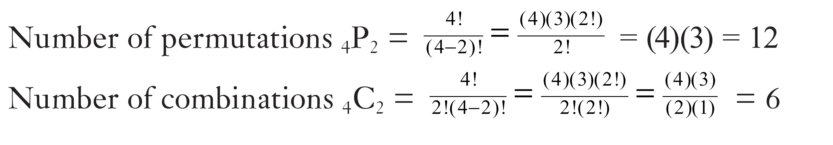
To see the difference, the permutations are:

Whereas the combinations are:

By eliminating the duplicates from the permutations, we get the combinations.

Combinations are often used in the selection of committees. As an example, your tennis club wants to choose an executive committee of 5 people. There are 12 people from whom to choose. How many different possibilities are there?

Number of combinations ₁₂C₅ = = 792 different ways to choose the committee.

Using Excel to Calculate Factorials, Permutations, and Combinations

Excel has built-in statistical functions that help us in all sorts of calculations, including factorials, permutations, and combinations. The Excel functions are:

Factorial = FACT(n)

Permutations = PERMUT(n,r)

Figure 7.2

Permutations function in Excel.

Combinations = COMBIN(n,r)

This concludes our discussion of probability and counting rules. Test your understanding by doing the practice problems.

Practice Problems

1. A political telephone survey asked 260 people whether they were in favor or not in favor of a proposed law. Each person was identified as a Republican or Democrat. The following contingency table shows the results.

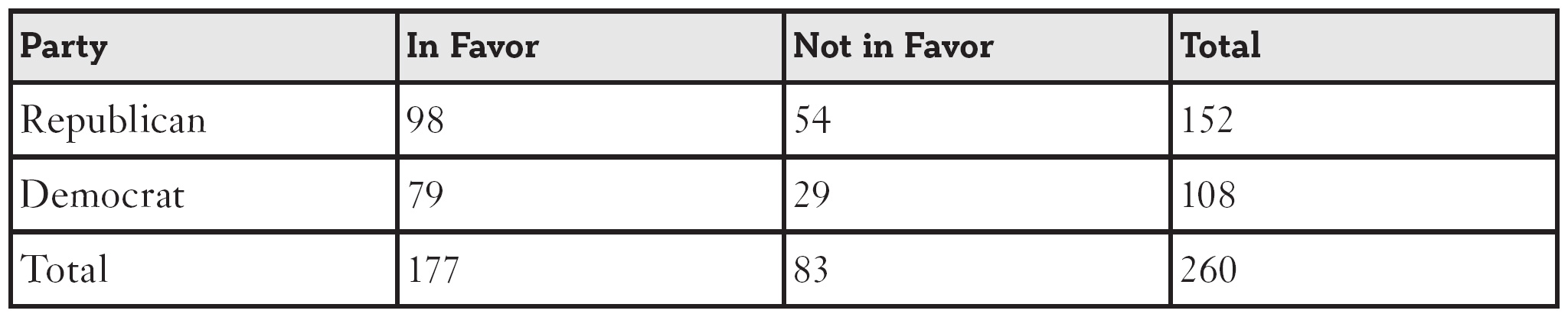
A person from the survey is selected at random. We define:

Event A: The person selected is in favor of the new law.

Event B: The person selected is a Republican.

a. Determine the probability that the selected person is in favor of the new law.

b. Determine the probability that the selected person is a Republican.

c. Determine the probability that the selected person is not in favor of the new law.

d. Determine the probability that the selected person is a Democrat.

e. Determine the probability that the selected person is in favor of the new law given that the person is a Republican.

f. Determine the probability that the selected person is not in favor of the new law given that the person is a Republican.

g. Determine the probability that the selected person is in favor of the new law given that the person is a Democrat.

h. Determine the probability that the selected person is in favor of the new law and that the person is a Republican.

i. Determine the probability that the selected person is in favor of the new law and that the person is a Democrat.

j. Determine the probability that the selected person is in favor of the new law or that the person is a Republican.

k. Determine the probability that the selected person is in favor of the new law or that the person is a Democrat.

l. Using Bayes’ theorem, calculate the probability that the selected person was a Republican, given that the person was in favor of the new law.

2. A survey asked 125 families whether the household had Internet access. Each family was classified by race. The following contingency table shows the results.

A family from the survey is randomly selected. We define:

Event A: The selected family has an Internet connection in its home.

Event B: The selected family is Asian American.

a. Determine the probability that the selected family has an Internet connection.

b. Determine the probability that the selected family is Asian American.

c. Determine the probability that the selected family has an Internet connection and is Asian American.

d. Determine the probability that the selected family has an Internet connection or is Asian American.

3. A restaurant has a menu with three appetizers, eight entrées, four desserts, and three drinks. How many different meals can you order?

4. A multiple-choice test has 10 questions, with each question having four choices. What is the probability that a student, who randomly answers each question, will answer each question correctly?

5. The NBA teams with the 13 worst records at the end of the season participate in a lottery to determine the order in which they will draft new players for the next season. How many different arrangements exist for the drafting order for these 13 teams?

6. In a race with eight swimmers, how many ways can swimmers finish first, second, and third?

7. How many different ways can 10 new movies be ranked first and second by a movie critic?

8. A combination lock has a total of 40 numbers and will unlock with the proper three-number sequence. How many possible combinations exist?

9. I would like to select three paperback books from a list of 12 books to take on vacation. How many different sets of three books can I choose?

10. A panel of 12 jurors needs to be selected from a group of 50 people. How many different juries can be selected?

The Least You Need to Know

• For mutually exclusive events, the addition rule states that P(A or B) = P(A) + P(B). If the events are not mutually exclusive, the addition rule becomes P(A or B) = P(A) + P(B) – P(A and B).
• We define conditional probability as the probability of Event A knowing that Event B has already occurred.
• For independent events, the multiplication rule states that P(A and B) = P(A) P(B). If the events are dependent, the multiplication rule becomes P(A and B) = P(A) P(B|A).
• Bayes’ theorem deals with calculating P(A|B) from information about P(B|A) using the following formula:
  
• The fundamental counting principle states that if one event can occur in m ways and a second event can occur in n ways, then the total number of ways both events can occur together is m · n ways. We can extend this principle to more than two events.
• Permutations are the number of different ways in which objects can be arranged in order. Combinations are the number of different ways in which objects can be arranged when order is of no importance.