Software Engineering for Embedded and Real-Time Systems
Rob Oshana Vice President of Software Engineering R&D, NXP Semiconductors, Austin, TX, United States
Abstract
Over the past 10 years or so, the world of computing has moved from large, static, desk-top machines to small, mobile, and embedded devices. The methods, techniques, and tools for developing software systems that were successfully applied in the former scenario are not as readily applicable in the latter. Software systems running on networks of mobile, embedded devices must exhibit properties that are not always required of more traditional systems.
Keywords
Software engineering; Software system; Embedded system; Real-time system; Hardware abstraction layers (HALs); Efficiency; Embedded software; Software driver
1 Software Engineering
Over the past 10 years or so, the world of computing has moved from large, static, desk-top machines to small, mobile, and embedded devices. The methods, techniques, and tools for developing software systems that were successfully applied in the former scenario are not as readily applicable in the latter. Software systems running on networks of mobile, embedded devices must exhibit properties that are not always required of more traditional systems:
- • Near-optimal performance
- • Robustness
- • Distribution
- • Dynamism
- • Mobility
This book will examine the key properties of software systems in the embedded, resource-constrained, mobile, and highly distributed world. We will assess the applicability of mainstream software engineering methods and techniques (e.g., software design, component-based development, software architecture, system integration, and testing) to this domain.
One of the differences in software engineering for embedded systems is the additional knowledge the engineer has of electrical power and electronics; physical interfacing of digital and analog electronics with the computer; and, software design for embedded systems and digital signal processors (DSPs).
Over 95% of software systems are embedded. Consider the devices you use at home daily:
- • Cell phone
- • iPod
- • Microwave
- • Satellite receiver
- • Cable box
- • Car motor controller
- • DVD player
So what do we mean by software engineering for embedded systems? Let’s look at this in the context of engineering in general. Engineering is defined as the application of scientific principles and methods to the construction of useful structures and machines. This includes disciplines such as:
- • Mechanical engineering
- • Civil engineering
- • Chemical engineering
- • Electrical engineering
- • Nuclear engineering
- • Aeronautical engineering
Software engineering is a term that is 35 years old, originating at a NATO conference in Garmisch, Germany, October 7–11, 1968. Computer science is its scientific basis with many aspects having been made systematic in software engineering:
- • Methods/methodologies/techniques
- • Languages
- • Tools
- • Processes
We will explore all these in this book.
The basic tenets of software engineering include:
- • Development of software systems whose size/complexity warrants team(s) of engineers (or as David Parnas puts it, “multi-person construction of multi-version software”).
- • Scope—we will focus on the study of software processes, development principles, techniques, and notations.
- • Goal, in our case the production of quality software, delivered on time, within budget, satisfying the customers’ requirements and the users’ needs.
With this comes the ever-present difficulties of software engineering that still exist today:
- • There are relatively few guiding scientific principles.
- • There are few universally applicable methods.
- • Software engineering is as much managerial/psychological/sociological as it is technological.
These difficulties exist because software engineering is a unique form of engineering:
- • Software is malleable
- • Software construction is human-intensive
- • Software is intangible
- • Software problems are unprecedentedly complex
- • Software directly depends upon the hardware
- • Software solutions require unusual rigor
- • Software has a discontinuous operational nature
Software engineering is not the same as software programming. Software programming usually involves a single developer developing “Toy” applications and involves a relatively short life span. With programming, there is usually a single stakeholder, or perhaps a few, and projects are mostly one-of-a-kind systems built from scratch with minimal maintenance.
Software engineering on the other hand involves teams of developers with multiple roles building complex systems with an indefinite life span. There are numerous stakeholders, families of systems, a heavy emphasis on reuse to amortize costs, and a maintenance phase that accounts for over 60% of the overall development costs.
There are both economic and management aspects of software engineering. Software production includes the development and maintenance (evolution) of the system. Maintenance costs represent most of all development costs. Quicker development is not always preferable. In other words, higher up-front costs may defray downstream costs. Poorly designed and implemented software is a critical cost factor. In this book we will focus on the software engineering of embedded systems, not the programming of embedded systems.
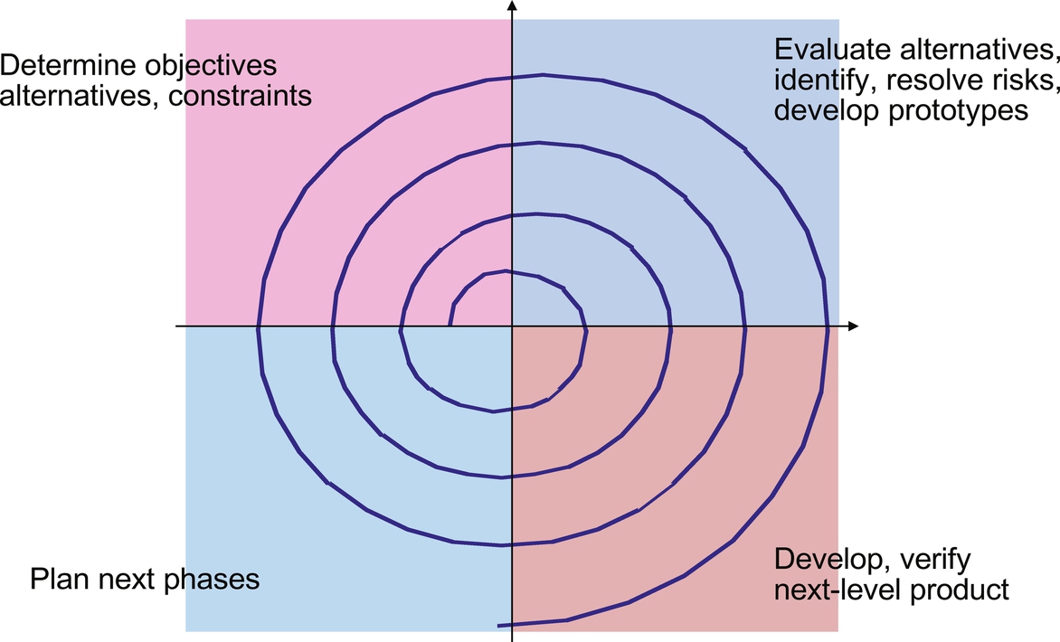
Embedded software development uses the same software development models as other forms of software development, including the Waterfall model (Fig. 1), the Spiral model (Fig. 2), and the Agile model (Fig. 3). The benefits and limitations of each of these models is well documented so we will only review them here. We will, however, spend more time later in this book on Agile development, as this approach is well suited to the changing, dynamic nature of embedded systems.


The key software development phases for embedded systems are briefly summarized below.
- 1. Problem definition. In this phase we determine exactly what the customer and user want. This may include the development of a contract with the customer, depending on what type of product is being developed. The goal of this phase is to specify what the software product is to do. Difficulties include the client asking for the wrong product, the client being computer/software illiterate which limits the effectiveness of this phase, and specifications that are ambiguous, inconsistent, and incomplete.
- 2. Architecture/design. Architecture is concerned with the selection of architectural elements, their interactions, and the constraints on those elements and their interactions necessary to provide a framework with which to satisfy the requirements and serve as a basis for the design. Design is concerned with the modularization and detailed interfaces of the design elements, their algorithms and procedures, and the data types needed to support the architecture and to satisfy the requirements. During the architecture and design phases, the system is decomposed into software modules with interfaces. During design the software team develops module specifications (algorithms, data types), maintains a record of design decisions and traceability, and specifies how the software product is to do its tasks. The primary difficulties during this phase include miscommunication between module designers and developing a design that may be inconsistent, incomplete, or ambiguous.
- 3. Implementation. During this phase the develop team implements the modules and components and verifies that they meet their specifications. Modules are combined according to the design. The implementation specifies how the software product does its task. Some of the key difficulties include module interaction errors and the order of integration that may influence quality and productivity.
More and more of the development of software for embedded systems is moving toward component-based development. This type of development is generally applicable for components of a reasonable size, reusing them across systems, something that is a growing trend in embedded systems. Developers ensure these components are adaptable to varying contexts and extend the idea beyond code to other development artifacts as well. This approach changes the equation from “Integration, Then Deployment” to “Deployment, Then Integration.”
There are different makes and models of software components:
- • Third-party software components
- • Plug-ins/add-ins
- • Frameworks
- • Open systems
- • Distributed object infrastructures
- • Compound documents
- • Legacy systems
- 4. Verification and validation (V&V). There are several forms of V&V and there is a dedicated chapter on this topic. One form is “analysis.” Analysis can be in the form of static, scientific, formal verification, and informal reviews and walkthroughs. Testing is a more dynamic form of V&V. This type of testing comes in the form of white box (having access to the code) and black box (having no access to the source code). Testing can be structural as well as behavioral. There are the standard issues of test adequacy but we will defer this discussion to later when we dedicate a chapter to this topic.
As we progress through this book, we will continue to focus on foundational software engineering principles (Fig. 4):
- • Rigor and formality
- • Separation of concerns
- – Modularity and decomposition
- – Abstraction
- • Anticipation of change
- • Generality
- • Incrementality
- • Scalability
- • Compositionality
- • Heterogeneity
- • Moving from principles to tools

2 Embedded Systems
What is an embedded system? There are many answers to this question. Some define an embedded system simply as “a computer whose end function is not to be a computer.” If we follow this definition then automobile antilock braking systems, digital cameras, household appliances, and televisions are embedded systems because they contain computers but aren’t intended to be computers. Conversely, the laptop computer I’m using to write this chapter is not an embedded system because it contains a computer that is intended to be a computer (see Bill Gatliff’s article “There’s no such thing as an Embedded System” on www.embedded.com).
Jack Ganssle and Mike Barr, in their book Embedded Systems Dictionary, define an embedded system as “A combination of computer hardware and software, and perhaps additional mechanical or other parts, designed to perform a dedicated function. In some cases, embedded systems are part of a larger system or product, as in the case of an antilock braking system in a car.”
Many definitions exist, but in this book we will proceed with the definition outlined in the following text.
An embedded system is a specialized computer system that is usually integrated as part of a larger system. An embedded system consists of a combination of hardware and software components to form a computational engine that will perform a specific function. Unlike desktop systems which are designed to perform a general function, embedded systems are constrained in their application.
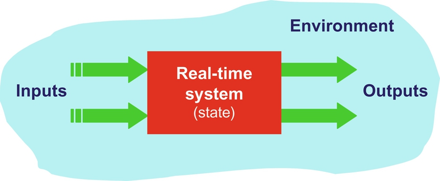
Embedded systems often perform in reactive and time-constrained environments. A rough partitioning of an embedded system consists of the hardware which provides the performance necessary for the application (and other system properties like security) and the software which provides most of the features and flexibility in the system. A typical embedded system is shown in Fig. 5.
- • Processor core. At the heart of the embedded system is the processor core(s). This can be a simple inexpensive 8-bit microcontroller or a more complex 32-bit or 64-bit microprocessor or can even be comprised of multiple processors. The embedded designer must select the most cost sensitive device for the application that can meet all the functional and nonfunctional (timing) requirements.
- • Analog I/O. D/A and A/D converters are used to get data from the environment and back out to the environment. The embedded designer must understand the type of data required from the environment, the accuracy requirements for that data, and the input/output data rates in order to select the right converters for the application. The external environment drives the reactive nature of the embedded system. Embedded systems must be at least fast enough to keep up with the environment. This is where the analog information, such as light or sound pressure or acceleration, is sensed and input into the embedded system.
- • Sensors and actuators. Sensors are used to sense analog information from the environment. Actuators are used to control the environment in some way.
- • User interfaces. These interfaces may be as simple as a flashing LED or as sophisticated as a cell phone or digital still camera interface.
- • Application specific gates. Hardware acceleration like ASIC or FPGA is used for accelerating specific functions in the application that have high-performance requirements. The embedded designer must be able to map or partition the application appropriately using the available accelerators to gain maximum application performance.
- • Software. Software is a significant part of embedded system development. Over the last few years the amount of embedded software has grown faster than Moore’s law, with the amount doubling approximately every 10 months. Embedded software is usually optimized in some way (performance, memory, or power). More and more embedded software is written in a high-level language like C/C ++ with some of the more performance-critical pieces of code still written in assembly language.
- • Memory is an important part of an embedded system and embedded applications can either run out of RAM or ROM depending on the application. There are many types of volatile and nonvolatile memory used for embedded systems and we will talk more about this later.
- • Emulation and diagnostics. Many embedded systems are hard to see or get to. There needs to be a way to interface to embedded systems to debug them. Diagnostic ports such as a JTAG (Joint Test Action Group) are used to debug embedded systems. On-chip emulation is used to provide visibility for the behavior of the application. These emulation modules provide sophisticated visibility for the runtime behavior and performance, in effect replacing external logic analyzer functions with onboard diagnostic capability.

2.1 Embedded Systems Are Reactive Systems
A typical embedded system responds to the environment via sensors and controls the environment using actuators (Fig. 6). This imposes a requirement on embedded systems to achieve performance consistent with that of the environment. This is why embedded system are often referred to as reactive systems. A reactive system must use a combination of hardware and software to respond to events in the environment within defined constraints. Complicating the matter is the fact that these external events can be periodic and predictable or aperiodic and hard to predict. When scheduling events for processing in an embedded system, both periodic and aperiodic events must be considered, and performance must be guaranteed for worst-case rates of execution.

An example of an embedded sensor system is a tire-pressure monitoring system (TPMS). This is a sensor chipset designed to enable a timely warning to the driver in the case of underinflated or overinflated tires on cars, trucks, or buses—even while in motion. These sensor systems are a full integration of a pressure sensor, an 8-bit microcontroller (MCU), a radio frequency (RF) transmitter, and X-axis and Z-axis accelerometers in one package. A key to this sensor technology is the acquisition of acceleration in the X and Z directions (Fig. 7). The purpose of X-axis and Z-axis g-cells are to allow tire recognition with the appropriate embedded algorithms analyzing the rotating signal caused by the Earth’s gravitational field. Motion will use either the Z-axis g-cell to detect acceleration level or the X-axis g-cell to detect a ± 1-g signal caused by the Earth’s gravitational field.

There are several key characteristics of embedded systems:
- (a) Monitoring and reacting to the environment. Embedded systems typically get input by reading data from input sensors. There are many different types of sensors that monitor various analog signals in the environment including temperature, sound pressure, and vibration. This data is processed using embedded system algorithms. The results may be displayed in some format to a user or simply used to control actuators (like deploying the airbags and calling the police).
- (b) Control the environment. Embedded systems may generate and transmit commands that control actuators, such as airbags, motors, etc.
- (c) Processing information. Embedded systems process the data collected from the sensors in some meaningful way, such as data compression/decompression, side impact detection, etc.
- (d) Application specific. Embedded systems are often designed for applications, such as airbag deployment, digital still cameras, or cell phones. Embedded systems may also be designed for processing control laws, finite-state machines, and signal-processing algorithms. Embedded systems must also be able to detect and react appropriately to faults in both the internal computing environment as well as the surrounding systems.
- (e) Optimized for the application. Embedded systems are all about performing the desired computations with as few resources as possible in order to reduce cost, power, size, etc. This means that embedded systems need to be optimized for the application. This requires software as well as hardware optimization. Hardware needs to be able to perform operations in as few gates as possible, and software must be optimized to perform operations in the least number of cycles, amount of memory, or power as possible depending on the application.
- (f) Resource constrained. Embedded systems are optimized for the application which means that many of the precious resources of an embedded system, such as processor cycles, memory, and power, are in scarce supply in a relative sense in order to reduce cost, size, weight, etc.
- (g) Real time. Embedded systems must react to the real-time changing nature of the environment in which they operate. More on real-time systems below.
- (h) Multirate. Embedded systems must be able to handle multiple rates of processing requirements simultaneously, for example video processing at 30 frames per second (30 Hz) and audio processing at 20-kHz rates.
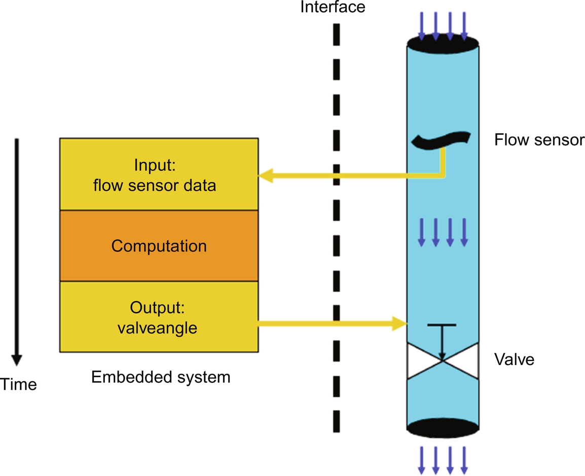
Fig. 8 shows a simple embedded system that demonstrates these key characteristics:
- 1. Monitoring and controlling the environment. The embedded system monitors a fluid-flow sensor in the environment and then controls the value (actuator) in that same environment.
- 2. Performing meaningful operations. The computation task computes the desired algorithms to control the value in a safe way.
- 3. Application specific. The embedded system is designed for a particular application.
- 4. Optimized for application. The embedded system’s computation and algorithms are designed for a particular system.
- 5. Resource constrained. The embedded system executes on a small inexpensive microcontroller with a small amount of memory, operating at lower power for cost savings.
- 6. Real time. The system has to be able to respond to the flow sensor in real time, any delays in processing could lead to failure of the system.
- 7. Multirate. There may be the need to respond to the flow sensor as well as a user interface, so multiinput rates to the embedded system should be possible.
3 Real-Time Systems
A real-time system is any information-processing activity or system which must respond to externally generated input stimuli within a finite and specified period. Real-time systems must process information and produce a response within a specified time. Failure to do so will risk severe consequences, including failure. In a system with a real-time constraint, it is unacceptable to have the correct action or the correct answer after a certain deadline: the result must be produced by the deadline or the system will degrade or fail completely. Generally, real-time systems maintain a continuous, timely interaction with the environment (Fig. 9).
3.1 Types of Real-Time Systems—Soft and Hard
In real-time systems, the correctness of the computation depends not only upon its results but also the time at which its outputs are generated. A real-time system must satisfy response time constraints or suffer significant system consequences. If the consequences consist of a degradation of performance, but not failure, the system is referred to as a soft real-time system. If the consequences are system failure, the system is referred to as a hard real-time system (e.g., an antilock braking system in an automobile) (Fig. 10).

We can also think of this in terms of the real-time interval, which is defined as how quickly the system must respond. In this context, the Windows operating system is soft real-time because it is relatively slow and cannot handle shorter time constraints. In this case, the system does not “fail” but is degraded.
The objective of an embedded system is to execute as fast as necessary in an asynchronous world using the smallest amount of code with the highest level of predictability. (Note: predictability is the embedded world’s term for reliability.)
Fig. 11 shows some examples of hard and soft real-time systems. As shown in this list of examples, many embedded systems also have a criticality to the computation in the sense that a failure to meet real-time deadlines can have disastrous consequences. For example, the real-time determination of a driver’s intentions and driving conditions (Fig. 12) is an example of a hard real-time safety critical application.


3.2 Differences Between Real-Time and Time-Shared Systems
Real-time systems are different from time-shared systems in three fundamental areas (Table 1):
- • High degree of schedulability. Timing requirements of the system must be satisfied at high degrees of resource usage and offer predictably fast responses to urgent events.
- • Worst case latency. Ensuring the system still operates under worst-case response times to events.
- • Stability under transient overload. When the system is overloaded by events and it is impossible to meet all deadlines, the deadlines of selected critical tasks must still be guaranteed.
Table 1
| Characteristic | Time-Shared Systems | Real-Time Systems |
|---|---|---|
| System capacity | High throughput | Schedulability and the ability of system tasks to meet all deadlines |
| Responsiveness | Fast average response time | Ensured worst-case latency which is the worst-case response time to events |
| Overload | Fairness to all | Stability; when the system is overloaded important tasks must meet deadlines while others may be starved |
4 Example of a Hard Real-Time System
Many embedded systems are real-time systems. As an example, assume that an analog signal is to be processed digitally. The first question to consider is how often to sample or measure the analog signal in order to represent that signal accurately in the digital domain. The sample rate is the number of samples of an analog event (like sound) that are taken each second to represent the event in the digital domain. Based on a signal processing rule called Nyquist, the signal must be sampled at a rate at least equal to twice the highest frequency that we wish to preserve. For example, if the signal contains important components at 4 kHz, then the sampling frequency would need to be at least 8 kHz. The sampling period would then be:
4.1 Based on Signal Sample, Time to Perform Actions Before Next Sample Arrives
This tells us that, for this signal being sampled at this rate, we would have 0.000125 s to perform all the processing necessary before the next sample arrived. Samples are arriving on a continuous basis and if the system falls behind in processing these samples, the system will degrade. This is an example of a soft real-time embedded system.
4.2 Hard Real-Time Systems
The collective timeliness of the hard real-time tasks is binary—i.e., either they all will always meet their deadlines (in a correctly functioning system) or they will not (the system is infeasible). In all hard real-time systems, collective timeliness is deterministic. This determinism does not imply that the actual individual task completion times, or the task execution ordering, are necessarily known in advance.
A computing system being a hard real-time system says nothing about the magnitudes of the deadlines. They may be microseconds or weeks. There is a bit of confusion with regards to the usage of the term “hard real-time.” Some relate hard real-time to response time magnitudes below some arbitrary threshold, such as 1 ms. This is not the case. Many of these systems actually happen to be soft real-time systems. These systems would be more accurately termed “real fast” or perhaps “real predictable.” But certainly not hard real-time systems.
The feasibility and costs (e.g., in terms of system resources) of hard real-time computing depend on how well known á priori are the relevant future behavioral characteristics of the tasks and execution environment. These task characteristics include:
- • Timeliness parameters, such as arrival periods or upper bounds
- • Deadlines
- • Worst-case execution times
- • Ready and suspension times
- • Resource utilization profiles
- • Precedence and exclusion constraints
- • Relative importance, etc.
There are also important characteristics relating to the system itself, including:
- • System loading
- • Resource interactions
- • Queuing disciplines
- • Arbitration mechanisms
- • Service latencies
- • Interrupt priorities and timing
- • Caching
Deterministic collective task timeliness in hard (and soft) real-time computing requires that the future characteristics of the relevant tasks and execution environment be deterministic—i.e., known absolutely in advance. Knowledge of these characteristics must then be used to preallocate resources so that hard deadlines, like motor control, will be met and soft deadlines, like responding to a key press, can be delayed.
A real-time system task and execution environment must be adjusted to enable a schedule and resource allocation which meets all deadlines. Different algorithms or schedules which meet all deadlines are evaluated with respect to other factors. In many real-time computing applications getting the job done at the lowest cost is usually more important than simply maximizing the processor utilization (if this was true, we would all still be writing assembly language). Time to market, for example, may be more important than maximizing utilization due to the cost of squeezing the last 5% of efficiency out of a processor.
Allocation for hard real-time computing has been performed using various techniques. Some of these techniques involve conducting an offline enumerative search for a static schedule which will deterministically always meet all deadlines. Scheduling algorithms include the use of priorities that are assigned to the various system tasks. These priorities can be assigned either offline by application programmers or online by the application or operating system software. The task priority assignments may either be static (fixed), as with rate monotonic algorithms or dynamic (changeable), as with the earliest deadline first algorithm.
5 Real-Time Event Characteristics
5.1 Real-Time Event Categories
Real-time events fall into one of three categories: asynchronous, synchronous, or isochronous:
- • Asynchronous events are entirely unpredictable. An example of this is a cell phone call arriving at a cellular base station. As far as the base station is concerned, the action of making a phone call cannot be predicted.
- • Synchronous events are predictable events and occur with precise regularity. For example, the audio and video in a camcorder take place in synchronous fashion.
- • Isochronous events occur with regularity within a given window of time. For example, audio data in a networked multimedia application must appear within a window of time when the corresponding video stream arrives. Isochronous is a subclass of asynchronous.
In many real-time systems, task and execution environment characteristics may be hard to predict. This makes true, hard real-time scheduling infeasible. In hard real-time computing, deterministic satisfaction of the collective timeliness criterion is the driving requirement. The necessary approach to meeting that requirement is static (i.e., á priori) scheduling of deterministic tasks and execution environment characteristic cases. The requirement for advanced knowledge about each of the system tasks and their future execution environment to enable offline scheduling and resource allocation significantly restricts the applicability of hard real-time computing.
5.2 Efficient Execution and the Execution Environment
5.2.1 Efficiency Overview
Real-time systems are time critical and the efficiency of their implementation is more important than in other systems. Efficiency can be categorized in terms of processor cycles, memory, or power. This constraint may drive everything from the choice of processor to the choice of programming language. One of the main benefits of using a higher level language is to allow the programmer to abstract away implementation details and concentrate on solving the problem. This is not always true in the world of the embedded system. Some higher level languages have instructions that are an order of magnitude slower than assembly language. However, higher level languages can be used in real-time systems effectively using the right techniques. We will be discussing much more about this topic in the chapter on optimizing source code for DSPs.
5.2.2 Resource Management
A system operates in real time as long as it completes its time-critical processes with acceptable timeliness. “Acceptable timeliness” is defined as part of the behavioral or “nonfunctional” requirements for the system. These requirements must be objectively quantifiable and measureable (stating that the system must be “fast,” for example, is not quantifiable). A system is said to be a real-time system if it contains some model of real-time resource management (these resources must be explicitly managed for the purpose of operating in real time). As mentioned earlier, resource management may be performed statically offline or dynamically online.
Real-time resource management comes at a cost. The degree to which a system is required to operate in real time cannot necessarily be attained solely by hardware overcapacity (e.g., high processor performance using a faster CPU).
There must exist some form of real-time resource management to be cost effective. Systems which must operate in real time consist of both real-time resource management and hardware resource capacity. Systems which have interactions with physical devices may require higher degrees of real-time resource management. One resource management approach that is used is static and requires analysis of the system prior to it executing in its environment. In a real-time system, physical time (as opposed to logical time) is necessary for real-time resource management in order to relate events to the precise moments of occurrence. Physical time is also important for action time constraints as well as measuring costs incurred as processes progress to completion. Physical time can also be used for logging history data.
All real-time systems make trade-offs of scheduling costs versus performance in order to reach an appropriate balance for attaining acceptable timeliness between the real-time portion of the scheduling optimization rules and the offline scheduling performance evaluation and analysis.
6 Challenges in Real-Time System Design
Designing real-time systems poses significant challenges to the designer. One of the significant challenges comes from the fact that real-time systems must interact with the environment. The environment is complex and changing and these interactions can become very complex. Many real-time systems don’t just interact with one entity but instead interact with many different entities in the environment, with different characteristics and rates of interaction. A cell phone base station, for example, must be able to handle calls from literally thousands of cell phone subscribers at the same time. Each call may have different requirements for processing as well as different sequences of processing. All this complexity must be managed and coordinated.
6.1 Response Time
Real-time systems must respond to external interactions in the environment within a predetermined amount of time. Real-time systems must produce the correct result and produce it in a timely way. The response time is as important as producing correct results. Real-time systems must be engineered to meet these response times. Hardware and software must be designed to support response time requirements for these systems. Optimal partitioning of system requirements into hardware and software is also important.
Real-time systems must be architected to meet system response time requirements. Using combinations of hardware and software components, it is engineering that makes the architecture decisions, such as interconnectivity of system processors, system link speeds, processor speeds, memory size, I/O bandwidth, etc. Key questions to be answered include:
- • Is the architecture suitable? To meet system response time requirements, the system can be architected using one powerful processor or several smaller processors. Can the application be partitioned among the several smaller processors without imposing large communication bottlenecks throughout the system? If the designer decides to use one powerful processor, will the system meet its power requirements? Sometimes a simpler architecture may be the better approach—more complexity can lead to unnecessary bottlenecks which cause response time issues.
- • Are the processing elements powerful enough? A processing element with high utilization (greater than 90%) will lead to unpredictable runtime behavior. At this utilization level lower priority tasks in the system may be starved. As a general rule, real-time systems that are loaded at 90% take approximately twice as long to develop due to cycles of optimization and integration issues with the system at these utilization rates. At 95% utilization, systems can take three times longer to develop due to these same issues. Using multiple processors will help but interprocessor communication must be managed.
- • Are the communication speeds adequate? Communication and I/O is a common bottleneck in real-time embedded systems. Many response time problems come not from the processor being overloaded but in latencies in getting data into and out of the system. In other cases, overloading a communication port (greater than 75%) can cause unnecessary queuing in different system nodes, causing delays in message passing throughout the rest of the system.
- • Is the right scheduling system available? In real-time systems tasks that are processing real-time events must take higher priority. But how do you schedule multiple tasks that are all processing real-time events. There are several scheduling approaches available and the engineer must design the scheduling algorithm to accommodate system priorities in order to meet all real-time deadlines. Because external events may occur at any time, the scheduling system must be able to preempt currently running tasks to allow higher priority tasks to run. The scheduling system (or real-time operating system) must not introduce a significant amount of overhead into the real-time system.
6.2 Recovering From Failures
Real-time systems interact with the environment, which is inherently unreliable. Therefore real-time systems must be able to detect and overcome failures in the environment. In addition, since real-time systems are also embedded into other systems and may be hard to get at (such as a spacecraft or satellite) these systems must also be able to detect and overcome internal failures as well (there is no “reset” button in easy reach of the user!). Also, since events in the environment are unpredictable, it is almost impossible to test for every possible combination and sequence of events in the environment. This is a characteristic of real-time software that makes it somewhat nondeterministic in the sense that it is almost impossible in some real-time systems to predict the multiple paths of execution based on the nondeterministic behavior of the environment. Examples of internal and external failures that must be detected and managed by real-time systems include:
- • Processor failures
- • Board failures
- • Link failures
- • Invalid behavior of the external environment
- • Interconnectivity failure
Many real-time systems are embedded systems with multiple inputs and outputs and multiple events occurring independently. Separating these tasks simplifies programming but requires switching back and forth among the multiple tasks. This is referred to as multitasking. Concurrency in embedded systems is the appearance of multiple tasks executing simultaneously. For example, the three tasks listed in Fig. 13 will execute on a single embedded processor and the scheduling algorithm is responsible for defining the priority of execution of these three tasks.

7 The Embedded System’s Software Build Process
Another difference in embedded systems is the software system build process, as shown in Fig. 14.

Embedded system programming is not substantially different from ordinary programming. The main difference is that each target hardware platform is unique. The process of converting the source code representation of embedded software into an executable binary image involves several distinct steps:
- • Compiling/assembling using an optimizing compiler.
- • Linking using a linker.
- • Relocating using a locator.
In the first step, each of the source files must be compiled or assembled into object code. The job of a compiler is mainly to translate programs written in some human readable format into an equivalent set of opcodes for a particular processor. The use of the cross compiler is one of the defining features of embedded software development.
In the second step, all the object files that result from the first step must be linked together to produce a single object file, called the relocatable program. Finally, physical memory addresses must be assigned to the relative offsets within the relocatable program in a process called relocation. The tool that performs the conversion from relocatable to executable binary image is called a locator. The result of the final step of the build process is an absolute binary image that can be directly programmed into a ROM or flash device.
We have covered several areas where embedded systems differ from other desktop-like systems. Some other differences that make embedded systems unique include:
- 1. Energy efficiency (embedded systems, in general, consume the minimum power for their purpose).
- 2. Custom voltage/power requirements.
- 3. Security (need to be hacker proof, for example, a Femto basestation needs IP security when sending phone calls over an internet backhaul).
- 4. Reliability (embedded systems need to work without failure for days, months, and years).
- 5. Environment (embedded systems need to operate within a broad temperature range, be sealed from chemicals, and be radiation tolerant).
- 6. Efficient interaction with user (fewer buttons, touchscreen, etc.).
- 7. Designed in parallel with embedded hardware.
The chapters in this book will touch on many of these topics as they relate to software engineering for embedded systems.
8 Distributed and Multiprocessor Architectures
Some real-time systems are becoming so complex that applications are executed on multiprocessor systems that are distributed across some communication system. This poses challenges to the designer that relate to the partitioning of the application in a multiprocessor system. These systems will involve processing on several different nodes. One node may be a DSP, another a more general-purpose processor, some specialized hardware processing elements, etc. This leads to several design challenges for the engineering team:
- • Initialization of the system. Initializing a multiprocessor system can be complicated. In most multiprocessor systems the software load file resides on the general-purpose processing node. Nodes that are directly connected to the general-purpose processor, for example, a DSP, will initialize first. After these nodes complete loading and initialization, other nodes connected to it may then go through this same process until the system completes initialization.
- • Processor interfaces. When multiple processors must communicate with each other, care must be taken to ensure that messages sent along interfaces between the processors are well-defined and consistent with the processing elements. Differences in message protocol including endianness, byte ordering, and other padding rules can complicate system integration, especially if there is a system requirement for backwards compatibility.
- • Load distribution. As mentioned earlier, multiple processors lead to the challenge of distributing the application and possibly developing the application to support an efficient partitioning of the application among the processing elements. Mistakes in partitioning the application can lead to bottlenecks in the system and this degrades the full entitlement of the system by overloading certain processing elements and leaving others underutilized. Application developers must design an application to be efficiently partitioned across processing elements.
- • Centralized resource allocation and management. In a system of multiple processing elements, there is still a common set of resources including peripherals, crossbar switches, memory, etc., that must be managed. In some cases the operating system can provide mechanisms like semaphores to manage these shared resources. In other cases there may be dedicated hardware to manage the resources. Either way, important shared resources in the system must be managed in order to prevent further system bottlenecks.
9 Software for Embedded Systems
This book will spend a considerable amount of time covering each phase of software development for embedded systems. Software for embedded systems is also unique from other “run to completion” or other desktop software applications. So we will introduce the concepts here and go into more detail in later chapters.
9.1 Super Loop Architecture
The most straightforward software architecture for embedded systems is the “super loop architecture.” This approach is used because when programming embedded systems it is very important to meet the deadlines of the system and to complete all the key tasks of the system in a reasonable amount of time, and in the right order. Super loop architecture is a common program architecture that is very useful in fulfilling these requirements. This approach is a program structure comprised of an infinite loop, with all the tasks of the system contained in that loop structure. An example is shown in Fig. 15.

The initialization routines are completed before entering the super loop because the system only needs to be initialized once. Once the infinite loop begins, the valves are not reset because of the need to maintain a persistent state in the embedded system.
The loop is a variant of the “batch processing” control flow: read input, calculate some values, write out values. Embedded systems software is not the only type of software which uses this kind of architecture. Computer games often use a similar loop called the (tight) (main) game loop. The steps that are followed in this type of gaming technology are:
- Function Main_Game_Function()
- {
- Initialization();
- Do_Forever
- {
- Game_AI();
- Move_Objects();
- Scoring();
- Draw_Objects();
- }
- Cleanup();
- }
9.2 Power-Saving Super Loop
The super loop discussed previously works fine unless the scheduling requirements are not consistent with the loop execution time. For example, assume an embedded system with an average loop time of 1 ms that needs to check a certain input only once per second. Does it really make sense to continue looping the program every 1 ms? If we let the loop continue to execute, the program will loop 1000 times before it needs to read the input again. Therefore, 999 loops of the program will effectively countdown to the next read. In situations like this an expanded super loop can be used to build in a delay as shown in Fig. 16.

Let’s consider a microcontroller that uses 20 mA of current in “normal mode” but only needs 5 mA of power in “low-power mode.” Assume using the super loop example outlined in the earlier text, which is in “low-power mode” 99.9% of the time (a 1-ms calculation every second) and is only in normal mode 0.1% of the time. An example of this is an LCD communication protocol used in alphanumeric LCD modules. The components provides methods to wait for a specified time. The foundation to wait for a given time is to wait for a number of CPU or bus cycles. As a result, the component implements the two methods: Wait10Cycles() and Wait100Cycles(). Both are implemented in assembly code as they are heavily CPU dependant.
9.3 Window Lift Embedded Design
Let’s look at an example of a slightly more advanced software architecture. Fig. 17 shows a simplified diagram of a window lift. In some countries it is a requirement to have mechanisms to detect fingers in window areas to prevent injury. In some cases, window cranks are now outlawed for this reason. Adding a capability like this after the system has already been deployed could result in difficult changes to the software. The two options would be to add this event and task to the control loop or add a task.

When embedded software systems become complex, we need to move away from simple looping structures and migrate to more complex tasking models. Fig. 18 is an example of what a tasking model would look like for the window lift example. As a general guideline, when the control loop gets ugly then go to multitasking and when you have too many tasks go to Linux, Windows, or some other similar type of operating system. We’ll cover all these alternatives in more detail in later chapters.

10 Hardware Abstraction Layers for Embedded Systems
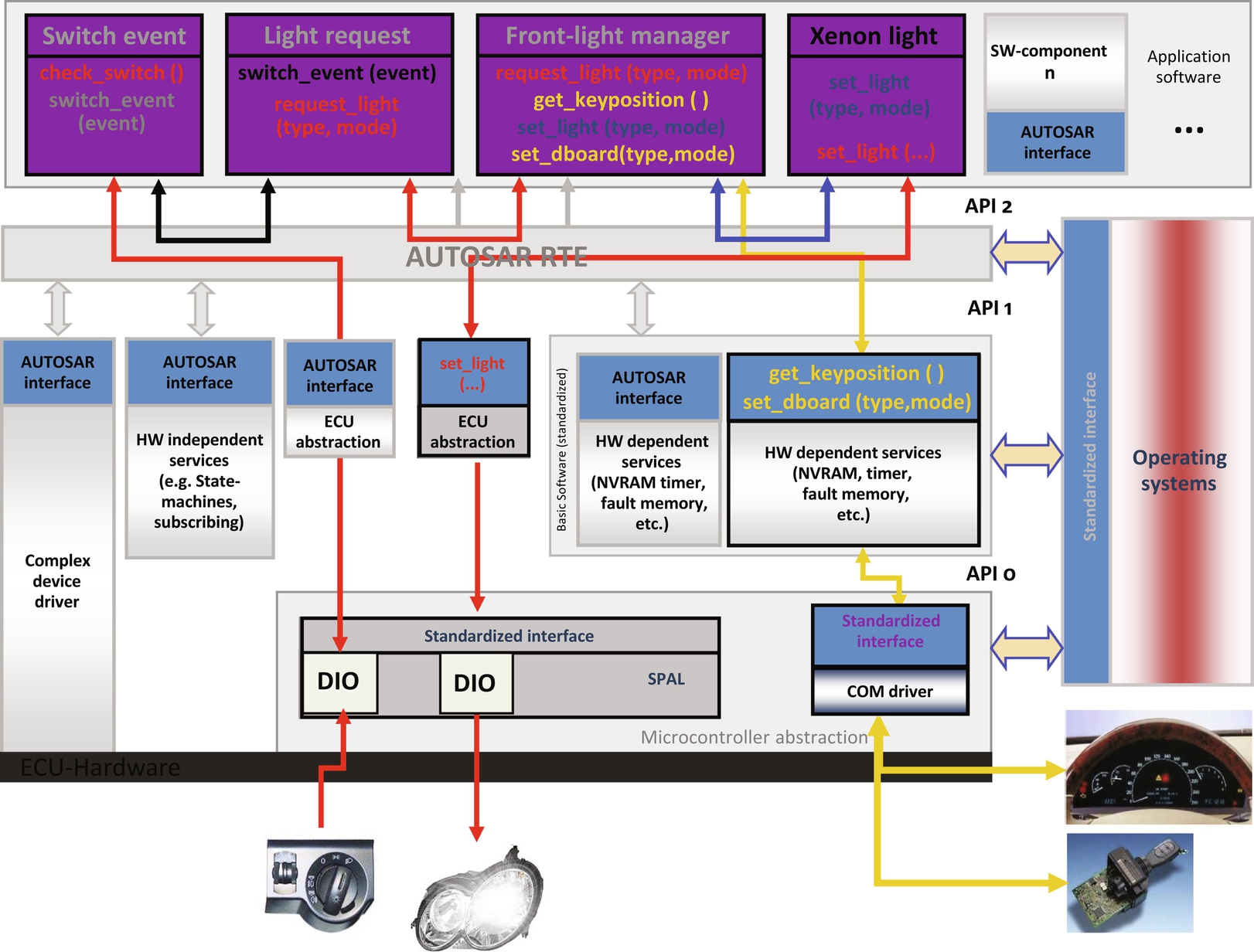
Embedded system development is about programming at the hardware level. But hardware abstraction layers (HALs) are a way to provide an interface between hardware and software so applications can be device independent. This is becoming more common in embedded systems. Basically, embedded applications access hardware through the HAL. The HAL encapsulates the peripherals of a microcontroller, and several API implementations can be provided at different levels of abstraction. An example HAL for an automotive application is shown in Fig. 19.

There are a few problems that a HAL attempts to address:
- • Complexity of peripherals and processors, this is hard for a real-time operating system (RTOS) to support out of the box, most RTOSs cover 20%–30% of the peripherals out of the box.
- • Packaging of the chip-mixing function—how does the RTOS work as you move from a standard device to a custom device?
- • The RTOS is basically the lowest common denominator, a HAL can support the largest number of processors. However, some peripherals, like an analog-to-digital converter (ADC) require custom support (peripherals work in either DMA mode or direct mode, and we need to support both).
The benefits of a HAL include:
- • Allowing easy migration between embedded processors.
- • Leveraging existing processor knowledgebase.
- • Creating code compliant with a defined programming interface, such as a standard application programming interface (API), a CAN driver source code, or an extension to a standard API, such as a higher level protocol over SCI communication (like a UDP) or even your own API.
As an example of this more advanced software architecture and a precursor to more detailed material to follow later, consider the case of an automobile “front light management” system as shown in Fig. 20. In this system, what happens if software components are running on different processors? Keep in mind that this automobile system must be a deterministic network environment. The CAN bus inside the car is not necessarily all the same CPU.

As shown in Fig. 21, we want to minimize the changes to the software architecture if we need to make a small change, like replacing a headlight. We want to be able to change the peripheral (changing the headlight or offering optional components as shown in Fig. 22) but not have to change anything else.

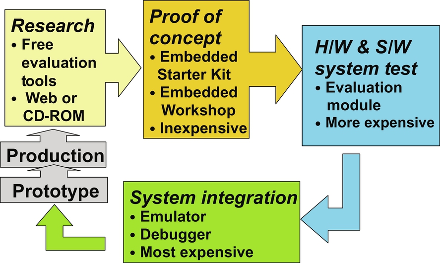
Finally, the embedded systems development flow follows a model similar to that shown in Fig. 23. Research is performed early in the process followed by a proof of concept and a hardware and software codesign and test. System integration follows this phase, where all of the hardware and software components are integrated together. This leads to a prototype system that is iterated until eventually a production system is deployed. We look into the details of this flow as we begin to dive deeper into the important phases of software engineering for embedded systems.