
Chapter 6: Data Management
In the previous chapter, you learned how to optimize your data layout to accelerate performance in query engines and manage the data optimally to reduce costs. This is a really important topic, but it is just one aspect of a data lake. As the volume of data increases, a data lake is used by different stakeholders – not only data engineers and software engineers but also data analysts, data scientists, and sales and marketing representatives. Sometimes, the original data is not easy to use for these stakeholders because the raw data may not be structured well. To make business decisions based on data quickly and effectively, it is important to manage, clean up, and enrich the data so that these stakeholders can understand the data correctly, find insights from the data without any confusion, correlate them, and drive their business based on data.
In this chapter, you will learn how to manage, clean up, and enrich the data in typical data requirements, and how to achieve this using AWS Glue. AWS Glue provides various functionalities that allow you to implement ETL logic easily. In addition, Apache Spark has lots of capabilities for different data operations. With AWS Glue, you can take advantage of both, which will help you make your data lake effective in real-world use cases.
In this chapter, we will cover the following topics:
- Normalizing data
- Deduplicating records
- Denormalizing tables
- Securing data content
- Managing data quality
Technical requirements
For this chapter, you will need the following resources:
- An AWS account
- An AWS IAM role
- An Amazon S3 bucket
All the sample code needs to be executed in a Glue runtime (for example, the Glue job system, Glue Interactive Sessions, a Glue Studio notebook, a Glue Docker container, and so on). If you do not have any preferences, we recommend using a Glue Studio notebook so that you can easily start writing code. To use a Glue Studio notebook, follow these steps:
- Open the AWS Glue console.
- Click AWS Glue Studio.
- Click Jobs.
- Under Create job, click Jupyter Notebook, then Create.
- For Job name, enter your preferred job name.
- For IAM Role, choose an IAM role where you have enough permission.
- Click Start notebook job.
- Wait for the notebook to be started.
- Write the necessary code and run the cells on the notebook.
Let’s begin!
Normalizing data
Data normalization is a technique for cleaning data. There are different techniques for normalizing data that make it easy to understand and analyze. This section covers the following techniques and use cases:
- Casting data types and map column names
- Inferring schemas
- Computing schemas on the fly
- Enforcing schemas
- Flattening nested schemas
- Normalizing scale
- Handling missing values and outliers
- Normalizing date and time values
- Handling error records
Let’s dive in!
Casting data types and map column names
In the context of data lakes, there can be a lot of different data sources. This may cause inconsistency in data types or column names. For example, when you want to join multiple tables where there is inconsistency, it can cause query errors or invalid calculations. To avoid such issues and make further analytics easier, it is a good approach to cast the data types and apply mapping to the data during the extract, transform, load (ETL) phase.
Let’s create a simple DataFrame as an example:
from pyspark.sql import Row
product = [
{'product_id': '00001', 'product_name': 'Heater', 'product_price': '250'}, {'product_id': '00002', 'product_name': 'Thermostat', 'product_price': '400'}]
df_products = spark.createDataFrame(Row(**x) for x in product)
df_products.printSchema()
df_products.show()
The preceding code returns the following output. You will notice that there are three columns and that all of them are of the string type:
root
|-- product_id: string (nullable = true)
|-- product_name: string (nullable = true)
|-- product_price: string (nullable = true)
+----------+------------+-------------+
|product_id|product_name|product_price|
+----------+------------+-------------+
| 00001| Heater| 250|
| 00002| Thermostat| 400|
+----------+------------+-------------+
In natural analysis, you may want to calculate the average price for all products. To support such analysis use cases, the columns, such as product_price, should be converted from string into integer.
Apache Spark supports type casting in Spark DataFrames. You can cast the type as an integer and rename the column’s name from product_price to price by running the following code:
from pyspark.sql.functions import col
df_mapped_dataframe = df_products
.withColumn("product_price", col("product_price").cast('integer')) .withColumnRenamed("product_price", "price")df_mapped_dataframe.printSchema()
df_mapped_dataframe.show()
The preceding code returns the following output. You will notice that the column’s name has been renamed to price and that the data type has been converted from string into integer, as expected:
root
|-- product_id: string (nullable = true)
|-- product_name: string (nullable = true)
|-- price: integer (nullable = true)
+----------+------------+-----+
|product_id|product_name|price|
+----------+------------+-----+
| 00001| Heater| 250|
| 00002| Thermostat| 400|
+----------+------------+-----+
You can achieve the same thing with SQL syntax as well. The following code registers the df_products DataFrame as a Hive table and runs a SELECT query against the table:
df_products.createOrReplaceTempView("products")df_mapped_sql = spark.sql("SELECT product_id, product_name, INT(product_price) as price from products")df_mapped_sql.printSchema()
df_mapped_sql.show()
The preceding code returns the following output. You will notice that you get the same result that you did with the DataFrame:
root
|-- product_id: string (nullable = true)
|-- product_name: string (nullable = true)
|-- price: integer (nullable = true)
+----------+------------+-----+
|product_id|product_name|price|
+----------+------------+-----+
| 00001| Heater| 250|
| 00002| Thermostat| 400|
+----------+------------+-----+
In the preceding tutorial, you used a Spark DataFrame to cast column types and rename columns.
On the other hand, an AWS Glue DynamicFrame provides the ApplyMapping transform so that you can cast and apply the mapping of column names and data types. The following example shows how to use the ApplyMapping transform:
from pyspark.context import SparkContext
from awsglue.context import GlueContext
from awsglue import DynamicFrame
glueContext = GlueContext(SparkContext.getOrCreate())
dyf = DynamicFrame.fromDF(df_products, glueContext, "from_df")
dyf = dyf.apply_mapping(
[
('product_id', 'string', 'product_id', 'string'), ('product_name', 'string', 'product_name', 'string'), ('product_price', 'string', 'price', 'integer')]
)
df_mapped_dyf = dyf.toDF()
df_mapped_dyf.printSchema()
df_mapped_dyf.show()
The preceding code returns the following output. As you can see, you get the same result that you did with the DataFrame:
root
|-- product_id: string (nullable = true)
|-- product_name: string (nullable = true)
|-- price: integer (nullable = true)
+----------+------------+-----+
|product_id|product_name|price|
+----------+------------+-----+
| 00001| Heater| 250|
| 00002| Thermostat| 400|
+----------+------------+-----+
As you have learned, you can use either a Spark DataFrame or Glue DynamicFrame for data type casting and column mapping.
Inferring schemas
Apache Spark can infer schemas from the content of data. With schema inference, you can create a DataFrame without passing the static schema structure.
When you read a CSV file without schema inference, you can set the inferSchema option to False. It is disabled by default. You can use the following code to create a DataFrame by reading from one sample CSV file located on Amazon S3:
df_infer_schema_false = spark.read.format("csv") .option("header", True) .option("inferSchema", False) .load("s3://covid19-lake/static-datasets/csv/CountyPopulation/County_Population.csv")df_infer_schema_false.printSchema()
The preceding code returns the following output. You will notice that all of the columns are recognized as being of the string type:
root
|-- Id: string (nullable = true)
|-- Id2: string (nullable = true)
|-- County: string (nullable = true)
|-- State: string (nullable = true)
|-- Population Estimate 2018: string (nullable = true)
When you set the inferSchema option to True, you must run following code:
df_infer_schema_true = spark.read.format("csv") .option("header", True) .option("inferSchema", True) .load("s3://covid19-lake/static-datasets/csv/CountyPopulation/County_Population.csv")df_infer_schema_true.printSchema()
The preceding code returns the following output. You will notice that the Id2 and Population Estimate 2018 columns are registered as the integer type instead of the string type:
root
|-- Id: string (nullable = true)
|-- Id2: integer (nullable = true)
|-- County: string (nullable = true)
|-- State: string (nullable = true)
|-- Population Estimate 2018: integer (nullable = true)
In this section, you learned that the inferSchema option manages the schema inference behavior to read CSV files.
It is a good idea to infer schemas from data when you do not want to define static schemas in advance and you want to define a schema from unpredictable data.
Computing schemas on the fly
A Spark DataFrame is a data representation in Apache Spark. It is powerful and widely used in a huge number of Spark clusters in various kinds of real-world use cases. A DataFrame is conceptually equivalent to a table, and it is optimized for relational database-like table operations such as aggregations and joins.
However, when you use a Spark DataFrame for ETL operations, you may face some typical issues. First, a DataFrame requires a schema to be provided before data is loaded. This can be a problem when you do not know or cannot predict the schema of the data in advance. Second, a DataFrame can have one schema per frame. This can be a problem when the same field in a frame has different types of values in multiple records. Even when you want to determine the type afterward, it is not possible. These issues often occur in messy data.
AWS Glue has a unique data representation called a DynamicFrame, which is similar to a Spark DataFrame. You can use it to convert a Spark DataFrame into a DynamicFrame and vice versa, but there are important differences between the two operations. First, in a Glue DynamicFrame, each record is self-describing. The Glue DynamicFrame computes a schema on-the-fly, so no schema is required initially. Second, a Glue DynamicFrame can have one schema per record, not per frame. The logical record in the DynamicFrame is called a DynamicRecord. When the same field in a DynamicFrame is of a different type in multiple DynamicRecords, the DynamicFrame allows you to determine the preferred types after loading the data.
Before trying DynamicFrame’s on-the-fly schema feature, you need to upload a sample file to your S3 bucket and create a table on the Glue Data Catalog. Follow these steps:
- Create a sample JSON Lines (JSONL) file:
{"id":"aaa","key":12}
{"id":"bbb","key":34}
{"id":"ccc","key":56}
{"id":"ddd","key":78}
{"id":"eee","key":"90"}
- Upload the sample file to your S3 bucket (replace the path with your S3 path):
$ aws s3 cp sample.json s3://path_to_sample_data/
- Create a Glue database:
$ aws glue create-database --database-input Name=choice
- Create a Glue crawler on s3://path_to_sample_data/:
$ aws glue create-crawler --name choice --database choice --role GlueServiceRole --targets '{"S3Targets":[{"Path":"s3:// path_to_sample_data/"}]}'
- Run the crawler (replace the IAM role with yours):
$ aws glue start-crawler --name choice
- After running the crawler, you will see the sample table in the catalog.
Here’s the schema of the sample table that was returned by the get-table AWS CLI command:
$ aws glue get-table --database-name choice --name sample --query Table.StorageDescriptor.Columns --output table
--------------------
| GetTable |
+-------+----------+
| Name | Type |
+-------+----------+
| id | string |
| key | string |
+-------+----------+
Now, we’re all set to create a DynamicFrame. You can create a DynamicFrame from the table definition on the Glue Data Catalog by running the following code:
from pyspark.context import SparkContext
from awsglue.context import GlueContext
glueContext = GlueContext(SparkContext.getOrCreate())
dyf_sample = glueContext.create_dynamic_frame.from_catalog(
database = "choice",
table_name = "sample")
dyf_sample.printSchema()
The preceding code returns the following output. You will notice that the key column is registered as a choice type. This means that key could be either of the int or string type. This happened because the Spark DataFrame schema recognizes key as an int type, but the Glue Data Catalog recognizes key as a string type:
root
|-- id: string
|-- key: choice
| |-- int
| |-- string
There are five records in the sample JSONL file. The values in the key field in the first four records are all integers, while at the end of the file, there is one record with a string value in that column.
AWS Glue DynamicFrames allow you to determine the schema after loading the data by introducing the concept of a choice type. To query the key column or to save the frame, you need to resolve the choice type first using the resolveChoice transform method. For example, you can run the resolveChoice transform with the cast:int option to convert those string values into int values:
dyf_sample_resolved = dyf_sample.resolveChoice(specs = [('key','cast:int')])dyf_sample_resolved.printSchema()
The output of printSchema is as follows:
root
|-- id: string
|-- key: int
You will notice that the key column is now recognized as int instead of choice or string.
As you have learned, DynamicFrames have unique on-the-fly schema capabilities and the choice type allows you to determine the schema after data load. This would be useful for ETL workloads where your data can include different data types.
Enforcing schemas
In an Apache Spark DataFrame, you need to set a static schema per frame. Similarly, in DynamicFrames you can enforce a static schema using the with_frame_schema method.
Let’s create a new DynamicFrame using the example data located on Amazon S3:
from pyspark.context import SparkContext
from awsglue.context import GlueContext
glueContext = GlueContext(SparkContext.getOrCreate())
dyf_without_schema = glueContext.create_dynamic_frame_from_options(
connection_type = "s3",
connection_options = {"paths": ["s3://awsglue-datasets/examples/us-legislators/all/events.json"]
},
format = "json"
)
dyf_without_schema.printSchema()
The schema is automatically recognized, as shown in the following code. You will notice that the start_date, end_date, and identifier columns are recognized as strings:
Root
|-- classification: string
|-- name: string
|-- end_date: string
|-- identifiers: array
| |-- element: struct
| | |-- scheme: string
| | |-- identifier: string
|-- id: string
|-- start_date: string
|-- organization_id: string
Now, let’s pass a static schema to the with_frame_schema method using the same data. Be careful not to pass the schema after schema computation. Do not execute the printSchema method before the with_frame_schema method since the printSchema method triggers schema computation and with_frame_schema is only available before schema computation:
from awsglue.gluetypes import Field, ArrayType, StructType, StringType, IntegerType
dyf_without_schema_tmp = glueContext.create_dynamic_frame_from_options(
connection_type = "s3",
connection_options = {"paths": ["s3://awsglue-datasets/examples/us-legislators/all/events.json"]
},
format = "json"
)
schema = StructType([
Field("id", StringType()), Field("name", StringType()), Field("classification", StringType()), Field("identifiers", ArrayType(StructType([ Field("schema", StringType()), Field("identifier", IntegerType())])),
),
Field("start_date", IntegerType()), Field("end_date", IntegerType()), Field("organization_id", StringType()),])
dyf_with_schema = dyf_without_schema_tmp.with_frame_schema(schema)
dyf_with_schema.printSchema()
The output of printSchema is now as follows:
root
|-- id: string
|-- name: long
|-- classification: string
|-- identifiers: array
| |-- element: struct
| | |-- schema: string
| | |-- identifier: int
|-- start_date: int
|-- end_date: int
|-- organization_id: string
You will notice that the start_date, end_date, and identifier columns are now recognized as integers instead of strings. Schema enforcement for a DynamicFrame is useful when you want to use a DynamicFrame but you do not want to rely on on-the-fly schemas or schema inference.
Flattening nested schemas
When you process unstructured/semi-structured data, you may see a schema that includes a deep nested struct or an array generated from applications. Here’s an example of a nested schema:
{"count": 2,
"entries": [
{"id": 1,
"values": {"k1": "aaa",
"k2": "bbb"
}
},
{"id": 2,
"values": {"k1": "ccc",
"k2": "ddd"
}
}
]
}
Typically, for most query engines, a nested schema introduces additional complexity for analytics. Also, for humans, it is not easy to read. To overcome that, you can flatten the schema. AWS Glue’s Relationalize transform helps you convert a deep nested schema into a flat schema:
from pyspark.context import SparkContext
from awsglue.context import GlueContext
glueContext = GlueContext(SparkContext.getOrCreate())
dyf = glueContext.create_dynamic_frame_from_options(
connection_type = "s3",
connection_options = {"paths": ["s3://path_to_nested_json/"]},format = "json"
)
dyf.printSchema()
dyf.toDF().show()
The output of printSchema is now as follows:
root
|-- count: int
|-- entries: array
| |-- element: struct
| | |-- id: int
| | |-- values: struct
| | | |-- k1: string
| | | |-- k2: string
The output of show is now as follows:
+-----+--------------------+
|count| entries|
+-----+--------------------+
| 2|[{1, {aaa, bbb}},...|
+-----+--------------------+
Then, you can perform a Relationalize transform on this nested schema:
from awsglue.transforms import Relationalize
dfc_root_table_name = "root"
dfc = Relationalize.apply(
frame = dyf,
staging_path = "s3://your-tmp-s3-path/",
name = dfc_root_table_name
)
dfc.keys()
The output of keys is now as follows:
dict_keys(['root', 'root_entries'])
The Relationalize transform returns a DynamicFrameCollection object. Now, you have two DynamicFrames inside this collection. Let’s extract both:
dyf_flattened_root = dfc.select(dfc_root_table_name)
dyf_flattened_root.printSchema()
dyf_flattened_root.toDF().show()
The output is now as follows:
root
|-- count: int
|-- entries: long
+-----+-------+
|count|entries|
+-----+-------+
| 2| 1|
+-----+-------+
Then, extract the second DynamicFrame inside the collection:
dyf_flattened_entries = dfc.select('root_entries')dyf_flattened_entries.printSchema()
dyf_flattened_entries.toDF().show()
The output is now as follows:

Figure 6.1 – Relationalized DynamicFrame
If you want to rejoin these two DynamicFrames, run the following code:
df_flattened_root = dyf_flattened_root.toDF()
df_flattened_entries = dyf_flattened_entries.toDF()
df_joined = df_flattened_root.join(df_flattened_entries)
df_joined.printSchema()
df_joined.show()
The output will be as follows:
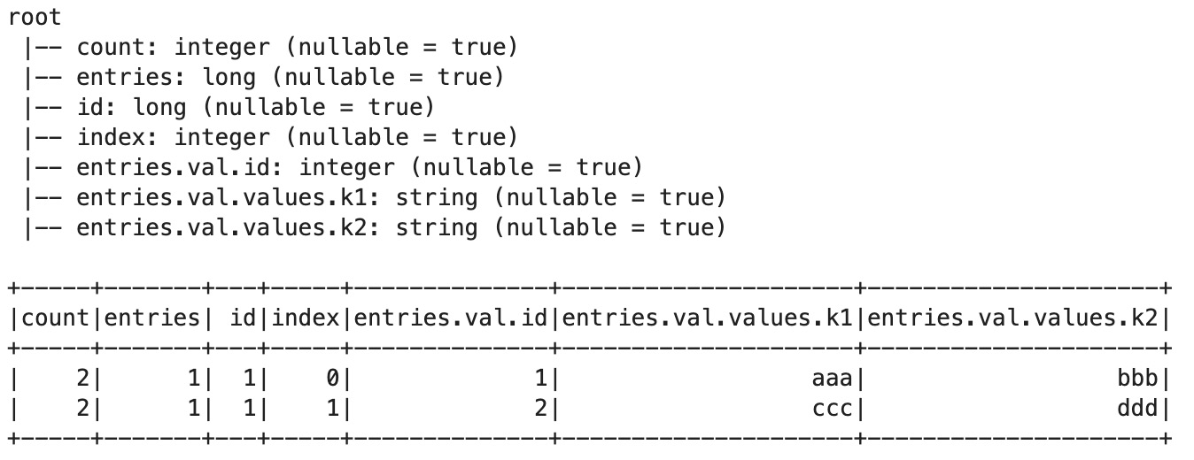
Figure 6.2 – Rejoined DynamicFrame
In this section, you learned that Relationalize returns a collection of DynamicFrames from deep nested data. It is useful for flattening nested data.
Normalizing scale
In the context of mathematics, machine learning (ML), or statistics, normalization is commonly used to prepare data on the same scale. Imagine that you have an Amazon review dataset and that each review has a star rating for an item. The value of the rating is 1 to 5 in the original data. On the other hand, most ML algorithms expect a value between 0 to 1. If you prefer to rescale data, you can use any typical normalization method, such as min-max normalization, mean normalization, and Z-score normalization.
AWS Glue DataBrew supports mechanisms such as mean normalization and Z-scale normalization. You can easily scale and normalize the values with a GUI.
Handling missing values and outliers
Real-world data typically includes missing values or outliers, and they sometimes cause invalid trends in analysis or unexpected results in ML.
With AWS Glue jobs, you can use the FillMissingValues transform to handle missing values in the dataset. The FillMissingValues transform has been built on top of an ML algorithm. It detects null values and empty strings as missing values in a specific column and adds a new column with values that are automatically predicted by the ML algorithm, such as linear regression and random forest.
With AWS Glue DataBrew, you can fill missing values with predefined sets such as average, median, custom value, empty string, last valid value, and others. You can also detect outliers and replace them with the rescaled values.
Normalizing date and time values
Real-world data uses different notations of date and time. In the US, It is common to use the MM/dd/yyyy format (for example, 12/25/2021), whereas in Europe, it is common to use the dd/MM/yyyy format (for example, 25/12/2021). Since they can be confused with each other, it is important to convert international use cases into a unified format.
Unix time (also known as epoch time or POSIX time) is used in various systems. It is the number of seconds that have elapsed since the Unix epoch, excluding leap seconds. The Unix time of 00:00, December 25, 2021, in UTC is 1640390400. Since it is hard for a human to read, typically, it is converted into a human-readable timestamp format in queries or dashboards.
ISO 8601 is an international standard that covers the worldwide exchange and communication of date- and time-related data. For example, the ISO 8601 format for the date and time of 00:00, December 25, 2021, in UTC is 2021-12-25T00:00:00+00:00.
In the case of international use cases, it is important to choose a timezone to show the data. Usually, an application needs to adjust the end user’s timezone. If you expect all the end users to be in a specific timezone, it may be also okay to store the timestamp within that specific timezone.
With AWS Glue, you can use any of Spark’s or Glue DynamicFrame’s methods to convert a specific date and time format into a timestamp type. Spark has various date and time functions, including unix_timestamp, date_format, to_unix_timestamp, from_unixtime, to_date, to_timestamp, from_utc_timestamp, and to_utc_timestamp.
The following is an example DataFrame that includes a timestamp record:
df_time_string = spark.sql("SELECT '2021-12-25 00:00:00' as timestamp_col") df_time_string.printSchema()
df_time_string.show()
The schema and the following data are returned by the preceding code:
root
|-- timestamp_col: string (nullable = false)
+-------------------+
| timestamp_col|
+-------------------+
|2021-12-25 00:00:00|
+-------------------+
Now, let’s convert the data type from a string type into a timestamp type using the DataFrame’s to_timestamp method:
from pyspark.sql.functions import to_timestamp, col
df_time_timestamp = df_time_string.withColumn(
"timestamp_col",
to_timestamp(col("timestamp_col"), 'yyyy-MM-dd HH:mm:ss'))
df_time_timestamp.printSchema()
df_time_timestamp.show()
The printSchema output is shown in the following code block. You will notice that the timestamp_col column is now recognized as timestamp instead of string:
root
|-- timestamp_col: timestamp (nullable = true)
+-------------------+
| timestamp_col|
+-------------------+
|2021-12-25 00:00:00|
+-------------------+
AWS Glue DynamicFrame also has the ApplyMapping transformation for casting values, including timestamps. The following code initiates Glue-related classes and converts the sample DataFrame into a DynamicFrame:
from pyspark.context import SparkContext
from awsglue.context import GlueContext
from awsglue import DynamicFrame
glueContext = GlueContext(SparkContext.getOrCreate())
dyf = DynamicFrame.fromDF(df_time_string, glueContext, "from_df")
The following code finds columns whose names contain timestamp_col dynamically and converts the string value in the column into the timestamp type:
mapping = []
for field in dyf.schema():
if field.name == 'timestamp_col':
mapping.append((
field.name, field.dataType.typeName(),
field.name, 'timestamp'
))
else:
mapping.append((
field.name, field.dataType.typeName(),
field.name, field.dataType.typeName()
))
dyf = dyf.apply_mapping(mapping)
df_time_timestamp_dyf = dyf.toDF()
df_time_timestamp_dyf.printSchema()
df_time_timestamp_dyf.show()
You will see the same result that you saw previously:
root
|-- timestamp_col: timestamp (nullable = true)
+-------------------+
| timestamp_col|
+-------------------+
|2021-12-25 00:00:00|
+-------------------+
Another typical date and time handling operation is to extract some values, such as the year, month, and day from the timestamp column dynamically. This is commonly done when you want to partition data into data lake storage based on the timestamp.
The following code extracts the year, month, and day values from the timestamp_col column:
from pyspark.sql.functions import year, month, dayofmonth
df_time_timestamp_ymd = df_time_timestamp
.withColumn('year', year("timestamp_col")) .withColumn('month', month("timestamp_col")) .withColumn('day', dayofmonth("timestamp_col"))df_time_timestamp_ymd.printSchema()
df_time_timestamp_ymd.show()
The preceding code returns the following output. You will notice that the DataFrame has three additional columns – year, month, and day – and that those columns contain the values that were extracted from the timestamp_col column:
root
|-- timestamp_col: timestamp (nullable = true)
|-- year: integer (nullable = true)
|-- month: integer (nullable = true)
|-- day: integer (nullable = true)
+-------------------+----+-----+---+
| timestamp_col|year|month|day|
+-------------------+----+-----+---+
|2021-12-25 00:00:00|2021| 12| 25|
+-------------------+----+-----+---+
With a Glue DataFrame, you can achieve the same by running the following code using the map function:
def add_timestamp_column(record):
dt = record["timestamp_col"]
record["year"] = dt.year
record["month"] = dt.month
record["day"] = dt.day
return record
dyf = dyf.map(add_timestamp_column)
df_time_timestamp_dyf_ymd = dyf.toDF()
df_time_timestamp_dyf_ymd.printSchema()
df_time_timestamp_dyf_ymd.show()
The preceding code returns the following output:
root
|-- timestamp_col: timestamp (nullable = true)
|-- year: integer (nullable = true)
|-- month: integer (nullable = true)
|-- day: integer (nullable = true)
+-------------------+----+-----+---+
| timestamp_col|year|month|day|
+-------------------+----+-----+---+
|2021-12-25 00:00:00|2021| 12| 25|
+-------------------+----+-----+---+
In this section, you learned that you can easily normalize the date/time format in both a Spark DataFrame and a Glue DynamicFrame. You can also extract year/month/value values from a timestamp. This is useful for time series data, as well as data layouts that use time-based partitioning.
Handling error records
If the data is corrupted, Apache Spark or AWS Glue may not be able to read the records successfully. This can cause missing values and invalid results.
If you want to manage such situations, the Glue DynamicFrame class can detect error records. The following code detects the error records and aborts the job when the error rate exceeds the threshold:
import sys
from pyspark.context import SparkContext
from awsglue.context import GlueContext
from awsglue.job import Job
from awsglue.utils import getResolvedOptions
ERROR_RATE_THRESHOLD = 0.2
glue_context = GlueContext(SparkContext.getOrCreate())
dyf = glue_context.create_dynamic_frame.from_options(
connection_type = "s3",
connection_options = {'paths': ['s3://your_input_data_path/']},format = "csv",
format_options={'withHeader': False})
dataCount = dyf.count()
errorCount = dyf.errorsCount()
errorRate = errorCount/(dataCount+errorCount)
print(f"error rate: {errorRate}")if errorRate > ERROR_RATE_THRESHOLD:
raise Exception(f"error rate {errorRate} exceeded threshold: {ERROR_RATE_THRESHOLD}")errorDyf = dyf.errorsAsDynamicFrame()
glue_context.write_dynamic_frame_from_options(
frame=errorDyf,
connection_type='s3',
connection_options={'path': 's3://your_error_frame_path/'},format='json'
)
In this section, you learned that Glue provides a set of capabilities that can help you handle typical error records. Based on your requirements, you can trigger an exception when the error rate exceeds the predefined threshold.
Deduplicating records
When you start analyzing the business data, you may find that it’s incorrect and that there are multiple different notations of the same record.
The following example table contains duplicates:
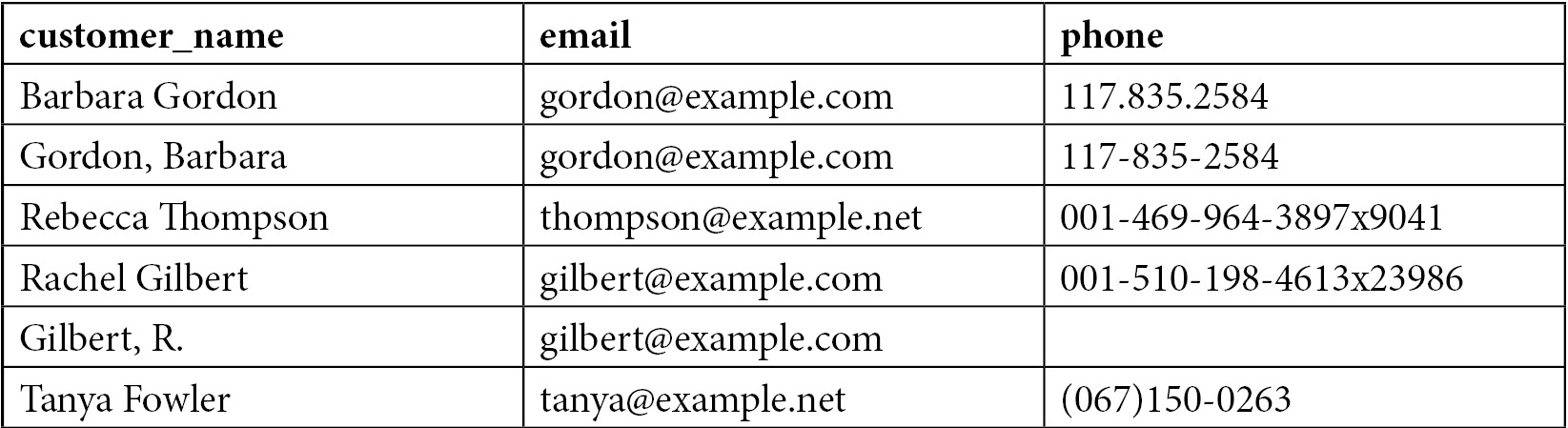
Figure 6.3 – Customer table with duplicates
As you may have noticed, there are only four unique records in the preceding table. Two records have two different notations, which causes duplication. If you analyze the data with these kinds of duplicated records, the result may include unexpected bias, so you will get an incorrect result.
With AWS Glue, you can use the FindMatches transform to find duplicated records. FindMatches is one of the ETL transforms provided in the Glue ETL library. With the FindMatches transform, you can match records and identify and remove duplicate records based on the ML model.
Let’s look at the end-to-end matching process:
- Register a table definition for your data in AWS Glue Data Catalog. You can use a Glue crawler, DDL, or the Glue catalog API to catalog your data.
- Create new Glue ML transforms using FindMatches. You need to choose the table created in step 1, give primary keys, and tune the balance between Recall and Precision and Lower cost and Accuracy.
- Train the FindMatches model by providing a labeling file that represents a perfect mapping of the records. You can estimate the quality of the model by reviewing the match quality metrics and uploading better labeling files if you want to improve the quality.
- Create and run an AWS Glue ETL job that uses your FindMatches transform.
You can find detailed steps in Integrate and deduplicate datasets using AWS Lake Formation (https://aws.amazon.com/blogs/big-data/integrate-and-deduplicate-datasets-using-aws-lake-formation-findmatches/).
Once you have completed the preceding steps, you will see the results shown in the following table:

Figure 6.4 – Deduplicated customer table
After matching the datasets, you will see that the result table represents the source table’s structure and data, as well as one more column: match_id. Each of the matched records displays the same match_id value. By utilizing these match_id values, you can filter with only distinct values to get unique records.
In this section, you learned that you can easily take advantage of the ML model in the FindMatches transform and deduplicate the same records efficiently.
Denormalizing tables
In this section, we will look at an example use case. There is a fictional e-commerce company that sells products and has a website that allows people to buy these products. There are three tables stored in the web system – two dimension tables, product and customer, and one fact table, sales. The product table stores the product’s name, category, and price. The customer table stores individual customer names, email addresses, and phone numbers. These email addresses and phone numbers are sensitive pieces of information that need to be handled carefully. When a customer buys a product, that activity is recorded in the sales table. One new record is inserted into the sales table every time a customer buys a product.
The following is the product dimension table:

Figure 6.5 – Product table
The following code can be used to populate the preceding sample data in a Spark DataFrame:
df_product = spark.createDataFrame([
(11, "Introduction to Cloud", "Ebooks", 15),
(12, "Best practices on data lakes", "Ebooks", 25),
(21, "Data Quest", "Video games", 30),
(22, "Final Shooting", "Video games", 20)
], ['product_id', 'product_name', 'category', 'price'])
df_product.show()
df_product.createOrReplaceTempView("product")The preceding code returns the following output:

Figure 6.6 – DataFrame for the Product table
The following is the customer dimension table:

Figure 6.7 – Customer table
The following code can be used to populate the preceding sample data in a Spark DataFrame:
df_customer = spark.createDataFrame([
("A103", "Barbara Gordon", "[email protected]", "117.835.2584"), ("A042", "Rebecca Thompson", "[email protected]", "001-469-964-3897x9041"), ("A805", "Rachel Gilbert", "[email protected]", "001-510-198-4613x23986"), ("A404", "Tanya Fowler", "[email protected]", "(067)150-0263")], ['uid', 'customer_name', 'email', 'phone'])
df_customer.show(truncate=False)
df_customer.createOrReplaceTempView("customer")The preceding code returns the following output:
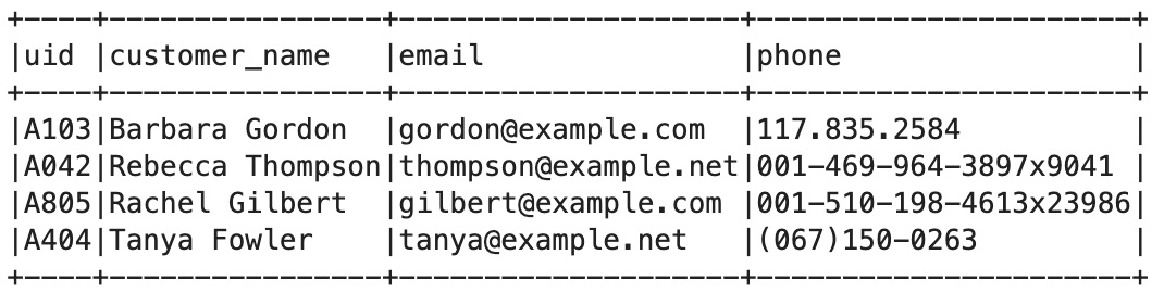
Figure 6.8 – DataFrame for the Customer table
The following is the sales fact table (the purchased_by field is the foreign key for the uid field in the customer table):
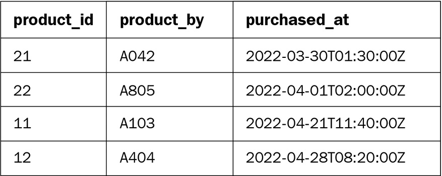
Figure 6.9 – Sales table
The following code can be used to populate the preceding sample data in a Spark DataFrame:
df_sales = spark.createDataFrame([
(21, "A042", "2022-03-30T01:30:00Z"),
(22, "A805", "2022-04-01T02:00:00Z"),
(11, "A103", "2022-04-21T11:40:00Z"),
(12, "A404", "2022-04-28T08:20:00Z")
], ['product_id', 'purchased_by', 'purchased_at'])
df_sales.show(truncate=False)
df_sales.createOrReplaceTempView("sales")The preceding code returns the following output:

Figure 6.10 – DataFrame for the Sales table
These tables are well-designed and normalized in the context of relational databases. However, this means that the data analyst always needs to join the tables for analysis.
For example, if you want to find the names of customers who bought products in April, you need to join the customer and sales tables, then filter with the purchased_at column:
Spark.sql("SELECT customer_name, purchased_at FROM sales JOIN customer ON sales.purchased_by=customer.uid WHERE purchased_at LIKE '2022-04%'").show()The preceding code returns the following output:

Figure 6.11 – Customers who bought products in April
It is not critical when the tables are small, but if the tables are large, you will spend an unnecessarily long time joining tables. In addition, joins can cause huge memory consumption in well-known analytic engines, including Apache Spark, and it sometimes causes out-of-memory (OOM) errors.
Denormalization is one of the typical optimization techniques that has fewer joins and simpler queries. Once you denormalize the table by joining the source tables in advance, you won’t need to join the tables in the analysis phase, and your query syntax will be simpler. The disadvantage of denormalization is that you will need to have some redundancy in the data, and you will have to think about how to keep the denormalized table up to date.
Let’s denormalize the four preceding tables into a destination table:
df_product_sales = df_product.join(
df_sales,
df_product.product_id == df_sales.product_id
)
df_destination = df_product_sales.join(
df_customer,
df_product_sales.purchased_by == df_customer.uid
)
df_destination.createOrReplaceTempView("destination")df_destination.select('product_name','category','price','customer_name','email','phone','purchased_at').show()The following table shows some of the columns in the destination table:

Figure 6.12 – DataFrame for the Destination table
Once you have created the destination table, you can easily find the name of people who purchased products in April without joining all the relevant tables every time:
spark.sql("SELECT product_name,category,price,customer_name,email,phone,purchased_at FROM destination WHERE purchased_at LIKE '2022-04%'").show()Here is the output of the preceding code:
The preceding code returns the following output:
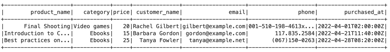
Figure 6.13 – The Destination table with customers who bought products in April 2022
In this section, you learned that tables can be denormalized by joining them. This is useful for optimizing performance in analytics workloads as it avoids having multiple joins in queries. However, if you denormalize the tables and store them on data lakes, they will be a little bit harder to maintain because you need to repeat the denormalization process whenever the source tables are changed. You will need to decide on a direction based on your workload.
Securing data content
In the context of a data lake, security is a “job zero” priority. In Chapter 8, Data Security, we will dive deep into security. In this section, we cover basic ETL operations that secure data. The following common techniques can be used to hide confidential values from data:
- Masking values
- Hashing values
In this section, you will learn how to mask/hash values that are included in your data.
Masking values
In business data lakes, the data can contain sensitive data, such as people’s names, phone numbers, credit card numbers, and so on. Data security is an important aspect of data lakes. There are different approaches to handling such data securely. It is a good idea to just drop the sensitive data when you collect the data from data sources when you won’t use the sensitive data in analytics. It is also common to manage access permissions on certain columns or records of the data. Another approach is to mask the data entirely or partially when you want to keep it confidential but also keep the same format – for example, the number of digits or characters.
With AWS Glue, you can mask a specific column using Spark DataFrame’s withColumn method by replacing the text based on a regular expression:
from pyspark.sql.functions import regexp_replace
df_masked = df_destination.withColumn("phone", regexp_replace("phone", r'(d)', '*'))df_masked.select('product_name','category','price','customer_name','email','phone','purchased_at').show()Once you have masked the data, you will see the following output. You will notice that only the numbers have been replaced in the phone column:

Figure 6.14 – The Destination table contains masked phone numbers
In terms of personally identifiable information (PII) data, AWS Glue has a native capability for detecting the PII data dynamically based on the data. At the time of writing, it can detect the following 16 entities:
- ITIN (US)
- Passport Number (US)
- US Phone
- Credit Card
- Bank Account (US, Canada)
- US Driving License
- IP Address
- MAC Address
- DEA Number (US)
- HCPCS Code (US)
- National Provider Identifier (US)
- National Drug Code (US)
- Health Insurance Claim Number (US)
- Medicare Beneficiary Identifier (US)
- CPT Code (US)
If you want to detect the PII data and mask it based on the detected result, you can use the following code:
entities_filter = [] # Empty list means we detect all entities.
sample_fraction = 1.0 # 100%
threshold_fraction = 0.8 # At least 80% of rows for a given column should contain the same entity in order for the column to be classified as that entity.
transformation_ctx = ""
stage_threshold = 0
total_threshold = 0
recognizer = EntityRecognizer()
results = recognizer.classify_columns(frame=dyf, entities_filter=entities_filter, sample_fraction=sample_fraction, threshold_fraction=threshold_fraction, stageThreshold=stage_threshold, totalThreshold=total_threshold)
for key in results:
for recognized_value in results[key]:
# Mask CREDIT_CARD, PHONE_NUMBER and IP_ADDRESS columns
if recognized_value in ["CREDIT_CARD", "PHONE_NUMBER", "IP_ADDRESS"]:
df = df.withColumn(key, regexp_replace(key, r'(d)', '*'))
In this section, you learned that, with AWS Glue, you can easily mask your data. Glue’s PII detection helps you dynamically choose the confidential columns and mask them.
Hashing values
Another way to keep data secure but still make some analytic queries available is hashing. Hashing is the process of passing data to a hash function and converting it into the result. Hashed data is always the same length, regardless of the amount of original data. MD5 is one of the common hash mechanisms for returning a 128-bit checksum as a hex string of the value. SHA2 returns a checksum from the SHA-2 family (for example, SHA-224, SHA-256, SHA-384, or SHA-512) as a hex string of the value.
These hashing algorithms are one-way, which means they can’t be reversed. One possible way to retrieve the original value from a hashed result is to brute-force it. A brute-force attack is commonly performed by generating all the possible values, making a hash of them, and then comparing the generated hashes with the original hash result.
Let’s compute a hash for one column in the table. Apache Spark supports hashing algorithms such as MD5, SHA, SHA1, SHA2, CRC32, and xxHash. Here, we will use SHA2 to hash the email column:
from pyspark.sql.functions import sha2
df_hashed = df_masked.withColumn("email", sha2("email", 256))df_hashed.select('product_name','category','price','customer_name','email','phone','purchased_at').show()Once you have hashed the data, you will see the following output. You will notice that only the email addresses have been hashed in the email column:

Figure 6.15 – The Destination table with hashed email addresses
If you want to integrate PII detection with hashing, you can use the following code:
entities_filter = [] # Empty list means we detect all entities.
sample_fraction = 1.0 # 100%
threshold_fraction = 0.8 # At least 80% of rows for a given column should contain the same entity in order for the column to be classified as that entity.
transformation_ctx = ""
stage_threshold = 0
total_threshold = 0
recognizer = EntityRecognizer()
results = recognizer.classify_columns(frame=dyf, entities_filter=entities_filter, sample_fraction=sample_fraction, threshold_fraction=threshold_fraction, stageThreshold=stage_threshold, totalThreshold=total_threshold)
for key in results:
for recognized_value in results[key]:
# Hash DRIVING_LICENSE, PASSPORT_NUMBER, and USA_ITIN columns using SHA-2
if recognized_value in ["DRIVING_LICENSE", "PASSPORT_NUMBER", "USA_ITIN"]:
df = df.withColumn(key, sha2(key, 256))
In this section, you learned that, similar to masking, you can easily hash your data with AWS Glue.
Managing data quality
When you build a modern data architecture from different data sources, the incoming data may contain incorrect, missing, or malformed data. This can make data applications fail. It can also result in incorrect business decisions due to incorrect data aggregations. However, it can be hard for you to evaluate the quality of the data if there is no automated mechanism. Today, it is important to manage data quality by applying predefined rules and verifying if the data meets those criteria or not.
Different frameworks can be used to monitor data quality. In this section, we will introduce two mechanisms: AWS Glue DataBrew data quality rules and DeeQu.
AWS Glue DataBrew data quality rules
Glue DataBrew data quality rules allow you to manage data quality to detect typical data issues easily. In this section, we will use a human resources dataset (https://eforexcel.com/wp/downloads-16-sample-csv-files-data-sets-for-testing/).
Follow these steps to manage data quality with Glue DataBrew:
- Create a data quality ruleset against your dataset.
- Create data quality rules. You can define multiple data quality rules here – for example, a rule to make sure that row count is correct and expected, there are no duplicate records, and so on.
- Create and run a profile job with the ruleset.
- Inspect the data quality rule’s validation results.
If data quality issues are detected by the rules, you can run DataBrew jobs to clean up the data and rerun the data quality checks.
You can find detailed steps in Enforce customized data quality rules in AWS Glue DataBrew (https://aws.amazon.com/blogs/big-data/enforce-customized-data-quality-rules-in-aws-glue-databrew/).
DeeQu
DeeQu, an open source data quality library, addresses data quality monitoring requirements and can scale to large datasets. DeeQu is built on top of Apache Spark to define “unit test for data.” With DeeQu, you can populate data quality metrics and define data quality rules easily.
DeeQu version 2.x runs with Spark 3.1, as well as with AWS Glue 3.0 jobs. Follow these steps before running any DeeQu code:
- Download the DeeQu 2.x JAR file from the Maven repository (https://mvnrepository.com/artifact/com.amazon.deequ/deequ/2.0.0-spark-3.1).
- Download the PyDeeQu 1.0.1 Wheel file from pypi.org (https://pypi.org/project/pydeequ/).
- Upload the JAR file and the Wheel file to your S3 bucket.
- Configure library dependencies. When you use the Glue job system, configure the --extra_jars and --extra_py_files parameters with the S3 paths of the JAR/Wheel files. When you use Glue Studio Notebook or Glue Interactive Sessions, configure %extra_jars and %extra_py_files, like so:
%extra_jars s3://path_to_your_lib/deequ-2.0.0-spark-3.1.jar
%extra_py_files s3://path_to_your_lib/pydeequ-1.0.1-py3-none-any.whl
- First, let’s initialize SparkSession and generate some sample data:
import pydeequ
from pyspark.sql import SparkSession
spark = (SparkSession
.builder
.config("spark.jars.packages", pydeequ.deequ_maven_coord)
.config("spark.jars.excludes", pydeequ.f2j_maven_coord)
.getOrCreate())
df = spark.createDataFrame([
(1, "Product A", "awesome thing.", "high", 2),
(2, "Product B", "available at http://producta.example.com", None, 0),
(3, None, None, "medium", 6),
(4, "Product D", "checkout https://productd.example.org", "low", 10),
(5, "Product E", None, "high", 18)
], ['id', 'productName', 'description', 'priority', 'numViews'])
- Now, let’s run the analyzer to measure the metrics in the sample data:
from pydeequ.analyzers import *
analysisResult = AnalysisRunner(spark)
.onData(df)
.addAnalyzer(Size())
.addAnalyzer(Completeness("id"))
.addAnalyzer(Completeness("productName"))
.addAnalyzer(Maximum("numViews"))
.addAnalyzer(Mean("numViews"))
.addAnalyzer(Minimum("numViews"))
.run()
analysisResult_df = AnalyzerContext.successMetricsAsDataFrame(spark, analysisResult)
analysisResult_df.show()
The preceding code returns the following output:
+-------+-----------+------------+-----+
| entity| instance| name|value|
+-------+-----------+------------+-----+
|Dataset| *| Size| 5.0|
| Column| id|Completeness| 1.0|
| Column|productName|Completeness| 0.8|
| Column| numViews| Maximum| 18.0|
| Column| numViews| Mean| 7.2|
| Column| numViews| Minimum| 0.0|
+-------+-----------+------------+-----+
- Now, let’s apply a verification check to understand if the data meets the predefined quality rules:
from pydeequ.checks import *
from pydeequ.verification import *
check = Check(spark, CheckLevel.Warning, "Review Check")
checkResult = VerificationSuite(spark)
.onData(df)
.addCheck(
# we expect 5 row
check.hasSize(lambda x: x == 5)
# should never be NULL
.isComplete("id")
# should not contain duplicates
.isUnique("id")
# should never be NULL
.isComplete("productName")
# should only contain the values "high", "medium", and "low"
.isContainedIn("priority", ["high", "medium", "low"])
# should not contain negative values
.isNonNegative("numViews")
# at least half of the descriptions should contain a url
.containsURL("description", lambda x: x >= 0.5)
# half of the items should have less than 10 views
.hasApproxQuantile("numViews", ".5", lambda x: x <= 10))
.run()
checkResult_df = VerificationResult.checkResultsAsDataFrame(spark, checkResult)
checkResult_df.show()
The preceding code returns the following output:
+------------+-----------+------------+--------------------+-----------------+--------------------+
| check|check_level|check_status| constraint|constraint_status| constraint_message|
+------------+-----------+------------+--------------------+-----------------+--------------------+
|Review Check| Warning| Warning|SizeConstraint(Si...| Success| |
|Review Check| Warning| Warning|CompletenessConst...| Success| |
|Review Check| Warning| Warning|UniquenessConstra...| Success| |
|Review Check| Warning| Warning|CompletenessConst...| Failure|Value: 0.8 does n...|
|Review Check| Warning| Warning|ComplianceConstra...| Success| |
|Review Check| Warning| Warning|ComplianceConstra...| Success| |
|Review Check| Warning| Warning|containsURL(descr...| Failure|Value: 0.4 does n...|
|Review Check| Warning| Warning|ApproxQuantileCon...| Success| |
+------------+-----------+------------+--------------------+-----------------+--------------------+
When you want to see all the messages provided by the verification, you can run the following code:
checkResult_df.show(truncate=False)
The preceding code returns the following output:

Figure 6.16 – DeeQU data quality check result
In this section, you learned that Glue DataBrew and DeeQu help you analyze and validate data quality in your dataset.
Summary
In this chapter, you learned how to manage, clean up, and enrich your data using various functionalities available on AWS Glue and Apache Spark. In terms of normalizing data, you looked at several techniques, including schema enforcement, timestamp handling, and others. To deduplicate records, you experimented with using ML transforms with a sample dataset, while to denormalize tables, you joined multiple tables and enriched the data to optimize the analytic workload. When learning about masking and hashing values, you performed basic ETL to improve security. Moreover, you learned that Glue PII Detection helps you choose confidential columns dynamically. Finally, you learned how to manage data quality with Glue DataBrew data quality rules and DeeQu.
In the next chapter, you will learn about the best practices for managing metadata on data lakes.