
Chapter 4: Data Preparation
In the previous chapter, we explored fundamental concepts surrounding data ingestion and how we can leverage AWS Glue to ingest data from various sources, such as file/object stores, JDBC data stores, streaming data sources, and SaaS data stores. We also discussed different features of AWS Glue ETL, such as schema flexibility, schema conflict resolution, advanced ETL transformations and extensions, incremental data ingestion using job bookmarks, grouping, and workload partitioning using bounded execution in detail with practical examples. Doing so allowed us to understand how each of these features can be used to ingest data from data stores in specific use cases.
In this chapter, we will be introducing the fundamental concepts related to data preparation, different strategies that can help choose the right service/tool for a specific use case, visual data preparation, and programmatic data preparation using AWS Glue.
Upon completing this chapter, you will be able to explain how to perform data preparation operations in AWS Glue using a visual interface and source code. You will also be able to articulate different features of AWS Glue DataBrew, AWS Glue Studio, and AWS Glue ETL. You will also be able to write simple ETL scripts in AWS Glue ETL to prepare the data using some of the most popular transformations and extensions. Finally, you will be able to articulate the importance of planning and the different factors that must be taken into consideration while choosing a tool/service to implement a data preparation workflow.
In this chapter, we will cover the following topics:
- Introduction to data preparation
- Data preparation using AWS Glue
- Selecting the right service/tool
Now, let’s dive into the fundamental concepts of data preparation and understand how data preparation can be done using AWS Glue and the different services/tools we can utilize to perform data preparation tasks quite easily.
Technical requirements
Please refer to the Technical requirements section in Chapter 3, Data Ingestion, as they are the same for this chapter as well.
In the upcoming sections, we will be discussing the fundamental concepts of data preparation, the importance of data preparation, and how we can prepare data using different tools/services in AWS Glue.
Introduction to data preparation
Data preparation can be defined as the process of sanitizing and normalizing the dataset using a combination of transformations to prepare the data for downstream consumers. In a typical data integration workflow, prepared data is consumed by analytics applications, visualization tools, and machine learning pipelines. It is not uncommon for the prepared data to be ingested by other data processing pipelines, depending on the requirements of the consuming entity.
When we consider a typical data integration workflow, quite often, data preparation is one of the more challenging and time-consuming tasks. It is important to ensure the data is prepared correctly according to the requirements as this impacts the subsequent steps in the data integration workflow significantly.
The complexity of the data preparation process depends on several factors, such as the schema of the source data, schema drift, the volume of data, the transformations to be applied to obtain the data in the required schema, and the data format, to name a few. It is important to account for these factors while planning and designing the data preparation steps of the workflow to ensure the quality of the output data and to avoid a garbage in, garbage out (GIGO) situation.
Now that we know the fundamental concepts and the importance of the data preparation steps in a data integration workflow, let’s explore how we can leverage AWS Glue to perform data preparation tasks.
Data preparation using AWS Glue
It is normal for data to grow continuously over time in terms of volume and complexity, considering the huge number of applications and devices generating data in a typical organization. With this ever-growing data, a tremendous amount of resources are required to ingest and prepare this data – both in terms of manpower and compute resources.
AWS Glue makes it easy for individuals with varying levels of skill to collaborate on data preparation tasks. For instance, novice users with no programming skills can take advantage of AWS Glue DataBrew (https://aws.amazon.com/glue/features/databrew/), a visual data preparation tool that allows data engineers/analysts/scientists to interact with and prepare the data using a variety of pre-built transformations and filtering mechanisms without writing any code.
While AWS Glue DataBrew is a great tool for preparing data using a graphical user interface (GUI), there are some use cases where the built-in transformations may not be flexible enough or the user may prefer a programmatic approach to prepare data over using the GUI-based approach. In such cases, AWS Glue enables users to prepare data using AWS Glue ETL. Users can leverage AWS Glue Studio – AWS Glue’s new graphical interface – to author, execute, and monitor ETL workloads. Although Glue Studio offers a GUI, users may still require programmatic knowledge of AWS Glue’s transformation extensions and APIs to implement data preparation workloads, especially when implementing custom transformations using SQL or source code.
Now that we know about the different data preparation options that are available in AWS Glue, let’s dive deep into each of them while looking at practical examples to understand them.
Visual data preparation using AWS Glue DataBrew
AWS Glue makes it possible to prepare data using a visual interface through AWS Glue DataBrew. As mentioned previously, AWS Glue DataBrew is a visual data preparation tool wherein users can leverage over 250 pre-built transformations to filter, shape, and refine data according to their requirements. AWS Glue DataBrew makes it easy to gather insights from raw data, regardless of the level of technical skill that the individuals interacting with the data have. More importantly, since DataBrew is serverless, users can explore and reshape terabytes of data without creating expensive long-running clusters, thus eliminating any administrative overhead involved in managing infrastructure.
Getting started with AWS Glue DataBrew is quite simple. To use DataBrew, you can create a project and connect it to a data store to obtain raw data. AWS Glue DataBrew can ingest raw data from Amazon S3, Amazon Redshift, JDBC data stores (including on-premise database servers), and AWS Data Exchange. We can also ingest data from external data stores such as Snowflake. You can even upload a file directly from the AWS Glue DataBrew console and specify an Amazon S3 location to store this uploaded file. At the time of writing, AWS Glue DataBrew supports the CSV, TSV, JSON, JSONL, ORC, Parquet, and XLSX file formats.
AWS Glue DataBrew can also ingest data from a wide range of external Software-as-a-Service (SaaS) providers via Amazon AppFlow. There are several external SaaS providers supported via Amazon AppFlow, including Amplitude, Datadog, Google Analytics, Dynatrace, Marketo, Salesforce, ServiceNow, Slack, and Zendesk, to name a few. This feature enables users to prepare the data by applying the necessary transformations while interacting with the data on a visual interface. This data can be further integrated with datasets from other data stores or SaaS applications. This helps the users take a holistic approach to analyzing and gathering insights from their datasets, which have been spread across different data stores or SaaS platforms. The following screenshot outlines the grid-like visual interface and different options available in the AWS Glue DataBrew project workspace:

Figure 4.1 – AWS Glue DataBrew project workspace
Once a project has been created and a dataset has been attached to the project, you can specify the AWS IAM role that can be used by this project to interact with other AWS services and a sampling strategy. This includes specifying the number of rows the visual editor has to load and whether these rows can be chosen at random or whether they have to be from the beginning or the end of the dataset.
After creating the project, AWS Glue DataBrew loads the project workspace and you will see your data in a grid-like interface (Figure 4.1). You can explore the data with ease using the project workspace and you will also be able to gain insights into each column using the statistics populated under the column name in the interface. Detailed statistics can be viewed for individual columns by clicking on the column name. By doing this, AWS Glue DataBrew generates insights based on the sample data that’s been loaded into the project workspace and displays them in the Column details panel on the right-hand side of the workspace.
The following screenshot shows the list of recommendations that were generated for the human_rights column in the sample dataset after it was loaded into the AWS Glue DataBrew project workspace:
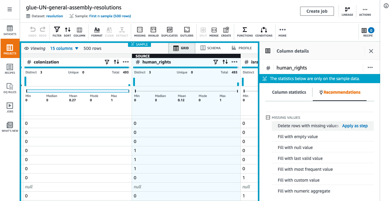
Figure 4.2 – AWS Glue DataBrew – recommended transformations
Based on the data type and the sample data that’s loaded into the workspace, AWS Glue DataBrew also generates a list of recommended transformations that can be applied. For instance, if the values for a specific column in the dataset are missing, the list of recommended transformations includes different strategies to handle missing values, such as deleting rows with missing values, filling with an empty value, filling with the last valid value, filling with the most frequent value, and filling with a custom value. To apply one of these transforms, all we have to do is click Apply as step next to the transform.
As we make changes by applying different transformations, AWS Glue DataBrew captures the sequence of transformations that have been applied and builds a recipe. You can click on the column name and select a transformation from the top ribbon to apply a transformation for that column. Once you are happy with the recipe that’s been generated, you can publish this recipe and it will be saved in AWS DataBrew (Figure 4.2a). This recipe can be downloaded as a JSON file and can be reused by importing the file as a new recipe in DataBrew. This is useful when you want to share the recipe with DataBrew users in other AWS accounts:
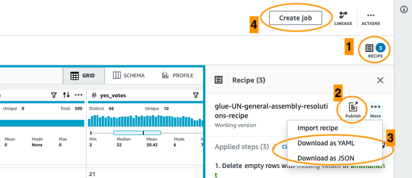
Figure 4.3 – Options to create, publish, and import/export recipes
In the preceding screenshot, several options are highlighted. Option 1 allows us to toggle the sidebar, which displays the current version of the recipe. The same recipe can be published using option 2. A recipe can be exported or imported using option 3. Finally, option 4 allows us to create a job from the recipe. Now that we know how to build, export, and import a recipe, let’s explore different types of jobs in AWS Glue DataBrew.
Recipe jobs
A recipe can be used to create a recipe job in AWS Glue DataBrew, which will allow you to run the steps on your dataset (refer to option 4 in Figure 4.3). The job can be set up to run on-demand or at regular intervals by specifying a schedule. At the time of writing, AWS Glue DataBrew allows you to write transformed data to Amazon S3, Amazon Redshift, and JDBC data. Additional settings can be specified for the job, depending on the type of output destination data store.
For instance, if you are writing the data to an Amazon S3 location, you can specify options such as output format, compression codec, and output encryption using AWS KMS. The list of available options changes with the type of output data store selected. Other configuration items can be set for the job run, such as Maximum number of units (maximum number of DataBrew nodes that can be used), Number of retries, Job timeout (in minutes), and CloudWatch logs for the job run.
Profile jobs
In the previous section, you learned how to define a recipe and create a job from this recipe. Wouldn’t it be great if most of the heavy lifting involved in understanding the data is handled by AWS Glue DataBrew so that we can plan the transformations better? AWS Glue DataBrew has another type of job called a profile job that addresses this exact issue. A profile job can be defined to evaluate the dataset and generate statistics and a summary that will help us understand the data better. This will, in turn, help us decide the type of transformations required to prepare the data.
A profile job run generates a data profile in AWS Glue DataBrew that contains a summary of the dataset and statistics for each column and any advanced summaries selected by the user. Profile jobs allow users to generate a correlations summary of different numeric columns available. It also allows you to profile the dataset based on advanced rules such as personally identifiable information (PII) detection. The dataset is evaluated using pre-built rules that analyze the column names and the values to flag any potential PII data in a given dataset. This is extremely helpful to make sure the dataset complies with data governance policies set forth by the organization or an external governing body.
The following screenshot shows what a sample data profile looks like:

Figure 4.4 – Data profile overview
In the lower half of the preceding screenshot, we can see that AWS Glue DataBrew has generated different summaries of the dataset based on the data types of the columns in the dataset. For instance, we can see a value distribution chart and the minimum, maximum, mean, median, mode, standard deviation, and other statistics for numeric columns. The summary also captures any missing data. We can use these pieces of information and design appropriate transformations in the recipe job to filter and reshape data based on our requirements.
Now that we know how profile jobs can be used to generate statistics and summaries for a given dataset, let’s learn how to enrich these summaries with information based on user-defined rules.
Controlling data quality using DQ Rules
AWS Glue DataBrew allows us to define a ruleset that governs the quality of the dataset based on specified rules. The dataset is evaluated against the user-defined rules and violations are flagged in the data profile generated by the profile job run. This allows us to enrich the data profile with additional information based on the custom rules defined.
Upon creating a dataset in AWS Glue DataBrew, you can navigate to the DQ Rules option in the navigation panel and define a new ruleset for the dataset that’s been created.
A data quality (DQ) ruleset is a collection of rules that defines the data quality for the dataset. This is achieved by comparing different data metrics with expected values. Once a ruleset has been defined, we can associate this ruleset with a profile job. After the job run, we will be able to see additional information under the Data quality rules tab in the generated data profile. This view includes the list of user-defined rules that were evaluated and a summary of whether all the columns adhered to these rules.
The following screenshot shows that the sample dataset was evaluated against two user-defined rules. The dataset passed the checks for one rule (Check Dataset For Duplicate Rows) and a few columns failed the checks for the other rule (Check All Columns For Missing Values):
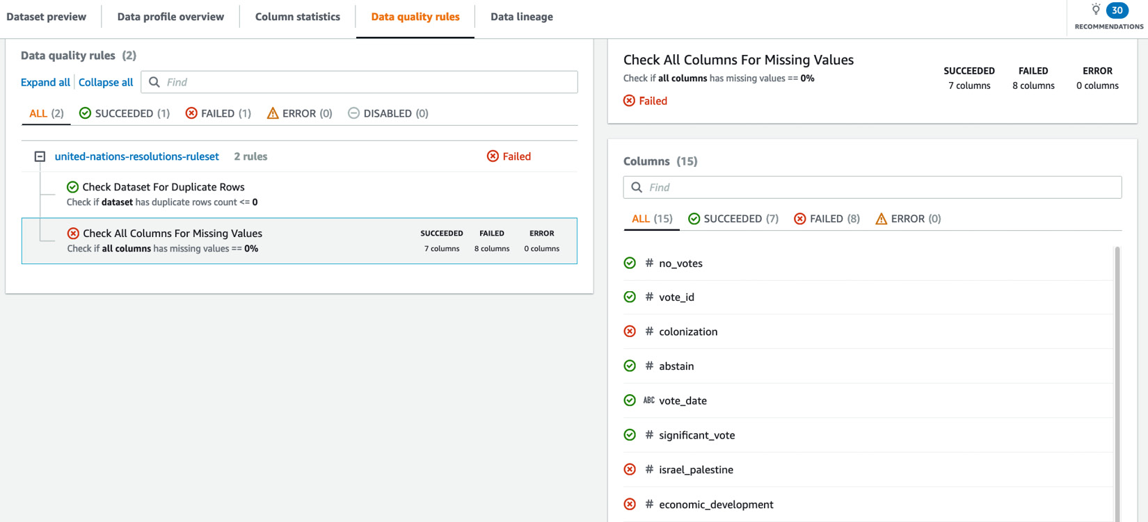
Figure 4.5 – Data profile generated based on user-defined DQ Rules
Using the insights generated by profile jobs, you can plan the data preparation steps according to your requirements and write the output to your destination data store. For instance, now that we know there are missing values in some of the columns, we can define transformations to handle those missing values – for example, populate with the last valid value, populate it with an empty string, or use a custom value.
Similarly, data masking transformations such as redaction, substitution, and hash functions can be applied to columns flagged as PII. We can even encrypt the data using probabilistic (using an AWS KMS key) or deterministic encryption (using a secret in AWS Secrets Manager) and decrypt the data when necessary.
There are over 250 transformations available in AWS Glue DataBrew for cleaning, reshaping, and preparing data based on the requirements and new transformations are being added to DataBrew frequently. A complete list of all the recipe steps and functions can be found in the AWS Glue DataBrew documentation at https://docs.aws.amazon.com/databrew/latest/dg/recipe-actions-reference.html.
Usage patterns for services/tools differ from one organization to another. An organization can choose to use AWS Glue DataBrew as its tool of choice for all data preparation workloads. However, if an organization prefers to use SQL or ETL scripts for their data preparation workload, AWS Glue DataBrew can be used for prototyping a data preparation pipeline. Then, data engineers can use the recipe in DataBrew as a reference to the authoring Glue ETL job. This allows other individuals within an organization who do not have Spark/Glue ETL programming skills to actively collaborate in data preparation workflows. Using this approach will reduce the effort and time taken by engineers to explore the data and design the data preparation steps from scratch.
Now that we know how we can leverage AWS Glue DataBrew for data preparation using a visual interface, let’s learn how to prepare data using a source code-based approach in AWS Glue.
Source code-based approach to data preparation using AWS Glue
While AWS Glue DataBrew offers a visual interface-based approach to tackle data preparation tasks in a data integration workflow, AWS Glue offers AWS Glue ETL and AWS Glue Studio as source code/SQL-based approaches for the same. AWS Glue ETL and AWS Glue Studio require us to have some level of Glue/Spark programming knowledge to implement ETL jobs, which aids in data preparation as we get a much higher level of flexibility compared to AWS Glue DataBrew. With AWS Glue DataBrew, we can use pre-built transformations to prepare data. Since there are no such restrictions in AWS Glue ETL and AWS Glue Studio, we can design and develop custom transformations based on our requirements using existing Glue/Spark ETL APIs and extensions.
AWS Glue ETL and AWS Glue Studio
In Chapter 2, Introduction to Important AWS Glue Features, and Chapter 3, Data Ingestion, we briefly discussed some of the features of AWS Glue ETL and how they aid in data ingestion. In this section, we will explore different features of AWS Glue ETL and AWS Glue Studio and how these can be leveraged to prepare data.
Based on our discussion in Chapter 2, Introduction to Important AWS Glue Features, we know that a DynamicRecord is a data structure in AWS Glue in which individual rows/records in the dataset are processed and that a DynamicFrame is a distributed collection of DynamicRecord objects. To use Glue ETL transformations, the dataset must be represented as a Glue DynamicFrame, not an Apache Spark DataFrame. We can author ETL scripts using several methods on AWS Glue Studio, Interactive Sessions, or even locally on our development workstation using our preferred IDE or text editor since AWS Glue runtime libraries are publicly available. You can refer to the AWS Glue documentation at https://docs.aws.amazon.com/glue/latest/dg/aws-glue-programming-etl-libraries.html to explore different ETL job development options.
AWS Glue Studio is a new visual interface that makes it easy to author, run, and monitor AWS Glue ETL Jobs. AWS Glue Studio enables us to design and develop ETL jobs using a visual editor (Figure 4.6), implement complex operations such as PII detection and redaction, provide interactive ETL script development using Jupyter notebooks, set up custom/marketplace connectors to connect to SaaS/custom data stores, and easily monitor ETL job runs using a unified monitoring dashboard:

Figure 4.6 – Visual job editor in AWS Glue Studio
In the next section, we’ll learn how to clean and prepare data using some of the transformations and extensions available in AWS Glue ETL.
Data transformation using AWS Glue ETL
Data preparation can be done in AWS Glue ETL by making use of built-in extensions and transformations. A complete list of extensions and transformations, syntax, and usage instructions can be found in the AWS Glue ETL documentation:
- AWS Glue Scala ETL jobs: https://docs.aws.amazon.com/glue/latest/dg/glue-etl-scala-apis.html
- AWS Glue PySpark ETL jobs: https://docs.aws.amazon.com/glue/latest/dg/aws-glue-programming-python.html
In this section, we will explore some of the most commonly used transformations in AWS Glue ETL.
ApplyMapping
The ApplyMapping transformation allows us to specify a declarative mapping of columns to a specified DynamicFrame. This transformation takes a DynamicFrame and a list of tuples, each consisting of the column name and data type mapping in the source and target DynamicFrames. This transformation is helpful when we want to rename columns or restructure a nested schema or change the data type of a column. It is important to specify a mapping for all the columns that are to be present in the target DynamicFrame. If a mapping is not defined for a column, that column will be dropped in the target DynamicFrame.
For example, let’s assume there’s a dataset with the following nested schema:
root
|-- email: string
|-- employee: struct
| |-- employee_id: int
| |-- employee_name: string
We can rename the email column employee_email and move the column under the employee struct using the following ApplyMapping transformation:
mappingList = [("email", "string", "employee.employee_email", "string"), ("employee.employee_id", "int", "employee.employee_id", "int"), ("employee.employee_name", "string", "employee.employee_name", "string")]applyMapping0 = ApplyMapping.apply(frame=datasource0, mappings=mappingList)
In the preceding snippet, mappingList is the list of mapping tuples being passed to the ApplyMapping transform. We can also see the mapping tuple that maps the email column to employee.employee_email. This mapping is essentially renaming the column employee_email and moving the column under the employee struct. Now, when we print the schema of the applyMapping0 DynamicFrame, we will see the following:
>>> applyMapping0.printSchema()
root
|-- employee: struct
| |-- employee_email: string
| |-- employee_id: int
| |-- employee_name: string
As you can see, by using the ApplyMapping transformation, we were able to achieve two things:
- Rename the column employee_email.
- Reshape the schema of the dataset to move the email column under the employee struct.
Now, let’s look at another commonly used transformation: Relationalize.
Relationalize
The Relationalize transform helps us reshape a nested schema of the dataset by flattening it. Any array columns that are present are pivoted out. This transformation is extremely helpful when we are working with a dataset that has a nested schema structure and we want to write the output to a relational database.
Let’s see this transformation in action. Let’s assume there is a dataset with the following schema. You will be able to find the source code and sample dataset for this example in this book’s GitHub repository at https://github.com/PacktPublishing/Serverless-ETL-and-Analytics-with-AWS-Glue/tree/main/Chapter04:
>>> datasource1.printSchema()
root
|-- company: string
|-- employees: array
| |-- element: struct
| | |-- email: string
| | |-- name: string
Now, let’s apply the Relationalize transformation to flatten this schema. In return, we will get a DynamicFrameCollection populated with DynamicFrames. Any array columns present in the dataset are pivoted out to a separate DynamicFrame:
relationalize0 = Relationalize.apply(frame=datasource1, staging_path='/tmp/glue_relationalize', name='company')
To list the keys for the different DynamicFrames that have been generated, we can use the keys() method on the returned DynamicFrameCollection. In the preceding example, that would be relationalize0:
>>> relationalize0.keys()
dict_keys(['company', 'company_employees'])
Now, since two DynamicFrames in DynamicFrameCollection were returned, it would be easier to interact with them separately if we extract them from DynamicFrameCollection. We could select() each of those DynamicFrames and use the show() method to see their contents. Alternatively, we can use the SelectFromCollection transformation to select individual DynamicFrames:
>>> company_Frame = relationalize0.select('company')>>> company_Frame.toDF().show()
+----------+---------+
| company|employees|
+----------+---------+
|DummyCorp1| 1|
|DummyCorp2| 2|
|DummyCorp3| 3|
+----------+---------+
>>> emp_Frame = relationalize0.select('company_employees')>>> emp_Frame.toDF().show()
+---+-----+-------------------+------------------+
| id|index|employees.val.email|employees.val.name|
+---+-----+-------------------+------------------+
| 1| 0| [email protected]| foo1|
| 1| 1| [email protected]| bar1|
| 2| 0| [email protected]| foo2|
| 2| 1| [email protected]| bar2|
| 3| 0| [email protected]| foo3|
| 3| 1| [email protected]| bar3|
+---+-----+-------------------+------------------+
As you may recall, the Relationalize transform has pivoted the employees column and created a new DynamicFrame with additional columns: id and index. The id column acts similarly to a foreign key for the employees column in the company DynamicFrame.
However, for us to be able to write the flattened data to a relational database, we need the data to be present in one DynamicFrame. To bring both of these DynamicFrames together, we can use the Join transform. Let’s look at the Join transform and see how it works.
Join
The Join transform, as its name suggests, joins two DynamicFrames. A Join transform in AWS Glue performs an equality join. If you are interested in performing other types of Join (for example, broadcast joins) in Glue ETL, you will have to convert the DynamicFrame into a Spark DataFrame.
Let’s continue with our example and join the two DynamicFrames that were created by Relationalize while using employees and id as the keys:
join0 = Join.apply(frame1 = company_Frame, frame2 = emp_Frame, keys1 = 'employees', keys2 = 'id')
Let’s use the show() function to see the joined data:
>>> join0.toDF().show(truncate=False)
This will result in the following output:

Figure 4.7 – Output demonstrating a Join transformation
As you can see, the email and name array columns have been renamed employees.val.email and employees.val.name, respectively. This is the result of pivoting the array in the Relationalize transformation. This can be corrected using the RenameField transformation before joining the DynamicFrames.
Now, let’s look at the RenameField transformation to see how we can rename columns.
RenameField
The RenameField transformation allows us to rename columns. This transformation takes three parameters as input – a DynamicFrame where the column needs to be renamed, the name of the column to be renamed, and the new name for the column.
In our example, we saw that after the array was pivoted by the Relationalize transform, the email and name array columns were renamed employees.val.email and employees.val.name, respectively. To rename the columns so that they have their original names, we can use the following code snippet:
renameField0 = RenameField.apply(frame = join0, old_name = "`employees.val.email`", new_name = "email")
renameField1 = RenameField.apply(frame = renameField0, old_name = "`employees.val.name`", new_name = "name")
You may have noticed the wrapping backquotes (`) for the old column names in the preceding code snippet. This is because we have a dot (.) character in the name of the column itself and here, the dot character does not represent a nested structure. To suppress the default behavior of the dot character, we have wrapped the column names in backquotes.
We can confirm that the columns have been successfully renamed by printing the schema of the renameField1 DynamicFrame. Now that we have a flattened schema structure and the columns have been renamed according to our requirements using transformations such as Relationalize, Join, and RenameField, we can safely write the resultant DynamicFrame to a table in a relational database.
Now, let’s look at some of the other transformations available in AWS Glue ETL.
Unbox
The Unbox transformation is helpful when a column in a dataset contains data in another format. Let’s assume that we are working with a dataset that’s been exported from a table in a relational database and that one of the columns has a JSON object stored as a string.
If we continue to use string data types for this JSON object, we won’t be able to analyze the data present in this column as easily as the downstream application may not know how to parse it. Even if it does, the queries would be extremely complex. Since the purpose of the data preparation step is to clean and reshape the data, it is much better to address this within the data preparation workflow.
Let’s assume that our dataset has the following schema:
root
|-- location: string
|-- companies_json: string
When we use the show() method on the DynamicFrame, we will see that there is a JSON string in the companies_json column:
+-----------+--------------------+
| location| companies_json|
+-----------+--------------------+
|Seattle, WA|{"jsonrecords":[{...|+-----------+--------------------+
Now, let’s see how the Unbox transform can help us unpack this JSON object and merge the schema of the JSON object with the DynamicFrame schema:
>>> unbox0 = Unbox.apply(frame = datasource2, path = "companies_json", format = "json")
>>> unbox0.printSchema()
root
|-- location: string
|-- companies_json: struct
| |-- jsonrecords: array
| | |-- element: struct
| | | |-- company: string
| | | |-- employees: array
| | | | |-- element: struct
| | | | | |-- email: string
| | | | | |-- name: string
As we can see, the schema from the JSON object was merged into DynamicFrame’s schema. Now, we can use other transformations to further transform the data or output the DynamicFrame as-is.
Now, there might be situations where you run into an issue when applying a transformation in Glue ETL and you may notice that some or all the records in a DynamicFrame have gone missing. This may happen if there was an error when parsing the records. How do we find out if this has happened? Well, AWS Glue ETL has a transformation that captures the nested error records called ErrorsAsDynamicFrame. Let’s take a look at how this works.
ErrorsAsDynamicFrame
This transformation takes a DynamicFrame as input and returns the nested error records that have been encountered up until the creation of the input DynamicFrame. In the Unbox transform example, we used a JSON string nested within a record to demonstrate the capabilities of Unbox. Let’s introduce a syntax error into the JSON string of one of the records by removing a curly brace or a comma that will interfere with the normal functioning of the JSON parser.
The following source code can be found in this book’s GitHub repository at https://github.com/PacktPublishing/Serverless-ETL-and-Analytics-with-AWS-Glue/tree/main/Chapter04:
# Refer GitHub repository for Sample code-gen function createSampleDynamicFrameForErrorsAsDynamicFrame()
>>> datasource2 = createSampleDynamicFrameForErrorsAsDynamicFrame()
>>> datasource2.toDF().show()
+-----------+--------------------+
| location| companies_json|
+-----------+--------------------+
|Seattle, WA|{"jsonrecords":[{...||Sydney, NSW|{"jsonrecords":[{...|+-----------+--------------------+
>>> unbox0 = Unbox.apply(frame = datasource2, path = "companies_json", format = "json")
>>> unbox0.toDF().show()
+-----------+--------------------+
| location| companies_json|
+-----------+--------------------+
|Seattle, WA|{[{DummyCorp1, [{...|+-----------+--------------------+
>>> ErrorsAsDynamicFrame.apply(unbox0).count()
1
>>> ErrorsAsDynamicFrame.apply(unbox0).toDF().show()
+--------------------+
| error|
+--------------------+
|{{ File "/tmp/66...|+--------------------+
As we can see, the valid JSON record that was in the DynamicFrame was parsed correctly by the parser. However, the invalid record was not parsed and we can see that the ErrorsAsDynamicFrame class has captured the errors. As part of the ETL script, we can have validation steps using this class to ensure there were no errors when transforming data.
You may have noticed by now that each of the AWS Glue ETL transforms have two parameters available. These parameters specify the error threshold for each transformation:
- stageThreshold specifies the maximum number of errors that can occur in a given transformation for which the job needs to fail.
- totalThreshold specifies the maximum number of errors up to and including the current transformation.
We can leverage these parameters to manage error handling behavior in AWS Glue ETL.
There are several other transformations available in AWS Glue ETL that make it easy to reshape and clean data based on our requirements. It would not be practical to discuss each of the transformations available in AWS Glue ETL here as the service has been constantly evolving since it was released and new transformations and extensions are being added by AWS. You can find an exhaustive list of transformations, syntax, and examples in the AWS Glue documentation, as mentioned at the beginning of this section.
Now that we are familiar with AWS Glue DataBrew, AWS Glue ETL, and AWS Glue Studio, it is important to know which tool/service to choose for your workload.
Selecting the right service/tool
In the previous sections, we looked at the different features, transformations, and extensions/APIs that are available in AWS Glue DataBrew, AWS Glue Studio, and AWS Glue ETL for preparing data. With all the choices available and the varying sets of features in each of these tools, how do we pick a tool/service for our use case? There is no hard and fast rule in selecting a tool/service and the choice depends on several factors that need to be considered based on the use case.
As discussed earlier in this chapter, AWS Glue DataBrew empowers data analysts and data scientists to prepare data without writing source code. AWS Glue ETL, on the other hand, has a higher learning curve and requires Python/Scala programming knowledge and a fundamental understanding of Apache Spark. So, if the individuals preparing the data are not skilled in AWS Glue/Spark ETL programming, they can use AWS Glue DataBrew.
One of the important factors to consider while choosing a tool/service is whether the data preparation tasks being planned can be implemented using the tool/service. While AWS Glue DataBrew has a library of over 250 pre-built transformations, they may still not cover some of the transformations required to implement your data preparation workflow or it might be too complex to implement your workflow using built-in transformations in DataBrew. In such cases, we can simplify the workflow by writing an ETL job in AWS Glue ETL since we have the flexibility to write custom transformations. We can leverage built-in AWS Glue ETL transformations or we can custom-design our transformations using Apache Spark APIs.
Another factor that can influence this decision is whether the data preparation workflow that’s being implemented is a one-off operation or something that needs to be accomplished quite frequently. If the data preparation tasks are simple and infrequent, it would not justify the effort involved in writing source code manually. In such cases, we can use AWS Glue DataBrew or AWS Glue Studio’s visual job editor to set up an ETL job to accomplish our tasks. However, if the tasks are complex, require a higher level of flexibility, and are going to be performed regularly, AWS Glue ETL would be a better choice as we can customize the ETL job based on our requirements.
To summarize, it is important to consider the use case and construct a plan based on the requirements. Some of the key considerations that could factor into the decision-making process are as follows:
- Features offered by a specific tool and whether our tasks can be accomplished using built-in transforms
- The skill sets of individuals within the team
- The complexity of the workflow that is being implemented
- The frequency of data preparation operations
So, it is important to consider the use case at hand, plan your data preparation workflow, and then choose a tool/service to implement your workflow. Otherwise, you could end up wasting a lot of time and effort in designing your workflow using a specific tool/service that was not fit for your use case to begin with.
Summary
In this chapter, we discussed the fundamental concepts and importance of data preparation within a data integration workflow. We explored how we can prepare data in AWS Glue using both visual interfaces and source code.
We explored different features of AWS Glue DataBrew and saw how we can implement profile jobs to profile the data and gather insights about the dataset being processed, as well as how to use a DQ Ruleset to enrich the data profile, use PII detection and redaction, and perform column encryption using deterministic and probabilistic encryption. We also discussed how we can apply transformations, build a recipe using those transformations, create a job using that recipe, and run the job.
Then, we discussed source code-based ETL development using AWS Glue ETL jobs and the different features of AWS Glue Studio before exploring some of the popular transformations and extensions available in AWS Glue ETL. We saw how these transformations can be used in specific use cases while covering source code examples and how we can detect and handle errors during data preparation in AWS Glue ETL.
We talked about different factors that need to be considered while choosing a service/tool in AWS Glue and the importance of considering the use case and planning while designing our data preparation workflow.
In the next chapter, we will discuss the importance of data layouts and how we can design data layouts to optimize analytics workloads. We will be exploring some of the concepts that factor into performance and resource consumption during query execution, such as data formats, compression, bucketing, partitioning, and compactions.