
The perceptron is a basic processing element that performs a binary classification by mapping a scalar or vector to a binary (or XOR) value {true, false} or {-1, +1}. The original perceptron algorithm was defined as a single layer of neurons for which each value xi of the feature vector is processed in parallel and generates a single output y. The perceptron was later extended to encompass the concept of an activation function.
The single layer perceptrons are limited to process a single linear combination of weights and input values. Scientists found out that adding intermediate layers between the input and output layers enable them to solve more complex classification problems. These intermediate layers are known as hidden layers because they interface only with other perceptrons. Hidden nodes can be accessed only through the input layer.
From now on, we will use a three-layered perceptron to investigate and illustrate the properties of neural networks, as shown here:

A three-layered perceptron
The three-layered perceptron requires two sets of weights: wij to process the output of the input layer to the hidden layer and vij between the hidden layer and the output layer. The intercept value w0, in both linear and logistic regression, is represented with +1 in the visualization of the neural network (w0.1+ w1.x1+w2.x2+ …).
Note
A FFNN without a hidden layer
A FFNN without a hidden layer is similar to a linear statistical model. The only transformation or connection between the input and output layer is actually a linear regression. A linear regression is a more efficient alternative to the FFNN without a hidden layer.
The description of the MLP components and their implementations rely on the following stages:
- An overview of the software design.
- A description of the MLP model components.
- The implementation of the four-step training cycle.
- The definition and implementation of the training strategy and the resulting classifier.
Note
Terminology
Artificial neural networks encompass a large variety of learning algorithms, the multilayer perceptron being one of them. Perceptrons are indeed components of a neural network organized as the input, output, and hidden layers. This chapter is dedicated to the multilayer perceptron with hidden layers. The terms "neural network" and "multilayer perceptron" are used interchangeably.
The perceptron is represented as a linear combination of weights wi and input values xi processed by the output unit activation function h, as shown here (M2):

The output activation function h has to be continuous and differentiable for a range of value of the weights. It takes different forms depending on the problems to be solved, as mentioned here:
- An identity for the output layer (linear formula) of the regression mode
- The sigmoid σ for hidden layers and output layers of the binomial classifier
- Softmax for the multinomial classification
- The hyperbolic tangent, tanh, for the classification using zero mean
The softmax formula is described in Step 1 – input forward propagation under Training epoch.
The output layers and hidden layers have a computational capability (dot product of weights, inputs, and activation functions). The input layer does not transform data. An n-layer neural network is a network with n computational layers. Its architecture consists of the following components:
- one input layer
- n-1 hidden layer
- one output layer
A fully connected neural network has all its input nodes connected to hidden layer neurons. Networks are characterized as partially connected neural networks if one or more of their input variables are not processed. This chapter deals with a fully connected neural network.
The structure of the output layer is highly dependent on the type of problems (regression or classification) you need to solve, also known as the operating mode of the multilayer perceptron. The type of problem at hand defines the number of output nodes [9:5]. Consider the following examples:
- A one-variate regression has one output node whose value is a real number [0, 1]
- A multivariate regression with n variables has n real output nodes
- A binary classification has one binary output node {0, 1} or {-1, +1}
- A multinomial or K-class classification has K binary output nodes
The implementation of the MLP classifier follows the same pattern as previous classifiers (refer to the Design template for immutable classifiers section in the Appendix A, Basic Concepts):
- An
MLPNetworkconnectionist network is composed of a layer of neurons of theMLPLayertype, connected by synapses of theMLPSynapsetype contained by a connector of theMLPConnectiontype. - All of the configuration parameters are encapsulated into a single
MLPConfigconfiguration class. - A model,
MLPModel, consists of a sequence of connection synapses. - The
MLPmultilayer perceptron class is implemented as a data transformation,ITransform, for which the model is automatically extracted from a training set with labels. - The
MLPmultilayer perceptron class takes four parameters: a configuration, a features set or time series of theXVSeriestype, a labeled dataset of theXVSeriestype, and an activation function of theFunction1[Double, Double]type.
The software components of the multilayer perceptron are described in the following UML class diagram:
.
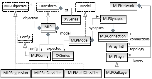
A UML class diagram for the multilayer perceptron
The class diagram is a convenient navigation map used to understand the role and relation of the Scala classes used to build an MLP. Let's start with the implementation of the MLP network and its components. The UML diagram omits the helper traits or classes such as Monitor or the Apache Commons Math components.
The MLPConfig configuration of the multilayer perceptron consists of the definition of the network configuration with its hidden layers, the learning and training parameters, and the activation function:
case class MLPConfig(
    val alpha: Double,  //1
    val eta: Double,
    val numEpochs: Int,
    val eps: Double,
    val activation: Double => Double) extends Config {  //1
}
For the sake of readability, the name of the configuration parameters matches the symbols defined in the mathematical formulation (line 1):
alpha: This is the momentum factor α that smoothes the computation of the gradient of the weights for online training. The momentum factor is used in the mathematical expression M10 in Step 2 – error backpropagation under Training epoch.eta: This is the learning rate η used in the gradient descent. The gradient descent updates the weights or parameters of a model by the quantity, eta.(predicted – expected).input, as described in the mathematical formulation M9 in Step 2 – error backpropagation section under The training epoch. The gradient descent was introduced in Let's kick the tires in Chapter 1, Getting Started.numEpochs: This is the maximum number of epochs (or cycles or episodes) allowed for training the neural network. An epoch is the execution of the error backpropagation across the entire observation set.eps: This is the convergence criteria used as an exit condition for the training of the neural network when error < eps.activation: This is the activation function used for nonlinear regression applied to hidden layers. The default function is the sigmoid (or the hyperbolic tangent) introduced for the logistic regression (refer to the Logistic function section in Chapter 6, Regression and Regularization).
The training and classification of an MLP model relies on the network architecture. The MLPNetwork class is responsible for creating and managing the different components and the topology of the network, that is layers, synapses, and connections.
The instantiation of the MLPNetwork class requires a minimum set of two parameters with an instance of the model as an optional third argument (line 2):
- An MLP execution configuration,
config, introduced in the previous section - A
topologydefined as an array of the number of nodes for each layer: input, hidden, and output layers. - A
modelwith theOption[MLPModel]type if it has already been generated through training, orNoneotherwise - An implicit reference to the operating
modeof the MLP
The code is as follows:
class MLPNetwork(config: MLPConfig,
     topology: Array[Int],
     model: Option[MLPModel] = None)
     (implicit mode: MLPMode){ //2

  val layers = topology.zipWithIndex.map { case(t, n) =>
    if(topology.size != n+1)
       MLPLayer(n, t+1, config.activation)
   else MLPOutLayer(n, t)
  }  //3
  val connections = zipWithShift1(layers,1).map{case(src,dst) =>
     new MLPConnection(config, src, dst,  model)} //4

  def trainEpoch(x: DblArray, y: DblArray): Double //5
  def getModel: MLPModel  //6
  def predict(x: DblArray): DblArray  //7
}
A MLP network has the following components, which are derived from the topology array:
- Multiple
layersof theMLPLayersclass (line3) - Multiple
connectionsof theMLPConnectionclass (line4)
The topology is defined as an array of number of nodes per layer, starting with the input nodes. The array indices follow the forward path within the network. The size of the input layer is automatically generated from the observations as the size of the features vector. The size of the output layer is automatically extracted from the size of the output vector (line 3).
The constructor for MLPNetwork creates a sequence of layers by assigning and ordering an MLPLayer instance to each entry in the topology (line 3). The constructor creates number of layers – 1 interlayer connections of the MLPConnection type (line 4). The zipWithShift1 method of the XTSeries object zips a time series with its duplicated shift by one element.
The trainEpoch method (line 5) implements the training of this network for a single pass of the entire set of observations (refer to the Putting it all together section under The training epoch). The getModel method retrieves the model (synapses) generated through training of the MLP (line 6). The predict method computes the output value generated from the network using the forward propagation algorithm (line 7).
The following diagram visualizes the interaction between the different components of a model: MLPLayer, MLPConnection, and MLPSynapse:

Core components of the MLP Network
First, let's start with the definition of the MLPLayer layer class, which is completely specified by its position (or rank) id in the network and the number of nodes, numNodes, it contains:
class MLPLayer(val id: Int, val numNodes: Int,
    val activation: Double => Double)  //8
    (implicit mode: MLPMode){  //9

  val output = Array.fill(numNodes)(1.0)  //10

  def setOutput(xt: DblArray): Unit =
      xt.copyToArray(output, 1) //11
  def activate(x: Double): Double = activation(x) .//12
  def delta(loss: DblArray, srcOut: DblArray,
      synapses: MLPConnSynapses): Delta //13
  def setInput(_x: DblArray): Unit  //14
}
The id parameter is the order of the layer (0 for input, 1 for the first hidden layer, and n – 1 for the output layer) in the network. The numNodes value is the number of elements or nodes, including the bias element, in this layer. The activation function is the last argument of the layer given a user-defined mode or objective (line 8). The operating mode has to be provided implicitly prior to the instantiation of a layer (line 9).
The output vector for the layer is an uninitialized array of values updated during the forward propagation. It initializes the bias value with the value 1.0 (line 9). The matrix of difference of weights, deltaMatrix, associated with the output vector (line 10) is updated using the error backpropagation algorithm, as described in the Step 2 – error back propagation section under The training epoch. The setOutput method initializes the output values for the output and hidden layers during the backpropagation of the error on the output of the network (expected – predicted) values (line 11).
The activate method invokes the activation method (tanh, sigmoid, …) defined in the configuration (line 12).
The delta method computes the correction to be applied to each weight or synapses, as described in the Step 2 – error back propagation section under The training epoch (line 13).
The setInput method initializes the output values for the nodes of the input and hidden layers, except the bias element, with the value x (line 14). The method is invoked during the forward propagation of input values:
def setInput(x: DblVector): Unit =
  x.copyToArray(output, output.length -x.length)
The methods of the MLPLayer class for the input and hidden layers are overridden for the output layer of the MLPOutLayer type.
Contrary to the hidden layers, the output layer does not have either an activation function or a bias element. The MLPOutLayer class has the following arguments: the order id in the network (as the last layer of the network) and the number, numNodes, of the output or nodes (line 15):
class MLPOutLayer(id: Int, numNodes: Int)
    (implicit mode: MLP.MLPMode)  //15
  extends MLPLayer(id, numNodes, (x: Double) => x) {

  override def numNonBias: Int = numNodes
  override def setOutput(xt: DblArray): Unit =
    obj(xt).copyToArray(output)
  override def delta(loss: DblArray, srcOut: DblArray,
     synapses: MLPConnSynapses): Delta
 …
}
The numNonBias method returns the actual number of output values from the network. The implementation of the delta method is described in the Step 2 – error back propagation section under The training epoch.
A synapse is defined as a pair of real (a floating point) values:
- The weight wij of the connection from the neuron i of the previous layer to the neuron j
- The weights' adjustment (or gradient of weights) ∆wij
Its type is defined as MLPSynapse, as shown here:
type MLPSynapse = (Double, Double)The connections are instantiated by selecting two consecutive layers of an index n (with respect to n + 1) as a source (with respect to destination). A connection between two consecutive layers implements the matrix of synapses as the (wij
, ∆wij) pairs. The MLPConnection instance is created with the following parameters (line 16):
- Configuration parameters,
config - The source layer, sometimes known as the ingress layer,
src - The
dstdestination (or egress) layer - A reference to the
modelif it has already been generated through training orNoneif the model has not been trained - An implicitly defined operating
modeor objectivemode
The MLPConnection class is defined as follows:
type MLPConnSynapses = Array[Array[MLPSynapse]]

class MLPConnection(config: MLPConfig,
    src: MLPLayer,
    dst: MLPLayer,
    model: Option[MLPModel]) //16
    (implicit mode: MLP.MLPMode) {

  var synapses: MLPConnSynapses  //17
  def connectionForwardPropagation: Unit //18
  def connectionBackpropagation(delta: Delta): Delta  //19
    …
}
The last step in the initialization of the MLP algorithm is the selection of the initial (usually random) values of the weights (synapse) (line 17).
The MLPConnection methods implement the forward propagation of weights' computation for this connectionForwardPropagation connection (line 18) and the backward propagation of the delta error during training connectionBackpropagation (line 19). These methods are described in the next section related to the training of the MLP model.
The initialization values for the weights depends is domain specific. Some problems require a very small range, less than 1e-3, while others use the probability space [0, 1]. The initial values have an impact on the number of epochs required to converge toward an optimal set of weights [9:6].
Our implementation relies on the sigmoid activation function and uses the range [0, BETA/sqrt(numOutputs + 1)] (line 20). However, the user can select a different range for random values, such as [-r, +r] for the tanh activation function. The weight of the bias is obviously defined as w0
=+1, and its weight adjustment is initialized as ∆w0 = 0, as shown here (line 20):
var synapses: MLPConnSynapses = if(model == None) {
  val max = BETA/Math.sqrt(src.output.length+1.0) //20
  Array.fill(dst.numNonBias)(
    Array.fill(src.numNodes)((Random.nextDouble*max,0.00))
  )
} else model.get.synapses(src.id)  //21
The connection derives its weights or synapses from a model (line 21) if it has already been created through training.
The MLPNetwork class defines the topological model of the multilayer perceptron. The weights or synapses are the attributes of the model of the MLPModel type generated through training:
case class MLPModel(
   val synapses: Vector[MLPConnSynapses]) extends Model
The model can be stored in a simple key-value pair JSON, CVS, or sequence file.
Note
Encapsulation and the model factory
The network components: connections, layers, and synapses are implemented as top-level classes for the sake of clarity. However, there is no need for the model to expose its inner workings to the client code. These components should be declared as an inner class to the model. A factory design pattern would be perfectly appropriate to instantiate an MLPNetwork instance dynamically [9:7].
Once initialized, the MLP model is ready to be trained using a combination of forward propagation, output error back propagation, and iterative adjustment of weights and gradients of weights.
There are three distinct types of problems or operating modes associated with the multilayer perceptron:
- The binomial classification (binary) with two classes and one output
- The multinomial classification (multiclass) with n classes and output
- Regression
Each operating mode has distinctive error, hidden layer, and output layer activation functions, as illustrated in the following table:
|
Operating modes |
Error function |
Hidden layer activation function |
Output layer activation function |
|---|---|---|---|
|
Binomial classification |
Cross-entropy |
Sigmoid |
Sigmoid |
|
Multinomial classification |
Sum of squares error or mean squared error |
Sigmoid |
Softmax |
|
Regression |
Sum of squares error or mean squared error |
Sigmoid |
Linear |
A table for operating modes of the multilayer perceptron
The cross-entropy is described by the mathematical expressions M6 and M7 and the softmax uses the formula M8 in the Step 1 – input forward propagation section under The training epoch.
One important issue is to find a strategy to conduct the training of a time series as an ordered sequence of data. There are two strategies to create an MLP model for a time series:
- Batch training: The entire time series is processed at once as a single input to the neural network. The weights (synapses) are updated at each epoch using the sum of the squared errors on the output of the time series. The training exits once the sum of the squared errors meets the convergence criteria.
- Online training: The observations are fed to the neural network one at a time. Once the time series has been processed, the total of the sum of the squared errors (
sse) for the time series for all the observations are computed. If the exit condition is not met, the observations are reprocessed by the network.
An illustration on online and batch training
An online training is faster than batch training because the convergence criterion has to be met for each data point, possibly resulting in a smaller number of epochs [9:12]. Techniques such as the momentum factor, which is described earlier, or any adaptive learning scheme improves the performance and accuracy of the online training methodology.
The online training strategy is applied to all the test cases of this chapter.
The training of the model processes the training observations iteratively multiple times. A training cycle or iteration is known as an epoch. The order of observations is shuffled for each epoch. The three steps of the training cycle are as follows:
- Forward the propagation of the input value for a specific epoch.
- Computation and backpropagation of the output error.
- Evaluate the convergence criteria and exit if the criteria is met.
The computation of the network weights during training can use the difference between labeled data and actual output for each layer. But this solution is not feasible because the output of the hidden layers is actually unknown. The solution is to propagate the error on the output values (predicted values) backward to the input layer through the hidden layers, if an error is defined.
The three steps of the training cycle or training epoch are summarized in the following diagram:

An iterative implementation of the training for MLP
Let's apply the three steps of a training epoch in the trainEpoch method of the MLPNetwork class using a simple foreach Scala higher order function, as shown here:
def trainEpoch(x: DblArray, y: DblArray): Double = {
  layers.head.setInput(x)  //22
  connections.foreach( _.connectionForwardPropagation) //23

  val err = mode.error(y, layers.last.output)
  val bckIterator = connections.reverseIterator

  var delta = Delta(zipToArray(y, layers.last.output)(diff)) //24
  bckIterator.foreach( iter =>
     delta = iter.connectionBackpropagation(delta))  //25
  err  //26
}
You can certainly recognize the first two stages of the training cycle: the forward propagation of the input and the backpropagation of the error of the online training of a single epoch.
The execution of the training of the network for one epoch, trainEpoch, initializes the input layer with observations, x (line 22). The input values are propagated through the network by invoking connectionForwardPropagation for each connection (line 23). The delta error is initialized from the values in the output layer and the expected values, y (line 24).
The training method iterates through the connections backward to propagate the error through each connection by invoking the connectionBackpropagation method on the backward iterator, bckIterator (line 25). Finally, the training method returns the cumulative error, mean square error, or cross entropy, according to the operating mode (line 26).
This approach is not that different than the beta (or backward) pass in the hidden Markov model, which was covered in the Beta – the backward pass section in Chapter 7, Sequential Data Models.
Let's take a look at the implementation of the forward and backward propagation algorithm for each type of connection:
- An input or hidden layer to a hidden layer
- A hidden layer to an output layer
As mentioned earlier, the output values of a hidden layer are computed as the sigmoid or hyperbolic tangent of the dot product of the weights wij and the input values xi.
In the following diagram, the MLP algorithm computes the linear product of the weights wij and input xi for the hidden layer. The product is then processed by the activation function σ (the sigmoid or hyperbolic tangent). The output values zj are then combined with the weights vij of the output layer that doesn't have an activation function:
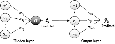
The distribution of weights in MLP hidden and output layers
The mathematical formulation of the output of a neuron j is defined as a composition of the activation function and the dot product of the weights wij and input values xi.


As seen in the network architecture section, the output values for the multinomial (or multiclass) classification with more than two classes are normalized using an exponential function, as described in the following Softmax section.
The computation of the output values y from the input x is known as the input forward propagation. For the sake of simplicity, we represent the forward propagation between layers with the following block diagram:

A computation model of the input forward propagation
The preceding diagram conveniently illustrates a computational model for the input forward propagation, as the programmatic relation between the source and destination layers and their connectivity. The input x is propagated forward through each connection.
The connectionForwardPropagation method computes the dot product of the weights and the input values and applies the activation function, in the case of hidden layers, for each connection. Therefore, it is a member of the MLPConnection class.
The forward propagation of input values across the entire network is managed by the MLP algorithm itself. The forward propagation of the input value is used in the classification or prediction y = f(x). It depends on the value weights wij and vij that need to be estimated through training. As you may have guessed, the weights define the model of a neural network similar to the regression models. Let's take a look at the connectionForwardPropagation method of the MLPConnection class:
def connectionForwardPropagation: Unit = {
  val _output = synapses.map(x => {
    val dot = inner(src.output, x.map(_._1) ) //27
    dst.activate(dot)  //28
  })
  dst.setOutput(_output) //29
}
The first step is to compute the linear inner (or dot) product (refer to the Time series in Scala section in Chapter 3, Data Preprocessing) of the output, _output, of the current source layer for this connection and the synapses (weights) (line 27). The activation function is computed by applying the activate method of the destination layer to the dot product (line 28). Finally, the computed value, _output, is used to initialize the output for the destination layer (line 29).
As mentioned in the Problem types (modes) section, there are two approaches to compute the error or loss on the output values:
- The sum of the squared errors between expected and predicted output values, as defined in the M5 mathematical expression
- Cross-entropy of expected and predicted values described in the M6 and M7 mathematical formulas


The sum of squared errors and mean squared error functions have been described in the Time series in Scala section in Chapter 3, Data Preprocessing.
The crossEntropy method of the XTSeries object for a single variable is implemented as follows:
def crossEntropy(x: Double, y: Double): Double =
  -(x*Math.log(y) + (1.0 - x)*Math.log(1.0 - y))
The computation of the cross entropy for multiple variable features as a signature is similar to the single variable case:
def crossEntropy(xt: DblArray, yt: DblArray): Double =
  yt.zip(xt).aggregate(0.0)({ case (s, (y, x)) =>
s - y*Math.log(x)}, _ + _)In the network architecture section, you learned that the structure of the output layer depends on the type of problems that need to be resolved, also known as operating modes. Let's encapsulate the different operating modes (binomial, multinomial classification, and regression) into a class hierarchy, implementing the MLPMode trait. The MLPMode trait has two methods that is specific to the type of the problem:
apply: This is the transformation applied to the output valueserror: This is the computation of the cumulative error for the entire observation set
The code will be as follows:
trait MLPMode {
  def apply(output: DblArray): DblArray   //30
  def error(labels: DblArray, output: DblArray): Double =
    mse(labels, output)  //31
}
The apply method applies a transformation to the output layer, as described in the last column of the operating modes table (line 30). The error function computes the cumulative error or loss in the output layer for all the observations, as described in the first column of the operating modes table (line 31).
The transformation in the output layer of the MLPBinClassifier binomial (two-class) classifier consists of applying the sigmoid function to each output value (line 32). The cumulative error is computed as the cross entropy of the expected output, labels, and the predicted output (line 33):
class MLPBinClassifier extends MLPMode {
  override def apply(output: DblArray): DblArray =
    output.map(sigmoid(_))  //32
  override def error(labels: DblArray,
      output: DblArray): Double =
    crossEntropy(labels.head, output.head)  //33
}
The regression mode for the multilayer perceptron is defined according to the operating modes table in the Problem types (modes) section:
class MLPRegression extends MLPMode  {
  override def apply(output: DblArray): DblArray = output
}
The multinomial classifier mode is defined by the MLPMultiClassifier class. It uses the softmax method to boost the output with the highest value, as shown in the following code:
class MLPMultiClassifier extends MLPMode {
  override def apply(output: DblArray):DblArray = softmax(output)
}
The softmax method is applied to the actual output value, not the bias. Therefore, the first node y(0) = +1 has to be dropped before applying the softmax normalization.
In the case of a classification problem with K classes (K > 2), the output has to be converted into a probability [0, 1]. For problems that require a large number of classes, there is a need to boost the output yk with the highest value (or probability). This process is known as exponential normalization or softmax [9:8].
Here is the simple implementation of the softmax method of the MLPMultiClassifier class:
def softmax(y: DblArray): DblArray = {
  val softmaxValues = new DblArray(y.size)
  val expY = y.map( Math.exp(_))  //34
  val expYSum = expY.sum  //35

  expY.map( _ /expYSum).copyToArray(softmaxValues, 1) //36
  softmaxValues
}
The softmax method implements the M8 mathematical expression. First, the method computes the expY exponential values of the output values (line 34). The exponentially transformed outputs are then normalized by their sum, expYSum, (line 35) to generate the array of the softmaxValues output (line 36). Once again, there is no need to update the bias element y(0).
The second step in the training phase is to define and initialize the matrix of delta error values to be back propagated between layers from the output layer back to the input layer.
The error backpropagation is an algorithm that estimates the error for the hidden layer in order to compute the change in weights of the network. It takes the sum of squared errors of the output as the input.
Note
The convention for computing the cumulative error
Some authors refer to the backpropagation as a training methodology for an MLP, which applies the gradient descent to the output error defined as either the sum of squared errors, or the mean squared error for multinomial classification or regression. In this chapter, we keep the narrower definition of the backpropagation as the backward computation of the sum of squared errors.
The connection weights ∆v and ∆w are adjusted by computing the sum of the derivatives of the error, over the weights scaled with a learning factor. The gradient of weights are then used to compute the error of the output of the source layer [9:9].
The simplest algorithm to update the weights is the gradient descent [9:10]. The batch gradient descent was introduced in Let's kick the tires in Chapter 1, Getting Started.
The gradient descent is a very simple and robust algorithm. However, it can be slower in converging toward a global minimum than the conjugate gradient or the quasi-Newton method (refer to the Summary of optimization techniques section in the Appendix A, Basic Concepts).
There are several methods available to speed up the convergence of the gradient descent toward a minimum, such as the momentum factor and adaptive learning coefficient [9:11].
Large variations of the weights during training increase the number of epochs required for the model (connection weights) to converge. This is particularly true for a training strategy known as online training. The training strategies are discussed in the next section. The momentum factor α is used for the remaining section of the chapter.
The simplest version of the gradient descent algorithm (M9) is selected by simply setting the momentum factor α to zero in the generic (M10) mathematical expression.
The objective of the training of a perceptron is to minimize the loss or cumulative error for all the input observations as either the sum of squared errors or the cross entropy as computed at the output layer. The error εk for each output neuron yk is computed as the difference between a predicted output value and label output value. The error cannot be computed on output values of the hidden layers zj because the label values for those layers are unknown:

An illustration of the back-propagation algorithm
In the case of the sum of squared errors, the partial derivative of the cumulative error over each weight of the output layer is computed as the composition of the derivative of the square function and the derivative of the dot product of weights and the input z.
As mentioned earlier, the computation of the partial derivative of the error over the weights of the hidden layer is a bit tricky. Fortunately, the mathematical expression for the partial derivative can be written as the product of three partial derivatives:
- The derivative of the cumulative error ε over the output value yk
- The derivative of the output value yk over the hidden value zj, knowing that the derivative of a sigmoid σ is σ(1 - σ)
- The derivative of the output of the hidden layer zj over the weights wij
The decomposition of the partial derivative produces the following formulas for updating the synapses' weights for the output and hidden neurons by propagating the error (or loss) ε.
Note
Output weights' adjustment
M11: The computation of delta δ and weight adjustment ∆v for the output layer with the predicted value ~y and expected value y, and output z of the hidden layer is as follows:
Hidden weights' adjustment
M12: The computation of delta δ and weight adjustment ∆w for the hidden layer with the predicted value ~y and expected value y, output z of the hidden layer, and the input value x is as follows:

The matrix δij is defined by the delta matrix in the Delta class. It contains the basic parameters to be passed between layers, traversing the network from the output layer back to the input layer. The parameters are as follows:
- Initial
lossor error computed at the output layer - Matrix of the
deltavalues from the current connection - Weights or
synapsesof the downstream connection (or connection between the destination layer and the following layer)
The code will be as follows:
case class Delta(val loss: DblArray,
  val delta: DblMatrix = Array.empty[DblArray],
  val synapses: MLPConnSynapses = Array.empty[Array[MLPSynapse]] )
The first instance of the Delta class is generated for the output layer using the expected values y, then propagated to the preceding hidden layer in the MLPNetwork.trainEpoch method (line 24):
val diff = (x: Double, y: Double) => x - y
Delta(zipToArray(y, layers.last.output)(diff))
The M11 mathematical expression is implemented by the delta method of the MLPOutLayer class:
def delta(error: DblArray, srcOut: DblArray,
     synapses: MLPConnSynapses): Delta = {

  val deltaMatrix = new ArrayBuffer[DblArray] //34
  val deltaValues = error./:(deltaMatrix)( (m, l) => {
    m.append( srcOut.map( _*l) )
    m
  })   //35
  new Delta(error, deltaValues.toArray, synapses)  //36
}
The method generates the matrix of delta values associated with the output layer (line 34). The M11 formula is actually implemented by the fold over the srcOut output value (line 35). The new delta instances are returned to the trainEpoch method of MLPNetwork and backpropagated to the preceding hidden layer (line 36).
The delta method of the MLPLayer class implements the M12 mathematical expression:
def delta(oldDelta: DblArray, srcOut: DblArray,
     synapses: MLPConnSynapses): Delta = {

  val deltaMatrix = new ArrayBuffer[(Double, DblArray)]
  val weights = synapses.map(_.map(_._1))
       .transpose.drop(1) //37

  val deltaValues = output.drop(1)
   .zipWithIndex./:(deltaMatrix){  // 38
     case (m, (zh, n)) => {
       val newDelta = inner(oldDelta, weights(n))*zh*(1.0 - zh)
       m.append((newDelta, srcOut.map( _ * newdelta) )
       m
     }
  }.unzip
  new Delta(deltaValues._1.toArray, deltaValues._2.toArray)//39
}
The implementation of the delta method is similar to the MLPOutLayer.delta method. It extracts the weights v from the output layer through transposition (line 37). The values of the delta matrix in the hidden connection is computed by applying the M12 formula (line 38). The new delta instance is returned to the trainEpoch method (line 39) to be propagated to the preceding hidden layer if one exists.
The computational model for the error backpropagation algorithm is very similar to the forward propagation of the input. The main difference is that the propagation of δ (delta) is performed from the output layer to the input layer. The following diagram illustrates the computational model of the backpropagation in the case of two hidden layers zs and zt:

An illustration of the backpropagation of the delta error
The connectionBackPropagation method propagates the error back from the output layer or one of the hidden layers to the preceding layer. It is a member of the MLPConnection class. The backpropagation of the output error across the entire network is managed by the MLP class.
It implements the two set of equations where synapses(j)(i)._1 are the weights wji, dst.delta is the vector of the error derivative in the destination layer, and src.delta is the error derivative of the output in the source layer, as shown here:
def connectionBackpropagation(delta: Delta): Delta = {  //40
  val inSynapses =  //41
    if( delta.synapses.length > 0) delta.synapses
    else synapses

  val delta = dst.delta(delta.loss, src.output,inSynapses) //42
  synapse = synapses.zipWithIndex.map{ //43
    case (synapsesj, j) => synapsesj.zipWithIndex.map{
      case ((w, dw), i) => {
        val ndw = config.eta*connectionDelta.delta(j)(i)
        (w + ndw - config.alpha*dw, ndw)
      }
    }
  }
  new Delta(connectionDelta.loss,
       connectionDelta.delta, synapses)
}
The connectionBackPropagation method takes delta associated with the destination (output) layer as an argument (line 40). The output layer is the last layer of the network, and therefore, the synapses for the following connection is defined as an empty matrix of length zero (line 41). The method computes the new delta matrix for the hidden layer using the delta.loss error and output from the source layer, src.output (line 42). The weights (synapses) are updated using the gradient descent with the momentum factor as in the M10 mathematical expression (line 43).
The convergence criterion consists of evaluating the cumulative error (or loss) relevant to the operating mode (or problem) against a predefined eps convergence. The cumulative error is computed using either the sum of squares error formula (M5) or the cross-entropy formula (M6 and M7). An alternative approach is to compute the difference of the cumulative error between two consecutive epochs and apply the eps convergence criteria as the exit condition.
The MLP class is defined as a data transformation of the ITransform type using a model implicitly generated from a training set, xt, as described in the Monadic data transformation section in Chapter 2, Hello World! (line 44).
The MLP algorithm takes the following parameters:
config: This is the configuration of the algorithmhidden: This is an array of the size of the hidden layers if anyxt: This is the time series of features used to train the modelexpected: This is the labeled output values for training purposemode: This is the implicit operating mode or objective of the algorithmf: This is the implicit conversion from feature from typeTtoDouble
The V type of the output of the prediction or classification method |> of this implicit transform is DblArray (line 45):
class MLP[T <: AnyVal](config: MLPConfig,
    hidden: Array[Int] = Array.empty[Int],
    xt: XVSeries[T],
    expected: XVSeries[T])
    (implicit mode: MLPMode, f: T => Double)
  extends ITransform[Array[T]](xt) with Monitor[Double] {  //44

  type V = DblArray  //45

  lazy val topology = if(hidden.length ==0)
    Array[Int](xt.head.size, expected.head.size)
  else  Array[Int](xt.head.size) ++ hidden ++
         Array[Int](expected.head.size)  //46

  val model: Option[MLPModel] = train
  def train: Option[MLPModel]   //47
  override def |> : PartialFunction[Array[T], Try[V]]
}
The topology is created from the xt input variables, the expected values, and the configuration of hidden layers, if any (line 46). The generation of the topology from parameters of the MLPNetwork class is illustrated in the following diagram:

Topology encoding for multi-layer perceptrons
For instance, the topology of a neural network with three input variables: one output variable and two hidden layers of three neurons each is specified as Array[Int](4, 3, 3, 1). The model is generated through training by invoking the train method (line 47). Finally, the |> operator of the ITransform trait is used for classification, prediction, or regression, depending on the selected operating mode (line 48).
Once the training cycle or epoch is defined, it is merely a matter of defining and implementing a strategy to create a model using a sequence of data or time series.
There are two approaches to find the most appropriate network architecture for a given classification or regression problem, which are follows:
- Destructive tuning: Starting with a large network, and then removing nodes, synapses, and hidden layers that have no impact on the sum of squared errors
- Constructive tuning: Starting with a small network, and then incrementally adding the nodes, synapses, and hidden layers that reduce the output error
The destructive tuning strategy removes the synapses by zeroing out their weights. This is commonly accomplished using regularization.
You have seen that regularization is a powerful technique to address overfitting in the case of the linear and logistic regression in the Ridge regression section in Chapter 6, Regression and Regularization. Neural networks can benefit from adding a regularization term to the sum of squared errors. The larger the regularization factor is, the more likely some weights will be reduced to zero, thus reducing the scale of the network [9:13].
The MLPModel instance is created (trained) during the instantiation of the multilayer perceptron. The constructor iterates through the training cycles (or epochs) over all the data points of the xt time series, until the cumulative is smaller than the eps convergence criteria, as shown in the following code:
def train: Option[MLPModel] = {
  val network = new MLPNetwork(config, topology) //48
  val zi =  xt.toVector.zip(expected.view)   // 49

  Range(0, config.numEpochs).find( n => {  //50
    val cumulErr = fisherYates(xt.size)
       .map(zi(_))
       .map{ case(x, e) => network.trainEpoch(x, e)}
       .sum/st.size   //51
     cumulErr  < config.eps  //52
  }).map(_ => network.getModel)
}
The train method instantiates an MLP network using the configuration and topology as the input (line 48). The method executes multiple epochs until either the gradient descent with a momentum converges or the maximum number of allowed iterations is reached (line 50). At each epoch, the method shuffles the input values and labels using the Fisher-Yates algorithm, invokes the MLPNetwork.trainEpoch method, and computes the cumulErr cumulative error (line 51). This particular implementation compares the value of the cumulative error against the eps convergence criteria as the exit condition (line 52).
Lazy views are used to reduce the unnecessary creation of objects (line 49).
Note
The exit condition
In this implementation, the training initializes the model as None if it does not converge before the maximum number of epochs are reached. An alternative would be to generate a model even in the case of nonconvergence and add an accuracy metric to the model, as in our implementation of the support vector machine (refer to the Training section under Support vector classifiers – SVC in Chapter 8, Kernel Models and Support Vector Machines).
Once the model is created during the instantiation of the multilayer perceptron, it is available to predict or classify the class of a new observation.
The Step 5 – implementing the classifier section under Let's kick the tires in Chapter 1, Getting Started, describes a home grown shuffling algorithm as an alternative to the scala.util.Random.shuffle method of the Scala standard library. This section describes an alternative shuffling mechanism known as the Fisher-Yates shuffling algorithm:
def fisherYates(n: Int): IndexedSeq[Int] = {

   def fisherYates(seq: Seq[Int]): IndexedSeq[Int] = {
     Random.setSeed(System.currentTimeMillis)
    (0 until seq.size).map(i => {
       var randomIdx: Int = i + Random.nextInt(seq.size-i) //53
       seq(randomIdx) ^= seq(i)    //54
       seq(i) = seq(randomIdx) ^ seq(i)
       seq(randomIdx) ^= (seq(i))
       seq(i)
    })
  }

  if( n <= 0)  Array.empty[Int]
  else
    fisherYates(ArrayBuffer.tabulate(n)(n => n)) //55
}
The Fisher-Yates algorithm creates an ordered sequence of integers (line 55), and swaps each integer with another integer, randomly selected from the remaining of the initial sequences (line 52). This implementation is particularly fast because the integers are swapped in place using the bit operator, also known as bitwise swap (line 54).
The |> data transformation implements the runtime classification/prediction. It returns the predicted value that is normalized as a probability if the model was successfully trained and None otherwise. The methods invoke the forward prediction function of MLPNetwork (line 53):
override def |> : PartialFunction[Array[T],Try[V]] ={
  case x: Array[T] if(isModel && x.size == dimension(xt)) =>
   Try(MLPNetwork(config, topology, model).predict(x)) //56
}
The predict method of MLPNetwork computes the output values from an input x using the forward propagation as follows:
def predict(x: DblArray): DblArray = {
   layers.head.set(x)
   connections.foreach( _.connectionForwardPropagation)
   layers.last.output
}
The fitness of a model measures how well the model fits the training set. A model with a high-degree of fitness will likely overfit. The fit fitness method computes the mean squared errors of the predicted values against the labels (or expected values) of the training set. The method returns the percentage of observations for which the prediction value is correct, using the higher order count method:
def fit(threshold: Double): Option[Double] = model.map(m =>
  xt.map( MLPNetwork(config, topology, Some(m)).predict(_) )
    .zip(expected)
    .count{case (y, e) =>mse(y, e.map(_.toDouble))< threshold }
    /xt.size.toDouble
)
Note
Model fitness versus accuracy
The fitness of a model against the training set reflects the degree the model fit the training set. The computation of the fitness does not involve a validation set. Quality parameters such as accuracy, precision, or recall measures the reliability or quality of the model against a validation set.
Our MLP class is now ready to tackle some classification challenges.