
The conditional independence between X features is an essential requirement for the Naïve Bayes classifier. It also restricts its applicability. The Naïve Bayes classification is better understood through simple and concrete examples [5:5].
Let's consider the problem of how to predict a change in interest rates.
The first step is to list the factors that potentially may trigger or cause an increase or decrease in the interest rates. For the sake of illustrating Naïve Bayes, we will select the consumer price index (CPI) and change the Federal fund rate (FDF) and the gross domestic product (GDP), as the first set of features. The terminology is described in the Terminology section under Finances 101 in the Appendix A, Basic Concepts.
The use case is used to predict the direction of the change in the yield of the 1-year Treasury bill (1yTB), taking into account the change in the current CPI, FDF, and GDP. The objective is, therefore, to create a predictive model using a combination of these three features.
It is assumed that there is no available financial investment expert who can supply rules or policies to predict interest rates. Therefore, the model depends highly on the historical data. Intuitively, if one feature always increases when the yield of the 1-year Treasury bill increases, then we can conclude that there is a strong correlation of causal relationship between the features and the output variation in interest rates.
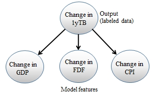
The Naive Bayes model for predicting the change in the yield of the 1-year T-bill
The correlation (or cause-effect relationship) is derived from the historical data. The methodology consists of counting the number of times each feature either increases (UP) or decreases (DOWN) and recording the corresponding expected outcome, as illustrated in the following table:
|
ID |
GDP |
FDF |
CPI |
1y-TB |
|---|---|---|---|---|
|
1 |
UP |
DOWN |
UP |
UP |
|
2 |
UP |
UP |
UP |
UP |
|
3 |
DOWN |
UP |
DOWN |
DOWN |
|
4 |
UP |
DOWN |
DOWN |
DOWN |
|
… | ||||
|
256 |
DOWN |
DOWN |
UP |
DOWN |
First, let's tabulate the number of occurrences of each change (UP and DOWN) for the three features and the output value (the direction of the change in the yield of the 1-year Treasury bill):
|
Number |
GDP |
FDF |
CPI |
1yTB |
|---|---|---|---|---|
|
UP |
169 |
184 |
175 |
159 |
|
DOWN |
97 |
72 |
81 |
97 |
|
Total |
256 |
256 |
256 |
256 |
|
UP/Total |
0.66 |
0.72 |
0.68 |
0.625 |
Next, let's compute the number of positive directions for each of the features when the yield of the 1-year Treasury bill increases (159 occurrences):
|
Number |
GDP |
Fed Funds |
CPI |
|---|---|---|---|
|
UP |
110 |
136 |
127 |
|
DOWN |
49 |
23 |
32 |
|
Total |
159 |
159 |
159 |
|
UP/Total |
0.69 |
0.85 |
0.80 |
From the preceding table, we conclude that the yield of the 1-year Treasury bill increases when the GDP increases (69 percent of the time), the rate of the Federal funds increases (85 percent of the time), and the CPI increases (80 percent of the time).
Let's formalize the Naïve Bayes model before turning these findings into a probabilistic model.
Let's start by clarifying the terminologies used in the Bayesian model:
- Class prior probability or class prior: This is the probability of a class
- Likelihood: This is the probability to observe a value or event, given a class, also known as the probability of the predictor, given a class
- Evidence: This is the probability of observations that occur, also known as the prior probability of the predictor
- Posterior probability: This is the probability of an observation x being in a given class
No model can be simpler! The log likelihood, log p(xi|Cj), is commonly used instead of the likelihood in order to reduce the impact of the features xi that have a low likelihood.
The objective of the Naïve Bayes classification of a new observation is to compute the class that has the highest log likelihood. The mathematical notation for the Naïve Bayes model is also straightforward.
Note
The Naïve Bayes classification
M1: The posterior probability p(Cj|x) is defined as:
Here, x = {xi} (0, n-1) is a set of n features. {Cj} is a set of classes with their class prior p(Cj). x = {xi} (0, n-1) with a set of n features. p(x|Cj) is the likelihood for each feature
M2: The computation of the posterior probability p(Cj| x) is simplified by the assumption of conditional independence of features:

Here, xi are independent and the probabilities are normalized for evidence p(x) = 1.
M3: The maximum likelihood estimate (MLE) is defined as:

M4: The Naïve Bayes classification of an observation x of a class Cm is defined as:
This particular use case has a major drawback—the GDP statistics are provided quarterly, while the CPI data is made available once a month and a change in FDF rate is rather infrequent.
The ability to compute the posterior probability depends on the formulation of the likelihood using historical data. A simple solution is to count the occurrences of observations for each class and compute the frequency.
Let's consider the first example that predicts the direction of the change in the yield of the 1-year Treasury bill, given changes in the GDP, FDF, and CPI.
The results are expressed with simple probabilistic formulas and a directed graphical model:
P(GDP=UP|1yTB=UP) = 110/159
P(1yTB=UP) = num occurrences (1yTB=UP)/total num of occurrences=159/256
p(1yTB=UP|GDP=UP,FDF=UP,CPI=UP) = p(GDP=UP|1yTB=UP) x
                                  p(FDF=UP|1yTB=UP) x
                                  p(CPI=UP|1yTB=UP) x
                                  p(1yTB=UP) = 0.69 x 0.85 x 0.80 x 0.625
The Bayesian network for the prediction of the change of the yield of the 1-year Treasury bill
This problem is not a good candidate for a Bayesian classification for the following two reasons:
- The training set is not large enough to compute accurate prior probabilities and generate a stable model. Decades of quarterly GDP data is needed to train and validate the model.
- The features have different rates of change, which predominately favor the features with the highest frequency; in this case, the CPI.
Let's select another use case for which a large historical dataset is available and can be automatically labeled.
The predictive model is the second use case that consists of predicting the direction of the change of the closing price of a stock, prt+1 = {UP, DOWN}, at trading day t + 1, given the history of its direction of the price, volume, and volatility for the previous t days, pri for i = 0 to i = t. The volume and volatility features have already been used in the Writing a simple workflow section in Chapter 1, Getting Started.
Therefore, the three features under consideration are as follows:
- The closing price prt of the last trading session, t, is above or below the average closing price over the n previous trading days, [t-n, t].
- The volume of the last trading day vlt is above or below the average volume of the n previous trading days
- The volatility on the last trading day vtt is above or below the average volatility of the previous n trading days
The directed graphic model can be expressed using one output variable (the price at session t + 1 is greater than the price at session t) and three features: the price condition (1), volume condition (2), and volatility condition (3).

The Bayesian model for predicting the future direction of the stock price
This model works under the assumption that there is at least one observation or ideally few observations for each feature and expected value.
It is possible that the training set does not contain any data actually observed for a feature for a specific label or class. In this case, the mean is 0/N = 0, and therefore, the likelihood is null, making classification unfeasible. The case for which there are only few observations for a feature in a given class is also an issue, as it skews the likelihood.
There are a couple of correcting or smoothing formulas for unobserved features or features with a low number of occurrences that address this issue, such as the Laplace and Lidstone smoothing formulas.
The two formulas are commonly used in natural language processing applications, for which the occurrence of a specific word or tag is a feature [5:7].
I think it is time to write some Scala code and toy around with Naïve Bayes. Let's start with an overview of the software components.
Our implementation of the Naïve Bayes classifier uses the following components:
- A generic model,
NaiveBayesModel, of theModeltype that is initialized through training during the instantiation of the class. - A model for the
BinNaiveBayesModelbinomial classification, which subclassesNaiveBayesModel. The model consists of a pair of positive and negativeLikelihoodclass instances. - A model for the
MultiNaiveBayesModelmultinomial classification. - The
NaiveBayesclassifier class has four parameters: a smoothing function, such as Laplace and a set of observations of theXVSeriestype, a set of labels of theDblVectortype, a log density function of theLogDensitytype, and the number of classes.
The principle of software architecture applied to the implementation of classifiers is described in the Design template for immutable classifiers section in the Appendix A, Basic Concepts.
The key software components of the Naïve Bayes classifier are described in the following UML class diagram:

The UML class diagram for the Naive Bayes classifier
The UML diagram omits the helper traits or classes such as Monitor or Apache Commons Math components.
The objective of the training phase is to build a model consisting of the likelihood for each feature and the class prior. The likelihood for a feature is identified as follows:
- The number of occurrences k of this feature for N > k observations in the case of binary features or counters
- The mean value for all the observations for this feature in the case of numeric or continuous features
It is assumed, for the sake of this test case, that the features, that is, technical analysis indicators, such as price, volume, and volatility are conditionally independent. This assumption is not actually correct.
Let's write the code to train the binomial and multinomial Naïve Bayes.
The first step is to define the class likelihood for each feature using historical data. The Likelihood class has the following attributes (line 1):
- The label for the
labelobservation - An array of tuple Laplace or Lidstone smoothed mean and standard deviation,
muSigma - The prior probability of a
priorclass
As with any code snippet presented in this book, the validation of class parameters and method arguments are omitted in order to keep the code readable:
class Likelihood[T <: AnyVal](
     val label: Int,
     val muSigma: Vector[DblPair],
     val prior: Double)(implicit f: T => Double)  {  //1

  def score(obs: Array[T], logDensity: LogDensity): Double = //2
    (obs, muSigma).zipped
     .map{ case(x, (mu,sig)) => (x, mu, sig)}
     ./:(0.0)((prob, entry) => {
         val x = entry._1
         val mean = entry._2
         val stdDev = entry._3
         val logLikelihood = logDensity(mean, stdDev, x) //3
         val adjLogLikelihood = if(logLikelihood <MINLOGARG)
                     MINLOGVALUE else logLikelihood)
         prob + Math.log(adjLogLikelihood) //4
   }) + Math.log(prior)
}
The parameterized Likelihood class has the following two purposes:
- Define the statistics regarding a class Ck: its label, its mean and standard deviation, and the prior probability p(Ck).
- Compute the score of a new observation for its runtime classification (line
2). The computation of the log of the likelihood uses alogDensitymethod of theLogDensitytype (line3). As seen in the next section, the log density can be either a Gaussian or a Bernoulli distribution. Thescoremethod uses Scala'szippedmethod to merge the observation values with the labeled values and implements the M3 formula (line4).
The Gaussian mixture is particularly suited for modeling datasets, for which the features have large sets of discrete values or are continuous variables. The conditional probabilities for the feature x is described by the normal probability density function [5:9].

The log of the Gauss, logGauss, and the log of the Normal distribution, logNormal, are defined in the stats class, which was introduced in the Profiling data section in Chapter 2, Hello World!:
def logGauss(mean: Double, stdDev: Double, x: Double): Double ={
  val y = (x - mean)/stdDev
  -LOG_2PI - Math.log(stdDev) - 0.5*y*y
}
val logNormal = logGauss(0.0, 1.0, _: Double)
The logNormal computation is implemented as a partial applied function.
The functions of the LogDensity type compute the probability density for each feature (line 5):
type LogDensity = (Double*) => DoubleThe next step is to define the BinNaiveBayesModel model for a two-class classification scheme. The two-class model consists of two Likelihood instances: positives for the label UP (value 1) and negatives for the label DOWN (value 0).
In order to make the model generic, we created a NaiveBayesModel trait that can be extended as needed to support both the binomial and multinomial Naïve Bayes models, as follows:
trait NaiveBayesModel[T]  {
  def classify(x: Array[T], logDensity: LogDensity): Int //5
}
The classify method uses the trained model to classify a multivariate observation x of the Array[T] type given a logDensity probability density function (line 5). The method returns the class the observation belongs to.
Let's start with the definition of the BinNaiveBayesModel class that implements the binomial Naïve Bayes:
class BinNaiveBayesModel[T <: AnyVal](
    pos: Likelihood[T],
    neg: Likelihood[T])(implicit f: T => Double)
  extends NaiveBayesModel[T] { //6

  override def classify(x: Array[T], logDensity: logDensity): Int = //7
   if(pos.score(x,density) > neg.score(x,density)) 1 else 0
  ...
}
The constructor for the BinNaiveBayesModel class takes two arguments:
pos: Class likelihood for observations with a positive outcomeneg: Class likelihood for observations with a negative outcome (line6)
The classify method is called by the |> operator in the Naïve Bayes classifier. It returns 1 if the observation x matches the Likelihood class that contains the positive cases, and 0 otherwise (line 7).
Note
Model validation
The parameters of the Naïve Bayes model (likelihood) are computed through training and the model value is instantiated regardless of whether the model is actually validated in this example. A commercial application would require the model to be validated using a methodology such as the K-fold validation and F1 measure, as described in the Design template for immutable classifiers section in the Appendix A, Basic Concepts.
The multinomial Naïve Bayes model defined by the MultiNaiveBayesModel class is very similar to the BinNaiveBayesModel:
class MultiNaiveBayesModel[T <: AnyVal(   //8
   likelihoodSet: Seq[Likelihood[T]])(implicit f: T => Double)
  extends NaiveBayesModel[T]{

  override def classify(x: Array[T], logDensity: LogDensity): Int = {
    val <<< = (p1: Likelihood[T], p2: Likelihood[T]) =>
              p1.score(x, density) > p1.score(x, density) //9
    likelihoodSet.sortWith(<<<).head.label  //10
  }
  ...
}
The multinomial Naïve Bayes model differs from its binomial counterpart as follows:
- Its constructor requires a sequence of class likelihood
likelihoodSet(line8). - The
classifyruntime classification method sorts the class likelihoods by their score (posterior probability) using the<<<function (line9). The method returns the ID of the class with the highest log likelihood (line10).
The Naïve Bayes algorithm is implemented as a data transformation using a model implicitly extracted from a training set of the ITransform type, as described in the Monadic data transformation section in Chapter 2, Hello World!
The attributes of the multinomial Naïve Bayes are as follows:
- The smoothing formula (Laplace, Lidstone, and so on),
smoothing - The set of multivariable observations defined as
xt - The expected values (or labels) associated with the set of observations,
expected - The log of the probability density function,
logDensity - The number of classes—two for the binomial Naïve Bayes with the
BinNaiveBayesModeltype or more for the multinomial Naïve Bayes with theMultiNaiveBayesModeltype (line11)
The code will be as follows:
class NaiveBayes[T <: AnyVal](
    smoothing: Double,
    xt: XVSeries[T],
    expected: Vector[Int],
    logDensity: LogDensity,
    classes: Int)(implicit f: T => Double)
  extends ITransform[Array[T]](xt)
    with Supervised[T, Array[T]] with Monitor[Double] { //11
  type V = Int  //12
  val model: Option[NaiveBayesModel[T]]  //13
  def train(expected: Int): Likelihood[T]
  …
}
The Monitor trait defines miscellaneous logging and display functions.
Data transformation of the ITransform type requires the output type V to be specified (line 12). The output of the Naïve Bayes is the index of the class an observation belongs to. The model type of the model can be either BinNaiveBayesModel for two classes or MultiNaiveBayesModel for a multinomial model (line 13):
val model: Option[NaiveBayesModel[T]] = Try {
  if(classes == 2)
    BinNaiveBayesModel[T](train(1), train(0))
  else
    MultiNaiveBayesModel[T](List.tabulate(classes)( train(_)))
} match {
  case Success(_model) => Some(_model)
  case Failure(e) => /* … */
}
Note
Training and class instantiation
There are several benefits of allowing the instantiation of the Naïve Bayes mode only once when it is trained. It prevents the client code from invoking the algorithm on an untrained or partially trained model, and it reduces the number of states of the model (untrained, partially trained, trained, validated, and so on). It is an elegant way to hide the details of the training of the model from the user.
The train method is applied to each class. It takes the index or label of the class and generates its log likelihood data (line 14):
def train(index: Int): Likelihood[T] = {   //14
  val xv: XVSeries[Double] = xt
  val values = xv.zip(expected) //15
               .filter( _._2 == index).map(_._1) //16
  if( values.isEmpty )
     throw new IllegalStateException( /* ... */)

  val dim = dimension(xt)
  val meanStd = statistics(values).map(stat =>
         (stat.lidstoneMean(smoothing, dim), stat.stdDev)) //17
  Likelihood(index, meanStd, values.size.toDouble/xv.size) //18
}
The training set is generated by zipping the xt vector of observations with expected classes, expected (line 15). The method filters out the observation for which the label does not correspond to this class (line 16). The meanStd pair (mean and standard deviation) is computed using the Lidstone smoothing factor (line 17). Finally, the training method returns the class likelihood corresponding to the index label (line 18).
The NaiveBayes class also defines the |> runtime classification method and the F1 validation methods. Both methods are described in the next section.
Note
Handling missing data
Naïve Bayes has a no-nonsense approach to handling missing data. You just ignore the attribute in the observations for which the value is missing. In this case, the prior for this particular attribute for these observations is not computed. This workaround is obviously made possible because of the conditional independence between features.
The apply constructor for NaiveBayes returns the NaiveBayes type:
object NaiveBayes {
  def apply[T <: AnyVal](
        smoothing: Double,
        xt: XVSeries[T],
        expected: Vector[Int],
        logDensity: LogDensity,
        classes: Int) (implicit f: T => Double): NaiveBayes[T] =
    new NaiveBayes[T](smoothing, xt, y, logDensity, classes)
   …
}The likelihood and class prior that have been computed through training is used for validating the model and classifying new observations.
The score represents the log of likelihood estimate (or the posterior probability), which is computed as the summation of the log of the Gaussian distribution using the mean and standard deviation extracted from the training phase and the log of the class likelihood.
The Naïve Bayes classification using the Gaussian distribution is illustrated using the two C1 and C2 classes and a model with two features (x and y):

An illustration of the Gaussian Naive Bayes using 2-dimensional model
The |> method returns the partial function that implements the runtime classification of a new x observation using one of the two Naïve Bayes models. The model and the logDensity functions are used to assign the x observation to the appropriate class (line 19):
override def |> : PartialFunction[Array[T], Try[V]] = {
  case x: Array[T] if(x.length >0 && model != None) =>
    Try( model.map(_.classify(x, logDensity)).get)  //19
}
Finally, the Naïve Bayes classifier is implemented by the NaiveBayes class. It implements the training and runtime classification using the Naïve Bayes formula. In order to force the developer to define a validation for any new supervised learning technique, the class inherits from the Supervised trait that declares the validate validation method:
trait Supervised[T, V] {
  self: ITransform[V] =>  //20
    def validate(xt: XVSeries[T],
      expected: Vector[V]): Try[Double]  //21
}
The validation of a model applies only to a data transformation of the ITransform type (line 20).
The validate method takes the following arguments (line 21):
- An
xttime series of multidimensional observations - An
expectedvector of expected class values
By default, the validate method returns the F1 score for the model, as described in the Assessing a model section in Chapter 2, Hello World!
Let's implement the key functionality of the Supervised trait for the Naïve Bayes classifier:
override def validate(
    xt: XVSeries[T],
    expected: Vector[V]): Try[Double] =  Try {   //22
  val predict = model.get.classify(_:Array[Int],logDensity) //23
  MultiFValidation(expected, xt, classes)(predict).score  //24
}
The predictive predict partially applied function is created by assigning a predicted class to a new x observation (line 23), and then the prediction, the index of classes, is loaded into the MultiFValidation class to compute the F1 score (line 24).
The most critical element in the training of a supervised learning algorithm is the creation of labeled data. Fortunately, in this case, the labels (or expected classes) can be automatically generated. The objective is to predict the direction of the price of a stock for the next trading day, taking into account the moving average price, volume, and volatility over the last n days.
The extraction of features follows these six steps:
- Extract historical trading data of each feature (that is, price, volume, and volatility).
- Compute the simple moving average of each feature.
- Compute the difference between the value and moving average of each feature.
- Normalize the difference by assigning 1 for positive values and 0 for negative values.
- Generate a time series of the difference between the closing price of the stock and the closing price of the previous trading session.
- Normalize the difference by assigning 1 for positive values and 0 for negative values.
The following diagram illustrates the feature extractions for steps 1 to 4:

Binary quantization of the difference value—moving average
The first step is to extract the average price, volume, and volatility (that is, 1 – low/high) for each stock during the period of Jan 1, 2000 and Dec 31, 2014 with daily and weekly closing prices. Let's use the simple moving average to compute these averages for the [t-n, t]window.
The extractor variable defines the list of features to extract from the financial data source, as described in the Data extraction and Data sources section in the Appendix A, Basic Concepts:
val extractor = toDouble(CLOSE)  // stock closing price
               :: ratio(HIGH, LOW) //volatility(HIGH-LOW)/HIGH
               :: toDouble(VOLUME)  // daily stock trading volume
               :: List[Array[String] =>Double]()
The naming convention for the trading data and metrics is described in the Trading data section under Technical analysis in the Appendix A, Basic Concepts.
The training and validation of the binomial Naïve Bayes is implemented using a monadic composition:
val trainRatio = 0.8  //25
val period = 4
val symbol ="IBM"
val path = "resources/chap5"
val pfnMv = SimpleMovingAverage[Double](period, false) |> //26
val pfnSrc = DataSource(symbol, path, true, 1) |>  //27

for {
  obs <- pfnSrc(extractor)  //28
  (x, delta) <- computeDeltas(obs) //29
  expected <- Try{difference(x.head.toVector, diffInt)}//30
  features <- Try { transpose(delta) } //31
  labeled <- //32
     OneFoldXValidation[Int](features, expected, trainRatio)
  nb <- NaiveBayes[Int](1.0, labeled.trainingSet) //33
  f1Score <- nb.validate(labeled.validationSet) //34
}
yield {
  val labels = Array[String](
    "price/ave price", "volatility/ave. volatility",
    "volume/ave. volume"
  )
  show(s"
Model: ${nb.toString(labels)}")
}
The first step is to distribute the observations between the training set and validation set. The trainRatio value (line 25) defines the ratio of the original observation set to be included in the training set. The simple moving average values are generated by the pfnMv partial function (line 26). The extracting pfnSrc partial function (line 27) is used to generate the three trading time series, price, volatility, and volume (line 28).
The next step consists of applying the pfnMv simple moving average to the obs multidimensional time series (line 29) using the computeRatios method:
type LabeledPairs = (XVSeries[Double], Vector[Array[Int]])

def computeDeltas(obs: XVSeries[Double]): Try[LabeledPairs] =
Try{
  val sm = obs.map(_.toVector).map( pfnMv(_).get.toArray) //35
  val x = obs.map(_.drop(period-1) )
  (x, x.zip(sm).map{ case(x,y) => x.zip(y).map(delta(_)) })//36
}
The computeDeltas method computes the time series of the sm observations smoothed with a simple moving average (line 35). The method generates a time series of 0 and 1 for each of the three features in the xs observation set and sm smoothed dataset (line 36).
Next, the call to the difference differential computation generates the labels (0 and 1) representing the change in the direction of the price of a security between two consecutive trading sessions: 0 if the price is decreased and 1 if the price is increased (line 30) (refer to the The differential operator section under Time series in Scala in Chapter 3, Data Preprocessing).
The features for the training of the Naïve Bayes model are extracted from these ratios by transposing the ratios-time series matrix in the transpose method of the XTSeries singleton (line 31).
Next, the training set and validation set are extracted from the features set using the OneFoldXValidation class, which was introduced in the One-fold cross validation section under Cross-validation in Chapter 2, Hello World! (line 32).
Note
Selecting the training data
In our example, the training set is simplistically the first trainRatio multiplied by the size of dataset observations. Practical applications use a K-fold cross-validation technique to validate models, as described in the K-fold cross validation section under Assessing a model in Chapter 2, Hello World!. A simpler alternative is to create the training set by picking observations randomly and using the remaining data for validation.
The last two stages in the workflow consists of training the Naïve Bayes model by instantiating the NaiveBayes class (line 33) and computing the F1 score for different values of the smoothing coefficient of the simple moving average applied to the stock price, volatility, and volume (line 34).
Note
The implicit conversion
The NaiveBayes class operates on elements of the Int and Double types, and therefore, assumes that there is conversion between Int and Double (view bounded). The Scala compiler may generate a warning because the conversion from Int to Double has not been defined. Although Scala relies on its own conversion functions, I would recommend that you explicitly define and control your conversion function:
implicit def intToDouble(n: Int): Double = n.toDouble
The next chart plots the value of the F1 measure of the predictor of the direction of the IBM stock using price, volume, and volatility over the previous n trading days, with n varying from 1 to 12 trading days:

A graph of the F1-measure for the validation of the Naive Bayes model
The preceding chart illustrates the impact of the value of the averaging period (number of trading days) on the quality of the multinomial Naïve Bayes prediction, using the value of the stock price, volatility, and volume relative to their average over the averaging period.
From this experiment, we conclude the following:
- The prediction of the stock movement using the average price, volume, and volatility is not very good. The F1 score for the models using weekly (with respect to daily) closing prices varies between 0.68 and 0.74 (with respect to 0.56 and 0.66).
- The prediction using weekly closing prices is more accurate than the prediction using the daily closing prices. In this particular example, the distribution of the weekly closing prices is more reflective of an intermediate term trend than the distribution of daily prices.
- The prediction is somewhat independent of the period used to average the features.