
This chapter presents a dynamic and aggregate QoS mapping control in which streaming video senders, video receivers, and a special boundary node (which we refer to as CM gateway, or video gateway (VG), specifically for streaming videos, located at the border of a DS domain) interact with one another to control all incoming video streaming QoS to the VG to provide stable DiffServ under time-varying network conditions in a totally cost-effective manner. The video application at the source grades the chunks (i.e., packets) of its content by certain indices in accordance with their importance in end-to-end QoS (e.g., in terms of loss probability and delay). Since these indices reflect the desired service preference of one portion with respect to other portions, we denote it as the RPI, which is further divided into the RLI and RDI, respectively (see Chapter 3). The QoS mapping control takes place at the VG in the form of assigning each packet an appropriate DS level while considering all incoming aggregate flows. The VG, as a special case of a media gateway, is responsible for this QoS mapping at the ingress of a DS domain and for managing traffic in accordance with the TCA specified in the SLA with the DS domain.
The rest of this chapter is organized as follows. In Section 5.2, we briefly describe the proposed dynamic QoS mapping control composed of feedforword and feedback QoS mapping control in the VG with three different granularity. Video categorization with source importance was examined in Chapter 3 and is used here for QoS mapping control between applications and network DS levels. Section 5.3 presents dynamic QoS mapping control through traffic conditioning and feedback reaction at the VG. Section 5.4 provides the analysis of proposed aggregated traffic marker as a key traffic-conditioning function. Various sets of performance evaluation based on computer simulation are presented in Section 5.5. Concluding remarks are given in Section 5.6.
The architecture that we propose is illustrated in Figure 5.1. Sources (end-systems storing video content) within the customer network (customer of the DS domain) send video to the video clients. The traffic leaves the customer network through the VG. The customer network subscribes to DS services, and traffic is delivered to the clients through the DS domain. The customer network has SLAs [17] with the DS domain. A video source has, for each video packet, an associated RPI computed on the basis of the packet’s importance for the quality of the entire video stream. An RPI is a real number, and its meaning was discussed in Section 3.3. The source divides the video packets into categories, each of which is represented by an integer k. The categories can be simply interpreted as the discretization of RPIs. The source then furnishes each packet with this categorization information (value of k) for the VG when it sends the packet stream to the VG. The VG forwards the packet streams to their respective clients through the DS domain. Thus, the video streams from the sources merge in the VG.

The main functions of the VG are to assign to each packet a DSCP and to dynamically schedule each packet’s transmission into the DS domain on the basis of the packet’s categories (k number) and traffic conditions. This codepoint assignment can be viewed as a mapping from category (k) to DS behavior aggregate (BA), which we represent by another integer variable, q. (We will use the phrases “behavior aggregate” and “DS level” interchangeably.)
The VG must observe the TCA in the SLA with the DS domain, so the goal of the VG is to achieve the best video quality at the client side within the constraints of the TCA. Unlike the sources, the VG can observe the traffic behavior of all the video streams going through it. Thus, the VG can assign a DS level to a packet from the perspective of corporate video stream quality.
To share the DS services fairly among the sources and protect resources from a selfish source, the VG exercises traffic shaping on a per-flow basis through the token buckets (TBs) assigned for individual flows (sessions), as seen in Figure 5.1. (There is an agreement between the source and the VG regarding the allowable traffic behavior for each session.) Packets violating this agreement (enforced by the TB) are assigned the lowest DS level (best-effort grade). For packets conforming to the TB, the VG performs the k-to-q mapping (DS marking) for each flow individually on the basis of quality optimization, which was discussed in detail in Section 3.4. Then, the flows with packets are marked with DSCPs merge at the traffic-conditioning module, which adjusts the codepoints on the basis of the dynamically varying traffic load to satisfy the TCA. The function of the traffic management module will be discussed in more detail in Section 5.3.1.
Each CM application will demand its loss rate/delay preference by marking its DS field based on the RPI, which comprises both the RLI and RDI. That is, CM packets are categorized by the RLI/RDI, and the DS byte (i.e., DiffServ codepoint: DSCP) is marked accordingly based on the discussion in Section 3.3. With this, we are supporting packet-based differentiation granularity. Each packet from a CM session undergoes the bandwidth restriction enforced by the TB, especially for peak rate, to prevent a user from abusing shared bandwidth. Non-conforming traffic packets of the per-user TB are marked with the best-effort service label (i.e., the lowest service class). Categorized CM flows are then aggregated at the VG, which is responsible for aggregate QoS mapping at the ingress of a DiffServ domain and for managing traffic in accordance with the TCA specified in the SLA with the DiffServ domain. In our approach, we have adopted a bundle of TB-based markers (TMs) we call a two-rate, three-color marker (trTCM) [116], described in detail in Section 5.3.1, to handle traffic conditioning for aggregated flows while trying to provide dynamic and effective QoS mapping.
In this environment, we are focusing on the dynamic and aggregate QoS mapping control at the VG for CM applications. As shown in Figure 5.1, two kinds of mechanisms are used: feedforward and feedback. With feedforward QoS control, which is the default mode of operation covering all three levels of granularity, we treat effective QoS mapping between aggregate, categorized CM packets and network DS levels under the SLA. A more detailed algorithm for feedforward QoS mapping will be discussed in Section 5.3.1. Complementary feedback QoS mapping control assumes that there is feedback support from end-systems covering session-based granularity only. By adjusting the mapping categorization of RPI into the network level (i.e., k → q) based on the receiver’s feedback report, the quality of streaming video can be better managed. This process provides dynamic QoS mapping adjustment between end-systems that are connected as fine-grain. Feedback in terms of the end-to-end quality as well as the associated delay/loss status is relayed back to the corresponding sender. Note that the VG is also capable of handling this feedback. However, leveraging what the intelligent end-system with the RPI categorization is already doing seems a natural choice. A more detailed algorithm is described in Section 5.3.2.
Based on the per-flow QoS mapping guidance in Section 3.4.2, we move on to the dynamic case (i.e., time-varying network service quality) for aggregate flows. In a real situation, the proposed QoS mapping should incorporate additional issues that cannot be assumed. First, in general, because the whole distribution of the RPI is not available at starting time for QoS mapping, the VG should try to do the best mapping of a flow with only the known, observed RPIs or categorized RPIs. Next, we cannot assume that the DS domain can provision the ideal proportional differentiated service over all time intervals. Another implication that a real situation presents is that we need to limit the resource allocation based on the TCA specified in the SLA with the DiffServ domain. To address all of these limitations, a dynamic QoS mapping mechanism is necessary beyond the per-flow QoS mapping guidelines discussed in Section 3.4. As shown in Figure 5.1, dynamic QoS mapping is done for aggregated flows at the VG in feedforward/feedback mode.
The overall feedforward QoS mapping control algorithm at the VG is summarized in Figure 5.2.
A video packet is categorized into a k category by the RLI/RDI at the video sender without knowledge of other competing flows. An assigned RDI may limit the mapping range of q, as discussed earlier. Then, the key issue becomes how to perform practical and effective QoS mapping based on Eq. (3.12). First, from Figures 3.12 and 3.13, we can obtain a practical mapping guidance for k → q mapping by considering session/packet-based granularity. Also, within the customer network, traffic conditioning per end-user is handled by the VG via the assignment of a TB with different parameters (e.g., the token rate, bucket size, etc.). The total sending rate is restricted by the pre-assigned total bandwidth usage per end-user. In addition, the total cost constraint may be applied, which altogether covers a per-user QoS mapping control in session-/packet-based granularity. Note that the proposed dynamic QoS mapping scheme helps end-users minimize quality distortion under the total price paid.
Dynamic QoS mapping for class-based granularity is performed by re-marking through the traffic-conditioning function. By degrading the k → q mapping level when a flow or a class traffic volume exceeds the allowed bandwidth, we can regulate the traffic while trying to meet per-flow efficiency as detailed below.
An access network operator can contract with an ISP for a TCA in the SLA. Because an end-user is blind to aggregate flows entering the DS domain (including flows from other end-users), we force the VG to perform traffic conditioning for DS levels on aggregate flows. The procedure for re-marking in accordance with the TCA should be designed on the basis of the services provided by the DS domain and SLA. In this chapter, we target our design and simulation for AF services. For the SLA, we take the example of parameters such as the committed burst size (CBS), committed information rate (CIR), peak burst size (PBS), peak information rate (PIR), etc. We assume that the TCA between the access network and DS domain is the conditioning described by the trTCM. We also assume that a separate trTCM is operating for each of the three AF classes.
Each trTCM is composed of two TBs, C and P for CBS and PBS, respectively, to meter incoming packets and mark them with one of three colors: green, yellow, or red. For this chapter, we consider an example case in which the access network subscribes to three AF classes, and that each AF class further differentiates the packets into three kinds of drop precedence. The access network can also use best-effort service. We denote the resulting DS levels (BAs) by BE and AFxy. BE denotes the best-effort level and AFxy denotes the BA of the AF class x ∊ {1,2,3} and drop precedence y ∊ {1,2,3}. We assume that our QoS parameter q is associated with the following DS levels: BE, AF33, AF32, AF31, AF23, AF22, AF21, AF13, AF12, and AF11, which are equivalent to the numbers q = 0 - 9 in this work. (We are assuming that the lowest drop precedence of AF Class 1 provides better packet drop probability than the highest drop precedence of AF Class 2, etc.) For adopting trTCM, we use the following color coding:
Green—. Corresponds to DS level AFx1
Yellow—. Corresponds to DS level AFx2
Red—. Corresponds to DS level AFx3
We use the color-aware mode of trTCM for re-marking. Because k → q mapping is done prior to the aggregate traffic conditioning (Figure 5.3), and because the value of q specifies the color and AF class, the traffic input to the trTCM can be considered already color-coded.
In the color-aware mode, packets arrive with some pre-assigned color. The initial assignment is respected, and the drop precedence can only be increased. TBs P and C are initialized to CBS and PBS in the beginning. Token bytes BC (for the C token bucket) and BP (for the P TB) are incremented by CIR and PIR up to their upper bounds, CBS and PBS, respectively.
If a packet of size B has been colored red, it will remain red. A yellow packet is re-marked as red if there is no token available in both the C and P buckets. Otherwise, it is allowed to remain yellow, and Bp becomes BP – B if there is, for example, a token in the P bucket. Finally, a green packet becomes yellow with BP ← BP – B only if a token is available in the P bucket. It becomes red if there is no token available in either bucket. Otherwise, a green packet remains green with BC ← BC – B and BP ← BP – B.
To improve the end-to-end quality of video delivery beyond just satisfying the TCA, we modify the individual trTCMs into “interconnected trTCM.” To coordinate the interconnected function between trTCMs, the aggregated ingress rate into each class is measured. When the aggregated rate reaches the maximum assigned rate Cj for each class queue with a typical WFQ scheduler, as shown in Figure 5.3, we hand over the incoming packet randomly. The aggregated ingress rate is calculated by using exponentially weighted moving averaging to smooth the estimation of fluctuation noise. To avoid possible sensitivity due to packet length distribution, dynamic weighting as a function of inter-packet arrival time is utilized. Thus, the average rate is measured via
where current_rate can be calculated as (arrived packet size)/(inter-packet time), with T as a constant. Refer to [29] for more details regarding the choice of T.
In interconnected trTCM, if the aggregated rate for the queue of class j is greater than Cj, the packets coming into this queue are re-directed by trTCM to a lower class queue with the probability of (avg_rate – Cj)/avg_rate, and so on. When a packet is re-directed to a lower AF class, the color is set to green in that lower class.
With the above schemes in place, we believe that the VG can reduce the probability of end-to-end service inversion (i.e., a lower class flow happens to receive better service than a higher class one), which will be suggested in the simulation result to be presented in Section 5.5. In fact, we plan to investigate the merits of including interconnected trTCM as part of a TCA. If all access points to the DS domain exercise trTCM, the probability of service inversion within the DS domain may be greatly reduced.
Feedback control is performed by the VG with the support of end-systems to adjust the QoS mapping level of the RLI to category k and the RDI level for delay quality on feedback from the video receiver. The receiver sends a report of delay/packet loss to the sender whenever necessary and can ask for a mapping adjustment when the received quality is not satisfactory. This feedback control enables the fine-tuning of rather coarse feedforward QoS mapping. The video receiver may even ask for a decrease in the QoS mapping level if it feels the current received quality is over-provisioned and it wants to reduce costs. This feedback mechanism enables the whole QoS control to be more efficiently adjusted and to remain stable by sustaining end-to-end quality within an acceptable range. The algorithm for the feedback QoS control is summarized in Figure 5.4.

If the aggregated rate for the queue of class j is greater than Cj, the packets coming into this queue are re-directed by trTCM to lower the class queue with the downgrading probability DPd, and so on. The excessive portion over Cj can be divided into two parts as a more general case: (1) parts downgraded to a lower class with a probability ![]() , and (2) parts remaining in the same class as red-marked packets that are susceptible to being dropped with a corresponding probability
, and (2) parts remaining in the same class as red-marked packets that are susceptible to being dropped with a corresponding probability ![]() when the incoming rate in a class queue j exceeds the assigned rate Cj:
when the incoming rate in a class queue j exceeds the assigned rate Cj:
We can leave the partition ratio of the excessive portion to the ISP as a controllable knob of overall packet loss rates of BAs.
In short, the proposed aggregate traffic marker checks traffic packets with orders ranging from higher to lower priority BAs and performs the re-marking of packets randomly with the probabilities ![]() and
and ![]() in accordance with the aggregate rate. It is a combined approach of TB- and rate-based. The proposed aggregate traffic marker in boundary node (BN) enables the DS domain to provide more reliable differentiated services among BAs or DiffServ classes.
in accordance with the aggregate rate. It is a combined approach of TB- and rate-based. The proposed aggregate traffic marker in boundary node (BN) enables the DS domain to provide more reliable differentiated services among BAs or DiffServ classes.
The focus of this analysis is to show how the proposed algorithm works properly in a worst-case scenario of overload and unbalanced conditions. The other well-provisioned cases and heavily loaded lower class queues do not cause service conversion in terms of QoS parameters such as packet loss, throughput, and delay/jitter. Throughput can be estimated directly from the loss rate for user datagram protocol (UDP)- based traffic as a one-way media stream, and there are several throughput models [117] for TCP-based traffic, including a source rate-adaptive one. We will show that delay and jitter in a MQ system with a WFQ scheduler are bounded and calculated if queue per traffic is characterized by parameters such as {average rate, burst depth} [55].
In this section, we mainly perform loss analysis. And we consider only a worst-case scenario in which all aggregate rates of AFj1, ![]() are greater than CIRj, that is,
are greater than CIRj, that is, ![]() for j ∊ {1, 2,...K} if K AF class queues exist. Also, the sum of the aggregate flows of AFj1 and AFj2,
for j ∊ {1, 2,...K} if K AF class queues exist. Also, the sum of the aggregate flows of AFj1 and AFj2, ![]() is greater than PIRj, and the total sum of the aggregate rates of AFj,
is greater than PIRj, and the total sum of the aggregate rates of AFj, ![]() is greater than Cj.
is greater than Cj.
Generally, we can define the probability of marking packets as green after they pass through the traffic marker as Pg, which is a function of variable sg:

The probability of handing over parts of green packets to tentatively yellow-marked packets, P(g,y), is ![]() . Next, if the aggregate rate of both green and yellow pre-marked packets, sg + sy, is greater than PIR, we can define the probability of marking packets as yellow after they have passed through marker Py as
. Next, if the aggregate rate of both green and yellow pre-marked packets, sg + sy, is greater than PIR, we can define the probability of marking packets as yellow after they have passed through marker Py as ![]() . Similarly, the probability of handing over parts of yellow packets to tentatively red packets is P(y,r) = 1 – Py:
. Similarly, the probability of handing over parts of yellow packets to tentatively red packets is P(y,r) = 1 – Py:

Then, the probability of marking green packets as tentatively red packets, P(g,r), is P(g,y) · P(y,r) is expressed as follows:
The probability of red-marked packets, Pr, including the handed-over portions amounting to P(g,r) and P(y,r) from sg and sy, respectively, which remain red after the processing of the marker, is ![]() , where Rt = sg + sy + sr.
, where Rt = sg + sy + sr.
Next, the loss probabilities of each BA, named as red, yellow, or green here, will be calculated in Sections 5.4.1 and 5.4.2 for the cases of existing “isolated trTCM” and proposed “interconnected trTCM.”
This is the case in which each AF class has one corresponding trTCM and there is no portion obtained by re-marking an AF class into a lower AF class because of an isolated trTCM per AF class, even though the total sum of the aggregate rates of AFj, ![]() is greater than Cj.
is greater than Cj.
We will assume that multiple RED, used as queue management for outflowing packets after they have passed through the aggregate traffic marker, provides perfect service differentiation, including dropping red-marked packets before yellow packets and yellow packets before green packets. The drop probability among red-marked packets, ![]() , is defined as
, is defined as  , where
 ![]() . This means that the portion of each AF class that exceeds the assigned bandwidth Cj is exposed to being dropped, not downgraded, in the isolated trTCM case:
. This means that the portion of each AF class that exceeds the assigned bandwidth Cj is exposed to being dropped, not downgraded, in the isolated trTCM case:

The loss probability of packets pre-marked as green before entering trTCM, ![]() , is
, is ![]() ·
· ![]() , and the loss probability of originally yellow-marked packets,
, and the loss probability of originally yellow-marked packets, ![]() , is
, is ![]() ·
· ![]() .
.
In summary, we have derived the loss probabilities of pre-marked packets coming into isolated trTCM per each AFj class as green, yellow, and red to be ![]() ,
, ![]() , and
, and ![]() , respectively.
, respectively.
As a proposed case, we connect each trTCM per AF class and establish a serial link in accordance with the priority orders, that is, AF1 > AF2 > ... > AFk. Also, the downgrading probability ![]() is introduced, in addition to
is introduced, in addition to ![]() , which was provided in Section 5.4.1.
, which was provided in Section 5.4.1. ![]() is defined as a forced dropping probability among red packets by dropper or queue managements when the whole portion that exceeds Cj is not totally downgraded into a lower AF class. Then, some parts of the whole excessive portion are dropped with a probability of
is defined as a forced dropping probability among red packets by dropper or queue managements when the whole portion that exceeds Cj is not totally downgraded into a lower AF class. Then, some parts of the whole excessive portion are dropped with a probability of ![]() , and other parts are handed over to green packets in a lower AFj+1 class with a probability of
, and other parts are handed over to green packets in a lower AFj+1 class with a probability of ![]() .
.

We can adjust the probabilities ![]() and
and ![]() for the purpose of loss control as a control knob of the ISP. The loss probability of pre-marked green packets in the AF1 class can be expressed as follows:
for the purpose of loss control as a control knob of the ISP. The loss probability of pre-marked green packets in the AF1 class can be expressed as follows:

where DPBE is the drop probability of the BE traffic class. The last trTCM for the AFK class finally re-marks the parts of its red packets exceeding the assigned CK rate as the default BE class. Similarly, ![]() or
or ![]() can be obtained from Eq. (5.6) by substituting
can be obtained from Eq. (5.6) by substituting ![]() or
or ![]() for
for ![]() . Loss probabilities of other AF classes can be obtained in a similar fashion.
. Loss probabilities of other AF classes can be obtained in a similar fashion.
For simplicity without loss of generality, if we assume that the whole portion exceeding Cj is downgraded fully (i.e., ![]() ), then Eq. (5.5) becomes
), then Eq. (5.5) becomes ![]() .
.
Only the third term of the last equation of Eq. (5.6) remains. When we consider only ![]() , then the loss probabilities of the AF1 class are as follows:
, then the loss probabilities of the AF1 class are as follows:

The loss probabilities of the other AF classes are easily obtained from Eq. (5.7) by changing indices. Note that the amount downgraded ![]() for j ∊ {2, 3...K}, should be considered in calculating
for j ∊ {2, 3...K}, should be considered in calculating ![]() and
and ![]() of Eq. (5.2) and (5.3), instead of sg. Namely, the total summed amount of green-marked packets for a lower jth AF class is:
of Eq. (5.2) and (5.3), instead of sg. Namely, the total summed amount of green-marked packets for a lower jth AF class is:

where the index j = 1 indicates the highest priority queue that does not have a downgraded portion from the other queues.
Note that the TB sizes in TCA, CBS, and PBS can help to absorb a momentary burst up to the maximum peak rate, such as pg(t) = CBS + CIR · t and py(t) = PBS + (PIR – CIR) · t, but not a persistent burst. The TB sizes serve as low-pass filtering and have a smoothing effect on the instantaneous burst rate of each BA so that it can conform to the subscribed profile, which includes long-term average rate, CIR, and PIR. Therefore, TB sizes should also be included in the TCA. In summary, our analysis of average rate is enough to evaluate the overall performance of the proposed aggregate traffic marker.
First, we compare the performance of the two cases in Section 5.4.4. Then we draw loss probabilities ![]() ,
, ![]() , and
, and ![]() , derived in Section 5.4.4, for a three-class queue system: AF1, AF2, and BE. The ratio of the weighting factor of the WFQ scheduler is equivalent to the ratio of the common link rate because C1 = 2 · C2 for the AF1 and AF2 class queues and C2 = 2 · CBE for the AF2 and BE class queues. For each AF class queue, we set CIR = Cj/4, and PIR = 2 · CIR. The ranges of the sending rates of the BAs are sg = [CIR, C] for AFj1, sy = [PIR – CIR, C] for AFj2, and sr = Cj for PIR, respectively. For simplicity, the sending rate of red packets for each AF class, sr, is chosen as the maximum conformed rate Cj – PIR. The other aggregate sending rates of green and yellow for each AF class vary over the defined ranges.
, derived in Section 5.4.4, for a three-class queue system: AF1, AF2, and BE. The ratio of the weighting factor of the WFQ scheduler is equivalent to the ratio of the common link rate because C1 = 2 · C2 for the AF1 and AF2 class queues and C2 = 2 · CBE for the AF2 and BE class queues. For each AF class queue, we set CIR = Cj/4, and PIR = 2 · CIR. The ranges of the sending rates of the BAs are sg = [CIR, C] for AFj1, sy = [PIR – CIR, C] for AFj2, and sr = Cj for PIR, respectively. For simplicity, the sending rate of red packets for each AF class, sr, is chosen as the maximum conformed rate Cj – PIR. The other aggregate sending rates of green and yellow for each AF class vary over the defined ranges.
For a fair comparison of the two cases, we choose a drop probability LPr of 10% of the overflowed (or excessive) portion above C1 for the “isolated trTCM” case. For the proposed “interconnected trTCM” case, the drop probability of the BE class DPBE is also assumed to be 10%.
In Figure 5.5, “red packets” denote ![]() , “yellow packets” denote
, “yellow packets” denote ![]() , and “green packets” denote
, and “green packets” denote ![]() for “isolated trTCM.” The figure shows the intersections (or collisions) between probability planes under unbalanced and varying traffic intensities. These intersections mean service inversions in terms of loss rate, that is, violations of service priority order have occurred. In the ranges of intersection among planes of red-, yellow-, and green-marked packets, isolated trTCM can neither prevent service inversion nor provide clear service differentiation among DiffServ BAs. However, the proposed interconnected trTCM shown in Figure 5.6 does not show any collisions among probability planes in those ranges and maintains service priority orders among DiffServ BAs across different traffic intensities.
for “isolated trTCM.” The figure shows the intersections (or collisions) between probability planes under unbalanced and varying traffic intensities. These intersections mean service inversions in terms of loss rate, that is, violations of service priority order have occurred. In the ranges of intersection among planes of red-, yellow-, and green-marked packets, isolated trTCM can neither prevent service inversion nor provide clear service differentiation among DiffServ BAs. However, the proposed interconnected trTCM shown in Figure 5.6 does not show any collisions among probability planes in those ranges and maintains service priority orders among DiffServ BAs across different traffic intensities.
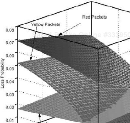
Figure 5.5. The loss probabilities of green-, yellow-, and red-marked packets in the AF1 class when using isolated trTCM.

Figure 5.6. The loss probabilities of green-, yellow-, and red-marked packets in the AF1 class when using interconnected trTCM.
For the reason mentioned in Section 5.4.2, drop probabilities for all BAs are derived and drawn in terms of the CIR, PIR, or TCA in average sending rates for the BAs, not in terms of TB sizes such as CBS and PBS in the TCA.
The proposed QoS mapping framework is evaluated by simulation in several steps. For video streaming, an error-resilient version of the ITU-T H.263+ stream is used and decoded by an error-robust video decoder. All other components are then simulated by NS [27].
We first investigate the VG functionality for dynamic feedforward QoS control with aggregated video flows. The network topology shown in Figure 5.7 is used to generate network dynamics. The network topology is simplified to elicit initial intuition out of the experiments. All sources travel through the same path, and there is no other traffic except the traffic from the sources. Each source transmits a video stream from the video trace. In each link of the DS domain in Figure 5.7, queuing with WFQ and multiple-RED is applied for link sharing of the scheduler and drop precedence of queue management. By giving different relative shares (relative to the average arrival rate) to different AF classes, the DS domain in this example provides relative differentiated services through “capacity differentiation” [113]. In this example, the class order from high to low is AF1, AF2, AF3, and BE.

Table 5.1. Network Load Condition for Performance Evaluation of Interconnected trTCM
Class Queue | Subscription Level (%) | Assigned Link BW by WFQ (kbps) | Imposed Load (kbps) |
|---|---|---|---|
AF1 | 136 | 1200 | 1632 |
AF2 | 123 | 900 | 1104 |
AF3 | 104 | 600 | 624 |
BE | N/A | 300 | 240 |
The main objective of the experiments in this section is to see the effectiveness of interconnected trTCM, so we do not use the static QoS mapping described in Section 3.4. Instead, a fixed DS level is assigned to an entire individual video flow. Several video flows with different DS levels are fed into interconnected trTCM. The test is designed to see the effectiveness of interconnected trTCM in preventing service inversion among multiple queue classes. Without interconnected trTCM, the packets in the highest class (AF1) may experience more delay than those in the lower class queues (e.g., AF2) if the higher class queue is overloaded. The reason is that isolated trTCM only changes the drop precedence within the class without downgrading the packet’s class.
To show the performance of interconnected trTCM, the experiments provide an unbalanced traffic load into the class queues, as specified in Table 5.1. The “imposed load” is designed so that the higher class has more loads. Three “Hall” (average rate per flow: 288 kbps) and two “Foreman” (384 kbps) video streams are assigned to the AF1 class queue; one “Foreman” and three “Akiyo” (240 kbps) streams are assigned to AF2; one “Foreman” and one “Akiyo” are assigned to AF3; and one “Akiyo” is assigned to BE. For all the flows assigned to the AF class, the color is set to green.
Note again that the higher class queues are deliberately loaded heavily (compared with the bandwidth portion assigned by the scheduler) to cause service inversion. This is done to demonstrate the promising regulation effect of interconnected trTCM under dynamic network load conditions.
Table 5.2. Performance Evaluation for Interconnected trTCM by Comparing Service Quality Parameters of Total Aggregated Flows in Each Class Queue
Without Interconnected trTCM | ||||
|---|---|---|---|---|
Flows in Class Queue | Achieved Throughput (kbps) | Packet Loss Rate (%) | Delay/Jitter (msec) | Re-Marking* Rate (%) |
AF1 | 1223.6 | 28.43 | 142.0/8.19 | 2.20 |
AF2 | 918.7 | 20.59 | 92.3/7.24 | 5.44 |
AF3 | 612.0 | 2.70 | 127.3/19.14 | 3.11 |
BE | 240 | 0.41 | 138.0/18.00 | 0 |
With Interconnected trTCM | ||||
|---|---|---|---|---|
Flows in Class Queue | Achieved Throughput (kbps) | Packet Loss Rate (%) | Delay/Jitter (msec) | Re-Marking** Rate (%) |
Note: * from the TB enforcement of each user; ** from traffic conditioning of interconnected trTCM. | ||||
AF1 | 1577.6 | 1.48 | 67.1/8.33 | 44.35 |
AF2 | 960.0 | 8.79 | 70.3/15.70 | 40.91 |
AF3 | 331.5 | 46.38 | 117.6/16.06 | 36.75 |
BE | 125.1 | 49.78 | 138.0/17.99 | 0 |
To give a complete explanation of Table 5.1, “subscription level” is defined to be 100*(imposed load/assigned link BW). Also, for this experiment, we set the trTCM’s PIR equal to the bandwidth assigned by the WFQ discipline, which is exercised at the border link.
The results in Table 5.2 show that the interconnected trTCM of the VG is useful for preventing service inversion. For example, for the case of “without interconnected trTCM,” a higher class has a higher packet loss rate, thus demonstrating service inversion. For the case of “with interconnected trTCM,” a higher class has a better (i.e., lower) packet loss rate. The same effect is shown for the delay/jitter measurements.
Table 5.2 also shows the rate of re-marking out of each class. The statistical analysis in Table 5.2 does not count the change of q value (re-marking) within the same AF class. As expected, with interconnected trTCM, much re-marking takes place when the high-class queue is overloaded. The re-marking shown for the case of “without interconnected trTCM” is not due to re-marking at its trTCM. Its tTCM does not re-mark across AF classes. The re-marking statistical analysis for the case of “without interconnected trTCM” is purely due to the per-flow traffic violation at the TB (downgrade to best-effort class), which is prior to the trTCM.
Next, with interconnected trTCM in place, we compare RPI-aware with RPI-blind mapping in a more realistic situation. In color-blind mapping, every packet prior to the interconnected trTCM, except for the one that violates the TB, is assigned q = 4 (AF23). RPI-aware mapping follows the guidelines in Section 3.4.2. In this experiment, we only use “Foreman” video streams, and in every trial of the experiment, only one stream uses RPI-blind mapping, which is used as a reference-to-be-compared stream (denoted by Fr). Different numbers of identical flows (all “Foreman”) with RPI-aware QoS mapping are used for different simulation runs, which results in different total traffic loads, as used for the horizontal axis of Figure 5.8. We then select one sample flow (denoted by Fs) from among the RPI-aware flows and compare its PSNR with that of RPI-blind Fr. (Due to symmetry, the PSNR of all the streams with RPI-aware mapping should be more or less the same.) For comparison, a “Foreman” video stream with the mapping guidance described in Section 3.4.2 is used to match the total cost constraint of the RPI-blind flow. Note that the loss rates of the compared flows can be different even though total cost remains the same, unless the loss rate of the DS level is exactly inverse-proportional to the cost of the corresponding DS level.

Figure 5.8. Performance comparison between RPI-blind and RPI-aware mapping over differently imposed network loads (end-to-end video PSNR performance).
Table 5.3. Comparison Between RPI-Blind and RPI-Aware Mapping over Different Imposed Loads (Packet Loss Rate and Throughput)
Imposed Load (%) | A Flow with RPI-Blind Mapping | A Flow with RPI-Aware Mapping | ||
|---|---|---|---|---|
Loss Rate (%) | Throughput (kbps) | Loss Rate (%) | Throughput (kbps) | |
< 100 | 0 | 384 | 0 | 384 |
102.4 | 2.16 | 370.79 | 4.98 | 366.7 |
108 | 5.25 | 357.46 | 9.18 | 349.87 |
115.2 | 8.57 | 340.66 | 13.71 | 332.57 |
123 | 13.2 | 321.77 | 22.3 | 300.34 |
As shown in Figure 5.8, the network load increases in accordance with the increasing number of RPI-aware flows for different simulations runs, and the overall PSNR for selected RPI-aware flows fs is degraded gracefully compared with that of the RPI-blind flow fr. Also, the RPI-blind flow experiences irregular end-to-end visual quality based on the load levels reflected in the average/standard deviation of average PSNR, where the vertical bar stands for the standard deviation. This implies that the higher k category packets of the RPI-blind flow cannot be protected properly, that they are sometimes lost more than lower k packets, and that the loss effect appears severe. In contrast, the RPI-aware mapping case protects the packets in accordance with the importance order k. The corresponding throughput and packet loss rate are provided in Table 5.3.
Moreover, let us observe the loss rate of fr and fs at the 115.2% load level from Table 5.3. The objective PSNR quality measure of fs is better than that of fr over all time, even though fs experiences a worse total packet loss rate, as shown in Figure 5.9. This is due to the fact that fs tends to lose relatively unimportant packets due to RPI-aware mapping.

Figure 5.9. PSNR comparison for RPI-blind and RPI-aware mappings for the “Foreman” sequence at 115.2% load.
In Figure 5.9, we show the loss rates of fs for different source categories. Recall that all k source categories of fr are mapped into q = AF23. With this cost constraint, fs is mapped as follows: k = 0 → AF32 with a loss rate of 33.3%; k= 1 ∼ 5 → AF31 with a loss rate of 30.5%; k = 6 ∼ 11 → AF23 with a loss rate of 8.66%; k = 12 ∼ 17 AF22 with a loss rate 1.42%; k = 18 → AF21 with no loss, and k = 19 → AF12 with no loss. Thus, the total loss rate of fs is 13.71%, while that of fr is 8.57%. The objective PSNR quality measure of fs is, however, better than that of fr over all time, even though fs experiences a worse total packet loss rate, as shown in Figure 5.9. It is again verified by the snapshots of the decoded video frame presented in Figure 5.10. RPI-aware mapping is a clear winner in the average or instance sense over time-varying network load conditions.

Finally, we verify the effectiveness of the proposed feedback QoS mapping control with RPI-aware mappings. With the other eight video flows of the “Foreman” sequence using RPI-aware mapping (i.e., total cost is equal to the mapping of all k to q = 4), one test “Foreman” video flow is compared in both cases: one case involves static DS mapping (i.e., all packets are mapped to q = 2), and the other case involves dynamic QoS mapping using the proposed feedback QoS mapping control. The k → q QoS per-flow mapping at the VG is adjusted based on periodic feedback from the receiver with a desired loss rate range. For this simulation, the range is set to [5, 15%], and we expect to get the average loss rate as the middle value (i.e., 10%) of this range. The results obtained illustrate how feedback QoS control affects the average loss rate dynamically. As shown in Figure 5.11, a VG can re-mark the DS level dynamically upon getting the receiver’s feedback. The average total loss rate of a reference case is 13.4%, and the loss rate of the feedback case is 9.5%, respectively. The time interval of QoS feedback and re-marking is 0.5 sec for both cases, and the time interval for the average loss rate calculation in Figure 5.11 (which appears on the next page) is the same.

This chapter discussed QoS mapping between categorized packet video and a proportional DiffServ network within a relative service differentiation framework. To show the performance of a VG, we set an encoded video stream as an example of streaming media in a simulated DiffServ network. Our previous works [118], [119] showed that QoS mapping between categorized packet video and the DS level can provide a gain in end-to-end video quality in terms of delay and loss under total cost constraint when using DiffServ. However, those works were limited to per-flow-based feedforward QoS mapping. This chapter extended them to full scope, using three layers of granularity (packetbased, session-based, and class-based) and feedback QoS mapping control. This process synthesized the two approaches to QoS mapping control: feed-forward and feedback. Extensive simulations were run to demonstrate the superior behavior of the proposed scheme. Our focus was on the QoS map-ping of unicast flows. How this may be generalized to multicast flows is still an open question.