
![]()
In most production environments, database and server optimization has long been the domain of DBAs. This includes server settings, hardware optimizations, index creation and maintenance, and many other responsibilities. SQL developers, however, are responsible for ensuring that their queries perform optimally. SQL Server is truly a developer’s DBMS, and as a result the developer responsibilities can overlap with those of the DBA. This overlap includes recommending database design and indexing strategies, troubleshooting poorly performing queries, and making other performance enhancement recommendations. In this chapter, we will discuss various tools and strategies for query optimization and performance enhancement and tuning the queries.
SQL Server Storage
SQL Server is designed to abstract away many of the logical and physical aspects of storage and data retrieval. In a perfect world, you wouldn’t have to worry about such things—you would be able to just “set it and forget it.” Unfortunately, the world is not perfect, and how SQL Server stores data can have a noticeable impact on query performance. Understanding SQL Server storage mechanisms is essential to properly troubleshooting performance issues. With that in mind, we’re going to give a brief overview of how SQL Server stores your data.
![]() Tip This section will give only a summarized description of how SQL Server stores data. The best detailed description of the SQL Server storage engine internals is in the book Inside Microsoft SQL Server 2012 Internals, by Kalen Delaney et al. (Microsoft Press, 2012).
Tip This section will give only a summarized description of how SQL Server stores data. The best detailed description of the SQL Server storage engine internals is in the book Inside Microsoft SQL Server 2012 Internals, by Kalen Delaney et al. (Microsoft Press, 2012).
SQL Server stores your databases in files. Each database consists of at least two files, a database file with an .mdf extension and a log file with an .ldf extension. You can also add additional files to a SQL Server database, normally with an .ndf extension.
Filegroups are logical groupings of files for administration and allocation purposes. By default, SQL Server creates all database files in a single primary filegroup. You can add additional filegroups to an existing database or specify additional filegroups at creation time. One of the big performance benefits of using multiple filegroups comes from placing the different filegroups on different physical drives. It’s common practice to increase performance by placing data files on a separate filegroup and physical drive from nonclustered indexes. It’s also common to place log files on a separate physical drive from both data and nonclustered indexes.
Understanding how physical separation of files improves performance requires an explanation of the read/write patterns involved with each type of information that SQL Server stores. Your actual database data will generally utilize a random access read/write pattern. The hard drive head is constantly repositioning itself to read and write user data to the database. Nonclustered indexes, likewise, are also usually random access in nature. The hard drive head repositions itself all over the place to traverse the nonclustered index. Once nodes that match the query criteria are found in the nonclustered index, if columns must be accessed that are not in the nonclustered index, the hard drive must again reposition itself to locate the actual data stored in the data file. The transaction log file has a completely different access pattern from both data and nonclustered indexes. SQL Server writes to the transaction log in a serial fashion. These conflicting access patterns can result in “head thrashing,” or constant repositioning of the hard drive head to read and write these different types of information.
Dividing your files by type and placing them on separate physical drives helps improve performance by reducing head thrashing and allowing SQL Server to perform I/O activities in parallel.
You can also place multiple data files in a single filegroup. When you create a database with multiple files in a single filegroup, SQL Server uses a proportional fill strategy across the files as data is added to the database. This means that SQL Server tries to fill all files in a filegroup at approximately the same time. Log files, which are not part of a filegroup, are filled using a serial strategy. If you add additional log files to a database, they will not be used until the current log file is filled.
![]() Tip You can move a table from its current filegroup to a new filegroup by dropping the current clustered index on the table and creating a new clustered index, specifying the new filegroup in the CREATE CLUSTERED INDEX statement.
Tip You can move a table from its current filegroup to a new filegroup by dropping the current clustered index on the table and creating a new clustered index, specifying the new filegroup in the CREATE CLUSTERED INDEX statement.
SQL Server uses a random access file to locate the data that reside in a specific location rather than reading the data from the beginning when reading the data. To enable the random access file, the system should have consistently sized allocation units in the file structure. SQL Server allocates space in the database in units called extents and pages to accomplish this. A page is an 8-KB block of contiguous storage. An extent consists of 8 logically contiguous pages, or 64 KB of storage. SQL Server has two types of extents: uniform extents, which are owned completely by a single database object, and mixed extents, which can be shared by up to eight different database objects. When a new table or index is created the pages are allocated from mixed extents. When the table or index grows beyond 8 pages, then the allocations are done in uniform extents to make the space allocation efficient.
This physical limitation on the size of pages is the reason for the historic limitations on data types such as varchar and nvarchar (up to 8,000 and 4,000 characters, respectively) and row size (8060 bytes). It’s also why special handling is required internally for LOB data types such as varchar(max), varbinary(max), and xml, since the data they contain can span many pages.
SQL Server keeps track of allocated extents with two types of allocation maps known as global allocation map (GAM) pages and shared global allocation map (SGAM) pages. GAM pages use bits to track all extents that have been allocated. SGAM pages use bits to track mixed extents with one or more free pages available. Index Allocation Map (IAM) tracks all the extents used by the index or table, and they are used to navigate through the data pages. Page Free Space (PFS) tracks the free space on each page that stores LOB values. The combination of the GAM and SGAM pages allows SQL Server to quickly allocate free extents, uniform/full mixed extents, and mixed extents with free pages as necessary whereas IAM and PFS are used to decide when the object needs the extent allocation.
The behavior of the SQL Server storage engine can have a direct bearing on performance. For instance, consider the code in Listing 18-1, which creates a table with narrow rows. Note that SQL Server can optimize storage for variable-length data types like varchar and nvarchar, so we’ve forced the issue by using fixed-length char data types for this example.
Listing 18-1. Creating a Narrow Table
CREATE TABLE dbo.SmallRows
(
    Id  int NOT NULL,
    LastName nchar(50) NOT NULL,
    FirstName nchar(50) NOT NULL,
    MiddleName nchar(50) NULL
);
INSERT  INTO  dbo.SmallRows
(
    Id,
    LastName,
    FirstName,
    MiddleName
)
SELECT
    BusinessEntityID,
    LastName,
    FirstName,
    MiddleName
FROM Person.Person;
The rows in the dbo.SmallRows table are 304 bytes wide. This means that SQL Server can fit about 25 rows on a single 8-KB page. You can verify this with the undocumented sys.fn_PhysLocFormatter function, as shown in Listing 18-2. Partial results are shown in Figure 18-1. The sys.fn_PhysLocFormatter function returns the physical locator in the form (fileipage:slot). As you can see in the figure, SQL Server fits 25 rows on each page (rows are numbered 0 to 24).
![]() Note The sys.fn_PhysLocFormatter function is undocumented and not supported by Microsoft. We’ve used it here for demonstration purposes, as it’s handy for looking at row allocations on pages; but don’t use it in production code.
Note The sys.fn_PhysLocFormatter function is undocumented and not supported by Microsoft. We’ve used it here for demonstration purposes, as it’s handy for looking at row allocations on pages; but don’t use it in production code.
Listing 18-2. Looking at Data Allocations for the SmallRows Table
SELECT
    sys.fn_PhysLocFormatter(%%physloc%%) AS [Row_Locator],
    Id
FROM dbo.SmallRows;
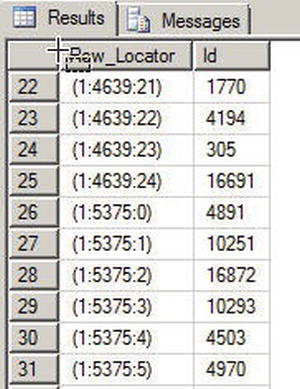
Figure 18-1. SQL Server Fits 25 Rows per Page for the dbo.SmallRows Table
By way of comparison, the code in Listing 18-3 creates a table with wide rows—3,604 bytes wide to be exact. The final SELECT query in Listing 18-3 retrieves the row locator information, demonstrating that SQL Server can only fit two rows per page for the dbo.LargeRows table. The results are shown in Figure 18-2.
Listing 18-3. Creating a Table with Wide Rows
CREATE TABLE dbo.LargeRows
(
    Id  int NOT NULL,
    LastName nchar(600) NOT NULL,
    FirstName nchar(600) NOT NULL,
    MiddleName nchar(600) NULL
);
INSERT  INTO  dbo.LargeRows
(
    Id,
    LastName,
    FirstName,
    MiddleName
)
SELECT
    BusinessEntityID,
    LastName,
    FirstName,
    MiddleName
FROM Person.Person;
SELECT
    sys.fn_PhysLocFormatter(%%physloc%%) AS [Row_Locator],
    Id
FROM dbo.LargeRows;
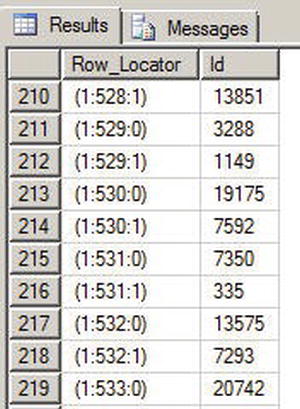
Figure 18-2. SQL Server Fits Only Two Rows per Page for the dbo.LargeRows Table
Now that we have created two tables with different row widths, the query in Listing 18-4 queries both tables with STATISTICS IO turned on to demonstrate the difference this makes to your I/O.
Listing 18-4. I/O Comparison of Narrow and Wide Tables
SET  STATISTICS IO ON;
SELECT
    Id,
    LastName,
    FirstName,
    MiddleName
FROM dbo.SmallRows;
SELECT
    Id,
    LastName,
    FirstName,
    MiddleName
FROM dbo.LargeRows;
The results returned, as shown following, demonstrate a significant difference in both logical reads and read-ahead reads:
(19972 row(s) affected)
Table ‘SmallRows’. Scan count 1, logical reads 799, physical reads 0, read-ahead reads 8, lob logical reads 0, lob physical reads 0, lob read-ahead reads 0.
(19972 row(s) affected)
Table ‘LargeRows’. Scan count 1, logical reads 9986, physical reads 0, read-ahead reads 10002, lob logical reads 0, lob physical reads 0, lob read-ahead reads 0.
The extra I/Os incurred by the query on the dbo.LargeRows table significantly affect the query plan estimated I/O cost. The query plan for the dbo.SmallRows query is shown in Figure 18-3, with an estimated I/O cost of 0.594315.
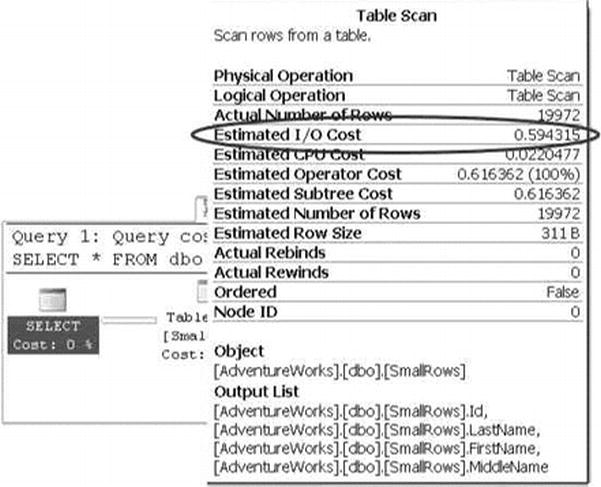
Figure 18-3. Estimated I/O Cost for the dbo.SmallRows Query
The query against the dbo.LargeRows table is significantly costlier with an estimated I/O cost of 7.39942—nearly 12.5 times greater than the dbo.SmallRows query. Figure 18-4 shows the higher cost for the dbo.LargeRows query.

Figure 18-4. Estimated I/O Cost for the dbo.LargeRows Query
As you can see from these simple examples, SQL Server has to read significantly more pages when a table is defined with wide rows. This increased I/O cost can cause a significant performance drain when performing SQL Server queries, even those queries that are otherwise highly optimized. One way to minimize the cost of I/O is to minimize the width of columns where possible, and always use the appropriate data type for the job. In the examples given, a variable-width character data type (varchar) would have significantly reduced the storage requirements of the sample tables. Although I/O cost is often a secondary consideration for developers and DBAs, and is often only addressed after slow queries begin to cause drag on a system, it’s a good idea to keep the cost of I/O in mind when initially designing your tables.
Partitioning the tables and indexes by range was introduced in SQL Server 2005. This functionality allows the data to be partitioned into rowsets based on the partitioning column value and the partitions can be placed into one more filegroups in the database to improve the performance of the query and manageability while treating them as a single object.
Partitioning is defined by a partition scheme which maps the partitions defined by the partition function to a set of files or filegroups that you define. The partition function specifies how the index or the table is partitioned. The column value that is used to define the partition can be of any data type except LOB data or timestamp. SQL Server 2008 supports 1,000 partitions by default and this meets most application needs; however there are cases where due to industry regulations you need to retain the daily data for more than 3 years and in those cases, we need the database to support more than 1,000 parititions. SQL Server 2008 R2 introduced the support for 15 K partitions; however, you need to run a stored procedure to enable this support. SQL Server 2012 provides support for 15,000 partitions by default and also provides native support for high availability and disaster recovery features such as AlwaysOn, replication, database mirroring, and log shipping as well.
Partitioning is useful to group the data from a large table into smaller chunks so that the data can be maintained independently for database operations such as speeding up queries, primarily with scans or loading data or reindexing to name a few. Partitioning can improve the query performance when the partitioning key is part of the query and the system has enough processors to process the query. Not all tables need to be partitioned; you should consider characteristics such as how large the table is, how it is being accessed and the query performance against the tables before considering whether to partition the data.
So, the first step to partitioning a table is to determine how the rows in the table will be divided between the partitions using a function called a partition function. To effectively design a partition function you need to specify logical boundaries. If you specify two boundaries, then three partitions are created and depending on whether the data is being partioned left or right the upper and lower boundary condition is set.
The partition function defines logical boundaries and the partition scheme defines the physical location, meaning filegroups, for them. Once the partition function is defined to set the logical boundary and the partition scheme is defined to map the logical boundary to filegroups, you can create the partitioned table. As with the table, you can partition the indexes as well. Partitioning the clustered index must have the partition key specified in the clustered index. Partitioning nonclustered index does not require the partition key; if the partition key is not specified, then SQL Server will include them in the indexes. The indexes that are defined with the partitioned tables can be aligned or nonaligned. The index is aligned if the table and the index logically have the same partition strategy.
In general, partitioning is most useful when the data has a time component. Generally large tables such as order details where most of the DML operations are performed on the current month’s data and previous months are simply used for selects may be good candidates to partition by month. This enables the queries to modify the data found in a single partition rather than scanning though the entire table to locate the data to be modified, hence enhancing the query performance.
Partitions can be split or merged easily in a sliding window scenario. Partitions can be split or merged only if all the indexes are aligned and the partition scheme and functions match. Partition alignment does not mean that both the objects have to use the same partition function, but if both objects have the same partition scheme, functions, and boundaries, they are considered to be aligned. When both the objects have the same partitioning scheme or file groups, they are storage aligned. Storage alignment can be physical or logical, and in both cases the performance of the queries is improved.
In addition to minimizing the width of columns by using the appropriate data type for the job, SQL Server 2012 provides built-in data compression functionality. By compressing your data directly in the database, SQL Server can reduce I/O contention and minimize storage requirements. There is some CPU overhead associated with compression and decompression of data during queries and DML activities, but data compression is particularly useful for historical data storage where access and manipulation demands are not as high as they might be for the most recent data. We will discuss the types of compression that SQL Server supports as well as the associated overhead and recommended usage of each.
Row Compression
SQL Server 2005 introduced an optimization to the storage format for the decimal data type in SP 2. The vardecimal type provided optimized variable-length storage for decimal data, which often resulted in significant space savings—particularly when your decimal columns contained a lot of zeros. This optimization is internal to the storage engine, so it’s completely transparent to developers and end users. In SQL Server 2008, this optimization was expanded to include all fixed-length numeric, date/time, and character data types in a feature known as row compression.
![]() Note The vardecimal compression options and SPs to manage this feature, including sp_db_vardecimal_storage_format and sp_estimated_rowsize_reduction_for_vardecimal, are deprecated, since SQL Server 2012 rolls this functionality up into the new row compression feature.
Note The vardecimal compression options and SPs to manage this feature, including sp_db_vardecimal_storage_format and sp_estimated_rowsize_reduction_for_vardecimal, are deprecated, since SQL Server 2012 rolls this functionality up into the new row compression feature.
SQL Server 2012 provides the useful sp_estimate_data_compression_savings procedure to estimate the savings you’ll get from applying compression to a table. Listing 18-5 estimates the space you’ll save by applying row compression to the Production.TransactionHistory table. This particular table contains fixed-length int, datetime, and money columns. The results are shown in Figure 18-5.
Listing 18-5. Estimating Row Compression Space Savings
EXEC sp_estimate_data_compression_savings 'Production',
    'TransactionHistory',
    NULL,
    NULL,
'ROW';

Figure 18-5. Row Compression Space Savings Estimate for a Table
![]() Note We changed the names of the last four columns in this example so they would fit in the image. The abbreviations are size_cur_cmp for Size with current compression setting (KB), size_req_cmp for Size with requested compression setting (KB), size_sample_cur_cmp for Sample size with current compression setting (KB), and size_sample_req_cmp for Sample size with requested compression setting (KB).
Note We changed the names of the last four columns in this example so they would fit in the image. The abbreviations are size_cur_cmp for Size with current compression setting (KB), size_req_cmp for Size with requested compression setting (KB), size_sample_cur_cmp for Sample size with current compression setting (KB), and size_sample_req_cmp for Sample size with requested compression setting (KB).
The results shown in Figure 18-5 indicate the current size of the clustered index (indexid = 1) is about 6.1 MB, while the two nonclustered indexes (indexid = 1 and 2) total about 2.9 MB. SQL Server estimates that it can compress this table down to a size of about 4.0 MB for the clustered index and 2.6 MB for the nonclustered indexes.
![]() Tip If your table does not have a clustered index, the heap is indicated in the results with an index_id of 0.
Tip If your table does not have a clustered index, the heap is indicated in the results with an index_id of 0.
You can turn row compression on for a table with the DATACOMPRESSION = ROW option of the CREATE TABLE and ALTER TABLE DDL statements. Listing 18-6 turns on row compression for the Production.TransactionHistory table.
Listing 18-6. Turning on Row Compression for a Table
ALTER TABLE Production.TransactionHistory REBUILD
WITH (DATA_COMPRESSION  =  ROW);
You can verify that the ALTER TABLE statement has applied row compression to your table with the sp_spaceused procedure, as shown in Listing 18-7. The results are shown in Figure 18-6.
Listing 18-7. Viewing Space Used by a Table after Applying Row Compression
EXEC sp_spaceused N'Production.TransactionHistory';

Figure 18-6. Space Used by the Table after Applying Row Compression
As you can see in the figure, the size of the data used by the Production.TransactionHistory table has dropped to about 4.0 MB. The indexes are not automatically compressed by the ALTER TABLE statement. To compress the nonclustered indexes, you need to issue ALTER INDEX statements with the DATA_COMPRESSION = ROW option. You can use the DATACOMPRESSION = NONE option to turn off row compression for a table or index.
Row compression uses variable-length formats to store your fixed-length data, and SQL Server stores an offset value in each record for every variable-length value it stores. Prior to SQL Server 2008, this offset value was fixed at 2 bytes of overhead per variable-length value. SQL Server 2008 introduced a new record format that uses a 4-bit offset for variable-length columns that are 8 bytes in length or less.
SQL Server 2012 also has the capability to compress data at the page level using two methods: column-prefix compression and page-dictionary compression. Where row compression is good for minimizing the storage requirements for highly unique fixed-length data at the row level, page compression helps minimize the storage space required by duplicated data stored in pages.
The column-prefix compression method looks for repeated prefixes in columns of data stored on a page. Figure 18-7 shows a sample page from a table with repeated prefixes in columns underlined.

Figure 18-7. Page with Repeated Column Prefixes Identified
To compress the column prefixes identified in Figure 18-7, SQL Server creates an anchor record. This is a row in the table just like any other row, except that it serves the special purpose of storing the longest value in the column containing a duplicated column prefix. The anchor record is later used by the storage engine to re-create the full representations of the compressed column values when they are accessed. This special type of record is accessible only internally by the storage engine and cannot be retrieved or modified directly by normal queries or DML operations. Figure 18-8 shows the column prefix-compressed version of the page from Figure 18-7.
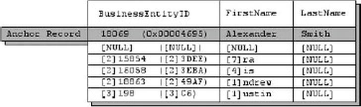
Figure 18-8. Page with Column-Prefix Compression Applied
There are several items of note in the column prefix-compressed page shown in Figure 18-8. First is that the anchor record has been added to the page. Column-prefix compression uses byte patterns to indicate prefixes, making the column-prefix method data type-agnostic. In this instance, the BusinessEntityID column is an int data type, but as you can see it takes advantage of data type compression as well. We’ve shown the BusinessEntityID column values in both int and varbinary format to demonstrate that they are compressed as well.
The next interesting feature of column-prefix compression is that SQL Server replaces the prefix of each column with an indicator of how many bytes need to be prepended from the anchor record value to re-create the original value. NULL is used to indicate that the value in the table is actually the full anchor record value.
![]() Note The storage engine uses metadata associated with each value to indicate the difference between an actual NULL in the column and a NULL indicating a placeholder for the anchor record value.
Note The storage engine uses metadata associated with each value to indicate the difference between an actual NULL in the column and a NULL indicating a placeholder for the anchor record value.
In the example given, each column of the first row is replaced with NULLs that act as placeholders for the full anchor record values. The second row’s BusinessEntityID column indicates that the first two bytes of the value should be replaced with the first two bytes of the BusinessEntitylD anchor record column. The FirstName column of this row indicates that the first seven bytes of the value should be replaced with the first seven bytes of the FirstName anchor record column, and so on.
Page-dictionary compression is the second type of compression that SQL Server uses to compress pages. Page-dictionary compression creates an on-page dictionary of values that occur multiple times across any columns and rows on the page. It then replaces those duplicate values with indexes into the dictionary. Consider Figure 18-9, which shows a data page with duplicate values.

Figure 18-9. Uncompressed Page with Duplicate Values across Columns and Rows
The duplicate valuesArthur and Martin are added to the dictionary and replaced in the data page with indexes into the dictionary. The value Martin is replaced with the index value (0) everywhere it occurs in the data page, and the value Arthur is replaced with the index value (1). This is demonstrated in Figure 18-10.

Figure 18-10. Page Compressed with Page-dictionary Compression
When SQL Server performs page compression on data pages and leaf index pages, it first applies row compression, and then it applies page-dictionary compression.
![]() Note For performance reasons, SQL Server does not apply page-dictionary compression to non-leaf index pages.
Note For performance reasons, SQL Server does not apply page-dictionary compression to non-leaf index pages.
You can estimate the savings you’ll get through page compression with the sp_estimate_data_compression_savings procedure, as shown in Listing 18-8. The results are shown in Figure 18-11.
Listing 18-8. Estimating Data Compression Savings with Page Compression
EXEC  sp_estimate_data_compression_savings 'Person',
    'Person',
    NULL,
    NULL,
'PAGE';

Figure 18-11. Page Compression Space Savings Estimate
As you can see in Figure 18-11, SQL Server estimates that it can use page compression to compress the Person.Person table from 29.8 MB in size down to about 18.2 MB, a considerable savings. You can apply page compression to a table with the ALTER TABLE statement, as shown in Listing 18-9.
Listing 18-9. Applying Page Compression to the Person.Person Table
ALTER TABLE Person.Person REBUILD
WITH (DATA_COMPRESSION = PAGE);
As with row compression, you can use the sp_spaceused procedure to verify how much space page compression saved you.
Page compression is great for saving space, but it does not come without a cost. Specifically you pay for the space savings with increased CPU overhead for SELECT queries and DML statements. So when should you use page compression? Microsoft makes the following recommendations:
- If the table or index is small in size, then the overhead you incur from compression will probably not be worth the extra CPU overhead.
- If the table or index is heavily accessed for queries and DML actions, the extra CPU overhead can significantly impact your performance. It’s important to identify usage patterns when deciding whether or not to compress the table or index.
- Use the sp_estimate_data_compression_savings procedure to estimate the space savings. If the estimated space savings is insignificant (or nonexistent), then the extra CPU overhead will probably outweigh the benefits.
In addition to row compression and page compression, SQL Server provides sparse columns, which let you optimize NULL value storage in columns. The trade-off (and you knew there would be one) is that the cost of storing non-NULL values goes up by 4 bytes for each value. Microsoft recommends using sparse columns when it will result in at least 20 to 40 percent space savings. For an int column, for instance, at least 64 percent of the values must be NULL to achieve a 40 percent space savings with sparse columns. Sparse column is a column attribute that provides storage optimization, meaning when NULL values are stored in the column it takes up 0 bytes.
To demonstrate sparse columns in action, we’ll use a query that generates columns with a lot of NULLs in them. The query shown in Listing 18-10 creates a pivot-style report that lists the CustomerID numbers associated with every sales order down the right-hand side of the results, and a selection of product names from the sales orders. The intersection of each CustomerID and product name contains the number of each item ordered by each customer. A NULL indicates that a customer did not order an item. Partial results of this query are shown in Figure 18-12.
Listing 18-10. Pivot Query that Generates Columns with Many NULLs
SELECT
    CustomerID,
    [HL Road Frame - Black, 58],
    [HL Road Frame - Red, 58],
    [HL Road Frame - Red, 62],
    [HL Road Frame - Red, 44],
    [HL Road Frame - Red, 48],
    [HL Road Frame - Red, 52],
    [HL Road Frame - Red, 56],
    [LL Road Frame - Black, 58]
FROM
(
    SELECT soh.CustomerID, p.Name AS ProductName,
        COUNT
        (
        CASE  WHEN  sod.LineTotal  IS  NULL  THEN  NULL
        ELSE 1
        END
        )  AS  NumberOfItems
        FROM Sales.SalesOrderHeader soh
        INNER JOIN Sales.SalesOrderDetail sod
        ON soh.SalesOrderID  =  sod.SalesOrderID
        INNER JOIN Production.Product p
        ON  sod.ProductID  =  p.ProductID
        GROUP BY
        soh.CustomerID,
        sod.ProductID,
        p.Name
)  src
PIVOT
(
    SUM(NumberOfItems) FOR ProductName
    IN
    (
    "HL Road Frame - Black, 58",
    "HL  Road  Frame  -  Red, 58",
    "HL  Road  Frame  -  Red, 62",
    "HL  Road  Frame  -  Red, 44",
    "HL  Road  Frame  -  Red, 48",
    "HL  Road  Frame  -  Red, 52",
    "HL  Road  Frame  -  Red, 56",
    "LL Road Frame - Black, 58"
    )
)  AS  pvt;
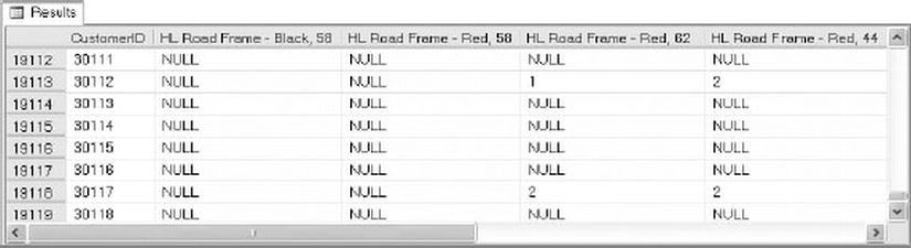
Figure 18-12. Pivot Query that Returns the Number of Each Item Ordered by Each Customer
Listing 18-11 creates two similar tables to hold the results generated by the query in Listing 18-10. The tables generated by the CREATE TABLE statements in Listing 18-11 have the same structure, except that the SparseTable includes the keyword SPARSE in its column declarations, indicating that these are sparse columns.
Listing 18-11. Creating Sparse and Nonsparse Tables
CREATE TABLE NonSparseTable
(
    CustomerID int NOT NULL PRIMARY KEY,
    "HL Road Frame - Black, 58" int NULL,
    "HL  Road  Frame  -  Red,  58"  int NULL,
    "HL  Road  Frame  -  Red,  62"  int NULL,
    "HL  Road  Frame  -  Red,  44"  int NULL,
    "HL  Road  Frame  -  Red,  48"  int NULL,
    "HL  Road  Frame  -  Red,  52"  int NULL,
    "HL  Road  Frame  -  Red,  56"  int NULL,
    "LL Road Frame - Black, 58" int NULL
);
CREATE  TABLE  SparseTable
(
    CustomerID int NOT NULL PRIMARY KEY,
    "HL  Road  Frame  -  Black,  58"  int  SPARSE  NULL,
    "HL  Road  Frame  -  Red,  58"  int  SPARSE NULL,
    "HL  Road  Frame  -  Red,  62"  int  SPARSE NULL,
    "HL  Road  Frame  -  Red,  44"  int  SPARSE NULL,
    "HL  Road  Frame  -  Red,  48"  int  SPARSE NULL,
    "HL  Road  Frame  -  Red,  52"  int  SPARSE NULL,
    "HL  Road  Frame  -  Red,  56"  int  SPARSE NULL,
    "LL  Road  Frame  -  Black,  58"  int  SPARSE  NULL
);
After using the query in Listing 18-10 to populate these two tables, you can use the sp_spaceused procedure to see the space savings that sparse columns provide. Listing 18-12 executes sp_spaceused on these two tables, both of which contain identical data. The results shown in Figure 18-13 demonstrate that the SparseTable takes up only about 25 percent of the space used by the NonSparseTable since NULL values in sparse columns take up no storage space.
Listing 18-12. Calculating the Space Savings of Sparse Columns
EXEC sp_spaceused N'NonSparseTable';
EXEC sp_spaceused N'SparseTable';

Figure 18-13. Space Savings Provided by Sparse Columns
Sparse Column Sets
In addition to sparse columns, SQL Server provides support for XML sparse column sets. An XML column set is defined as an xml data type column, and it contains non-NULL sparse column data from the table. An XML sparse column set is declared using the COLUMNSET FOR ALLSPARSECOLUMNS option on an xml column. As a simple example, the AdventureWorks Production.Product table contains several products that do not have associated size, color, or other descriptive information. Listing 18-13 creates a table called Production.SparseProduct that defines several sparse columns and a sparse column set.
Listing 18-13. Creating and Populating a Table with a Sparse Column Set
CREATE TABLE Production.SparseProduct
(
    ProductID int NOT NULL PRIMARY KEY,
    Name  dbo.Name  NOT  NULL,
    ProductNumber nvarchar(25) NOT NULL,
    Color nvarchar(15) SPARSE NULL,
    Size  nvarchar(5)  SPARSE  NULL,
    SizeUnitMeasureCode nchar(3) SPARSE NULL,
    WeightUnitMeasureCode nchar(3) SPARSE NULL,
    Weight decimal(8, 2) SPARSE NULL,
    Class nchar(2) SPARSE NULL,
    Style nchar(2) SPARSE NULL,
    SellStartDate datetime NOT NULL,
    SellEndDate datetime SPARSE NULL,
    DiscontinuedDate datetime SPARSE NULL,
    SparseColumnSet xml COLUMN_SET FOR ALL_SPARSE_COLUMNS
);
GO
INSERT INTO Production.SparseProduct
(
    ProductID,
    Name,
    ProductNumber,
    Color,
    Size,
    SizeUnitMeasureCode,
    WeightUnitMeasureCode,
    Weight,
    Class,
    Style,
    SellStartDate,
    SellEndDate,
    DiscontinuedDate
)
SELECT
    ProductID,
    Name,
    ProductNumber,
    Color,
    Size,
    SizeUnitMeasureCode,
    WeightUnitMeasureCode,
    Weight,
    Class,
    Style,
    SellStartDate,
    SellEndDate,
    DiscontinuedDate
FROM  Production.Product;
GO
You can view the sparse column set in XML form with a query like the one in Listing 18-14. The results in Figure 18-14 show that the first five products do not have any sparse column data associated with them, so the sparse column data takes up no space. By contrast, products 317 and 318 both have Color and Class data associated with them.
Listing 18-14. Querying XML Sparse Column Set as XML
SELECT TOP(7)
ProductID,
SparseColumnSet FROM Production.SparseProduct;
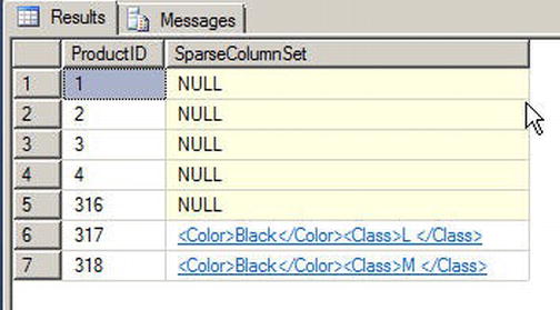
Figure 18-14. Viewing Sparse Column Sets in XML Format
Although SQL Server manages sparse column sets using XML, you don’t need to know XML to access sparse column set data. In fact, you can access the columns defined in sparse column sets using the same query and DML statements you’ve always used, as shown in Listing 18-15. The results of this query are shown in Figure 18-15.
Listing 18-15. Querying Sparse Column Sets by Name
SELECT
    ProductID,
    Name,
    ProductNumber,
    SellStartDate,
    Color,
    Class
FROM  Production.SparseProduct
WHERE ProductID IN (1, 317);
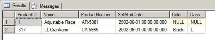
Figure 18-15. Querying Sparse Column Sets with SELECT Queries
Sparse column sets provide the benefits of sparse columns, with NULLs taking up no storage space at all. However, the downside is that non-NULL sparse columns that are a part of a column set are stored in XML format, adding some storage overhead as compared with their nonsparse, non-NULL counterparts.
Indexes
Your query performance may begin to lag over time for several reasons. It may be that database usage patterns have changed significantly over time, or the amount of data stored in the database has increased significantly over time, or the database has fallen out of maintenance. Whatever the reason, the knee-jerk reaction of many developers and DBAs is to throw indexes at the problem. While indexes are indeed useful for increasing performance, they do consume resources, both in storage and maintenance. Before creating new indexes all over your database, it’s important to understand how they work. In this section, we will give an overview of SQL Server’s indexing mechanisms.
In SQL Server parlance, a heap is simply an unordered collection of data pages with no clustered index. SQL Server uses index allocation map (IAM) pages to track allocation units of the following types:
- Heap or B-tree (a.k.a. “hobt”) allocation units, which track storage allocation for tables and indexes
- LOB allocation units, which track storage allocation for LOB data
- Small LOB (SLOB) allocation units, which track storage allocation for row overflow data
As any DBA will tell you, a table scan, which is SQL Server’s “brute force” data retrieval method, is a bad thing (though not necessarily the worst thing that can happen). In a table scan, SQL Server literally scans every data page that was allocated by the heap. Any query against the heap causes a table scan operation. To determine which pages have been allocated for the heap, SQL Server must refer back to the IAM. A table scan is known as an allocation order scan since it uses the IAM to scan the data pages in the order in which they were allocated by SQL Server.
Heaps are also subject to fragmentation, and the only way to eliminate fragmentation from the heap is to copy the heap to a new table or create a clustered index on the table or performing periodic maintenance to keep the index from being fragmented. Forward pointers introduce another performance-related issue to heaps. When a row with variable length column is updated with row length larger than the page size, the updated row may have to be moved to a new page. When SQL Server must move the row in a heap to a new location, it leaves a forward pointer to the new location at the old location. If the row is moved again, SQL Server leaves another forward pointer, and so on. Forward pointers result in additional I/Os, making table scans even less efficient (and you thought it wasn’t possible!).
Table scans are not essentially bad if you have to perform row based operations or if you are querying against tables with small data sets such as lookup tables, where adding an index creates maintenance overhead.
![]() Tip Querying a heap with no clustered or nonclustered indexes always results in a costly table scan.
Tip Querying a heap with no clustered or nonclustered indexes always results in a costly table scan.
Clustered Indexes
If a heap is an unordered collection of data pages, how do you impose order on the heap? The answer is a clustered index. A clustered index turns an unordered heap into a collection of data pages ordered by the specified clustered index columns. Clustered indexes are managed in the database as B-tree structures.
The top level of the clustered index B-tree is known as the root node, the bottom level nodes are known as leaf nodes, and all nodes in between the root node and leaf nodes are collectively referred to as intermediate nodes. In a clustered index, the leaf nodes contain the actual data rows for a table, and all leaf nodes point to the next and previous leaf nodes, forming a doubly linked list. The clustered index holds a special position in SQL Server indexing because its leaf nodes contain the actual table data. Since the page chain for the data pages can be ordered only one way, there can only be one clustered index defined per table. The query optimizer uses the clustered index for seeks, because the data can be found directly at the leaf level if a clustered index is used. The clustered index B-tree structure is shown in Figure 18-16.
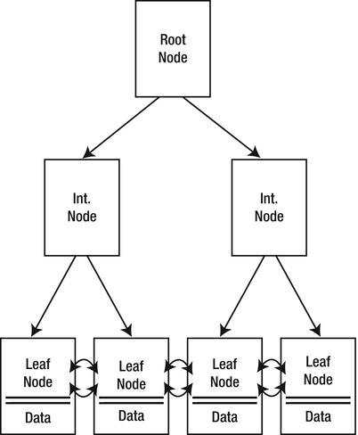
Figure 18-16. Clustered Index B-tree Structure
GUARANTEED ORDER
Despite the fact that the data pages in a clustered index are ordered by the clustered index columns, you cannot depend on table rows being returned in clustered index order unless you specify an ORDER BY clause in your queries. There are a couple of reasons for this, including the following:
- Your query may join multiple tables and the optimizer may choose to return results in another order based on indexes on another table.
- The optimizer may use an allocation order scan of your clustered index, which will return results in the order in which data pages were allocated.
The bottom line is that the SQL query optimizer may decide that, for whatever reason, it is more efficient to return results unordered or in an order other than clustered index order. Because of this, you can’t depend on results always being returned in the same order without an explicit ORDER BY clause. We’ve seen many cases of developers being bitten because their client-side code expected results in a specific order, and after months of receiving results in the correct order, the optimizer decided that returning results in a different order would be more efficient. Don’t fall victim to this false optimism—use ORDER BY when ordered results are important.
Many are under the impression that a clustered index scan is the same thing as a table scan. In one sense they are correct—when SQL Server performs an unordered clustered index scan, it refers back to the IAM to scan the data pages of the clustered index using an allocation order scan, just like a table scan.
However, SQL Server has another option for clustered indexes, the ordered clustered index scan. In an ordered clustered index scan, or leaf-level scan, SQL Server can follow the doubly linked list at the leaf node level instead of referring back to the IAM. The leaf-level scan has the benefit of scanning in clustered index order. Table scans do not have the option of a leaf-level scan since the leaf-level pages are not ordered or linked. Clustered indexes also eliminate the performance problems associated with forward pointers in the heap, although you do have to pay attention to fragmentation, page splits, and fill factor when you have a clustered index on your table. Fill factor determines how many rows can be filled in the index page. When the index page is full and new rows need to be inserted, SQL Server will create a new index page and transfer rows to the new page from the previous page which is called as page split. The page splits can be reduced by setting the proper fill factor to determine how much free space there is in the index pages.
So when should you use a clustered index? As a general rule, we like to put a clustered index on nearly every table we create although it is not a requriement to have clustered indexes for all the tables. Although you will have to decide on which columns you wish to create in your clustered indexes, here are some general recommendations for columns to consider in your clustered index design:
- Columns that provide a high degree of uniqueness. Monotonically increasing columns, such as IDENTITY or SEQUENCE columns, are ideal as they also reduce the overhead associated with page splits that result from insert and update operations.
- Columns that return a range of values using operators like >=, <, and BETWEEN. When you use a range query on clustered index columns, after the first match is found, the remaining values are guaranteed to be linked/adjacent in the B-tree.
- Columns that are used in queries that return large result sets of data from those columns.
- Columns that are used in the ON clause of a JOIN. Usually, these are primary key or foreign key columns. SQL Server creates a unique clustered index on the column when the primary key is added to the table.
- Columns that are used in GROUP BY or ORDER BY clauses. A clustered index on these columns can help SQL Server improve performance when ordering query result sets.
You should also make your clustered indexes as narrow as possible (often a single int or uniqueidentifier column), since this decreases the number of levels that must be traversed and hence reduces I/O. Another reason is that they are automatically appended to all nonclustered indexes on the same table as row locators, so keeping the clustered index key small will reduce the size of nonclustered indexes as well.
Nonclustered Indexes
Nonclustered indexes provide another tool for indexing relational data in SQL Server. Like clustered indexes, SQL Server stores nonclustered indexes as B-tree structures. Unlike clustered indexes, however, each leaf node in a nonclustered index contains the nonclustered key value and a row locator. The table rows are stored apart from the nonclustered index—in the clustered index if there is one defined on the table or in a heap if the table has no clustered index. Figure 18-17 shows the nonclustered index B-tree structure. Recall from the previous section on Clustered Indexes that data rows can only be stored in one sorted order and this is achieved via a clustered index. Order can only be achieved via the clustered index.
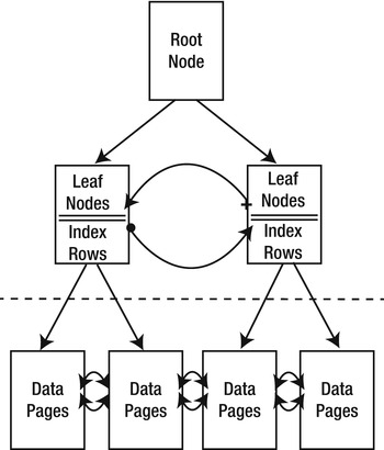
Figure 18-17. Nonclustered Index B-tree Structure
If a table has a clustered index, all nonclustered indexes defined on the table automatically include the clustered index columns as the row locator. If the table is a heap, SQL Server creates row locators to the rows from the combination of the file identifier, page number, and slot on the page. Therefore, if you add a clustered index at a later date, be aware that you will need to rebuild your non-clustered indexes to use the clustered index column as row locator rather than file identifier.
Nonclustered indexes are associated with the RID lookup and key lookup operations. RID lookups are bookmark lookups into the heap using row identifiers (RIDs), while key lookups are bookmark lookups on tables with clustered indexes. Once SQL Server locates the index rows that fulfill a query, if the query requires more columns than the nonclustered index covers, then the query engine must use the row locator to find the rows in the clustered index or the heap to retrieve necessary data. These are the operations referred to as a RID and key lookups, and they are costly operations—so costly, in fact, that many performance-tuning operations are based on eliminating them.
![]() Note In prior versions of SQL Server, we had the bookmark lookup operation. In SQL Server 2012, this operation has been split into two distinct operations, the RID lookup and the key lookup, to differentiate between bookmark lookups against heaps and clustered indexes.
Note In prior versions of SQL Server, we had the bookmark lookup operation. In SQL Server 2012, this operation has been split into two distinct operations, the RID lookup and the key lookup, to differentiate between bookmark lookups against heaps and clustered indexes.
One method of dealing with RID and key lookups is to create covering indexes. A covering index is a nonclustered index that contains all of the columns necessary to fulfill a given query or set of queries. If a nonclustered index does not cover a query, for each row, SQL Server has to look up the row to retrieve values for the columns that are not included in the nonclustered index. By performing the lookup using RID there is extra I/O for each row in the resultset. Whereas, when you define a covering index, the query engine can determine that all the information it needs to fulfill the query is stored in the nonclustered index rows, so it does not need to perform a lookup operation.
SQL Server offers the option to INCLUDE columns in the index. An included column is not an index key, so it allows the columns to appear on the leaf pages of the nonclustered index and hence improve the query performance.
![]() Tip Prolific author and SQL Server MVP Adam Machanic defines a clustered index as a covering index for every possible query against a table. This definition provides a good tool for demonstrating that there’s not much difference between clustered and nonclustered indexes, and it helps to reinforce the concept of index covering.
Tip Prolific author and SQL Server MVP Adam Machanic defines a clustered index as a covering index for every possible query against a table. This definition provides a good tool for demonstrating that there’s not much difference between clustered and nonclustered indexes, and it helps to reinforce the concept of index covering.
The sample query in Listing 18-16 shows a simple query against the Person.Person table that requires a bookmark lookup, which is itself shown in the query plan in Figure 18-18.
Listing 18-16. Query Requiring a Bookmark Lookup
SELECT
BusinessEntityID,
LastName,
FirstName,
MiddleName,
Title FROM Person.Person WHERE LastName = N'Duffy';
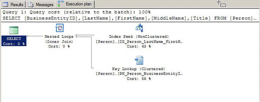
Figure 18-18. Bookmark Lookup in the Query Plan
So why is there a bookmark lookup (referenced as a key lookup operator in the query plan)? The answer lies in the query. This particular query uses the LastName column in the WHERE clause to limit results, so the query engine decides to use the IX_Person_LastName_FirstName_MiddleName nonclustered index to fulfill the query. This nonclustered index contains the LastName, FirstName, and MiddleName columns, as well as the BusinessEntityID column, which is defined as the clustered index. The lookup operation is required because the SELECT clause also specifies that the Title column needs to be returned in the result set. Since the Title column is not included in the covering index, SQL Server has to refer back to the table’s data pages to retrieve it.
Creating an index with the Title column included in the nonclustered index as shown in Listing 18-17 removes the lookup operation from the query plan for the query in Listing 18-16. As shown in Figure 18-19, the IX_Covering_Person_LastName_FirstName_MiddleName index covers the query.

Figure 18-19. The Covering Index Eliminates the Lookup Operation
![]() Tip Another alternative to eliminate this costly lookup operation is to modify the nonclustered index used in the example to include the Title column, which would create a covering index for the query.
Tip Another alternative to eliminate this costly lookup operation is to modify the nonclustered index used in the example to include the Title column, which would create a covering index for the query.
Listing 18-17. Query Using a Covering Index
CREATE NONCLUSTERED INDEX [IX_Covering_Person_LastName_FirstName_MiddleName] ON [Person].[Person]
(
     [LastName] ASC,
     [FirstName] ASC,
     [MiddleName] ASC
) INCLUDE (Title)
WITH (PAD_INDEX = OFF, STATISTICS_NORECOMPUTE = OFF, SORT_IN_TEMPDB = OFF, DROP_EXISTING = OFF, ONLINE = OFF, ALLOW_ROW_LOCKS = ON, ALLOW_PAGE_LOCKS = ON) ON [PRIMARY]
GO
You can define up to 999 nonclustered indexes per table. You should carefully plan your indexing strategy and try to minimize the number of indexes you define on a single table. Nonclustered indexes can require a substantial amount of additional storage, and there is a definite overhead involved in automatically updating them whenever the table data changes. When deciding how many indexes to add to a table, consider the usage patterns carefully. Tables with data that does not change—or rarely changes—may derive greater benefit from having lots of indexes defined on them than tables whose data is modified often.
Nonclustered indexes are useful for the following types of queries:
- Queries that return one row, or a few rows, with high selectivity.
- Queries that can use an index with high selectivity (generally above 95 percent). Selectivity is a measure of the unique key values in an index. SQL Server will often ignore indexes with low selectivity.
- Queries that return small ranges of data that would otherwise result in a clustered index or table scan. These types of queries often use simple equality predicates (=) in the WHERE clause.
- Queries that are completely covered by the nonclustered index.
In SQL Server 2012, filtered indexes provide a way to create more targeted indexes that require less storage and can support more efficient queries. Filtered indexes are optimized nonclustered indexes that allow you to easily add filtering criteria to restrict the rows included in the index with a WHERE clause. A filtered index improves the performance of queries since the index is smaller than a nonclustered index and the statistics are more accurate since they cover only the rows in the filered index. Adding a filtered index to the table where a nonclustered index is unnecessary reduces disk storage for the nonclustered index and the statistics update the cost as well. Listing 18-18 creates a filtered index on the Size column of the Production.Product table that excludes NULL.
Listing 18-18. Creating and Testing a Filtered Index on the Production.Product Table
CREATE NONCLUSTERED INDEX IX_Product_Size
ON Production.Product
(
Size,
SizeUnitMeasureCode )
WHERE Size IS NOT NULL;
GO
SELECT
ProductID,
Size,
SizeUnitMeasureCode FROM Production.Product WHERE Size  =  'L';
GO
![]() Tip Filtered indexes are particularly well suited for indexing non-NULL values of sparse columns.
Tip Filtered indexes are particularly well suited for indexing non-NULL values of sparse columns.
Optimizing Queries
One of the more interesting tasks that SQL developers and DBAs must perform is optimizing queries. To borrow an old cliché, query optimization is as much art as science. There are a lot of moving parts within the SQL query engine, and your task is to give the optimizer as much good information as you can so that it can make good decisions at runtime.
Performance is generally measured in terms of response time and throughput, defined as follows:
- Response time is the time that it takes for SQL Server to complete a task, such as a query.
- Throughput is a measure of the volume of work that SQL Server can complete in a fixed period of time, such as the number of transactions per minute.
There are several other factors that affect your overall system performance but are outside the scope of this book. Application responsiveness, for instance, depends on several additional factors like network latency and UI architecture, both of which are beyond SQL Server’s control. In this section, we will talk about how to use query plans to diagnose performance issues.
When you submit a T-SQL script or statement to the SQL Server query engine, SQL Server compiles your code into a query plan. The query plan is composed of a series of physical and logical operators that the optimizer has chosen to complete your query. The optimizer bases its choice of operators on a wide array of factors like data distribution statistics, cardinality of tables, and availability of useful indexes. SQL Server uses a cost based optimizer, meaning the execution plan it chooses will have the lowest estimated cost.
SQL Server can return query plans in a variety of formats. Our preference is the graphical query execution plan, which we’ve used in examples throughout the book. Figure 18-20 shows a query plan for a simple query that joins two tables.

Figure 18-20. Query Execution Plan for an Inner Join Query
You can generate a graphical query plan for a given query by selecting the Query ![]() Include Actual Execution Plan option from the SSMS menu, and then running your SQL statements. Alternatively, you can select Query
Include Actual Execution Plan option from the SSMS menu, and then running your SQL statements. Alternatively, you can select Query ![]() Display Estimated Execution Plan without running the query.
Display Estimated Execution Plan without running the query.
A graphical query plan is read from right to left and top to bottom. It contains arrows indicating the flow of data through the query plan. The arrows show the relative amount of data being moved from one operator to the next, with wider arrows indicating larger numbers of rows, as shown in Figure 18-20. You can position the mouse pointer on top of any operator or arrow in the graphical query plan to display a pop-up with additional information about the operator or data flow between operators, such as the number of rows being acted upon and the estimated row size. You can also right-click an operator or arrow and select Properties from the pop-up menu to view even more descriptive information.
You can also right-click in the Execution Plan window and select Save Execution Plan As to save your graphical execution plan as an XML query plan. Query plans are saved with a .sqlplan file extension and can be viewed in graphical format in SSMS by double-clicking the file. This is particularly useful for troubleshooting queries remotely, since your users or other developers can save the graphical query plan and e-mail it to you, and you can open it up in a local instance of SSMS for further investigation.
ACTUAL OR ESTIMATED?
Estimated execution plans are useful in determining the optimizer’s intent. The word estimated in the name can be a bit misleading since all query plans are based on the optimizer’s estimates of your data distribution, table cardinality, and more.
There are some differences between estimated and actual query plans, however. Since an actual query plan is generated as your T-SQL statements are executed, the optimizer can add additional information to the query plan as it runs. This additional information includes items like actual rebinds and rewinds, values that return the number of times init() method is called in the plan and actual number of rows. When dealing with temporary objects, actual query plans have better information available concerning which operators are being used as well. Consider the following simple script that creates, populates, and queries a temporary table:
CREATE TABLE #tl (
BusinessEntityID int NOT NULL,
LastName nvarchar(50),
FirstName nvarchar(50),
MiddleName nvarchar(50) );
CREATE INDEX tl_LastName ON #tl (LastName);
INSERT INTO #tl (
BusinessEntityID,
LastName,
FirstName,
MiddleName )
SELECT
BusinessEntityID,
LastName,
FirstName,
MiddleName FROM Person.Person;
SELECT
BusinessEntityID,
LastName,
FirstName,
MiddleName FROM #tl WHERE LastName = N'Duffy';
DROP TABLE #tl;
In the estimated query plan for this code, the optimizer indicates that it will use a table scan, as shown following, to fulfill the SELECT query at the end of the script:

The actual query plan, however, uses a much more efficient nonclustered index seek with a bookmark lookup operation to retrieve the two relevant rows from the table, as shown here:

The difference between the estimated and actual query plans in this case is the information available at the time the query plan is generated. When the estimated query plan is created, there is no temporary table and no index on the temporary table, so the optimizer guesses that a table scan will be required. When the actual query plan is generated, the temporary table and its nonclustered index both exist, so the optimizer comes up with a better query plan.
In addition to graphical query plans, SQL Server supports XML query plans and text query plans, and it can report additional runtime statistics. This additional information can be accessed using the statements shown in Table 18-1.
Table 18-1. Query Plan Generation Statements
| Statement | Description |
|---|---|
| SET SHOWPLAN_ALL ON/OFF | Returns a text-based estimated execution plan without executing the query |
| SET SHOWPLAN_TEXT ON/OFF | Returns a text-based estimated execution plan without executing the query |
| SET SHOWPLAN_XML ON/OFF | Returns an XML-based estimated execution plan without executing the query |
| SET STATISTICS IO ON/OFF | Returns statistics information about logical I/O operations during execution of a query |
| SET STATISTICS PROFILE ON/OFF | Returns actual query execution plans in result sets following the result set generated by each query executed |
| SET STATISTICS TIME ON/OFF | Returns statistics about the time required to parse, compile, and execute statements at runtime |
Once the query is compiled, it can be executed and the execution need not necessarily happen after the query is compiled. So, if the query is executed several days after it has been compiled, the underlying data might have changed and the plan that has been compiled may not be optimal during the execution time. So, when this query is being executed SQL Server first checks to see if the plan is still valid. If the query optimizer decides that the plan is suboptimal, a few statements or the entire batch will be recompiled to produce a different plan. These compilations are called recompilations and although sometimes it is necessary to recompile the queries, this process can slow down the query or batch executions considerably, and so it is optimal to reduce recompilations.
Some of the causes for recompilations are:
- Schema changes such as adding or dropping columns, constraints, indexes, statistics, etc.
- Running sp_recompile on stored procedure or trigger.
- Using Set options after the batch has started such as ANSI_NULL_DFLT_OFF, ANSI_NULLS, ARITHABORT, etc.
One of the main causes for excessive recompilations is the use of temporay tables in the queries. If you create a temporary table in StoredProcA and reference the temporary table in a statement in StoredProcB, then the statement must be recompiled every time StoredProcA runs. Table variable may be a good option to replace a temporary table for a small number of rows.
Sometimes you see suboptimal query performance, and there are few causes for this. One of the common causes is using nonSearch ARGumentable (nonSARGable) expressions in the where clauses or joins which prevents SQL Server from using the index. Using these expressions can slow down the queries significantly as well. Some of the nonSARGable expressions are inequality expression comparisions, functions, implicit datatype conversions, and the LIKE keyword. Often these expresions can be rewritten to use an index. Consider a simple script below that finds person names starting with ‘C.’
SELECT Title, FirstName, LastName FROM person.person WHERE SUBSTRING(FirstName, 1,1) = 'C'
The above query will cause a table scan, whereas if the query is rewritten as follows, the optimizer will use clustered seek if a proper index exists in the table, hence improving performance.
SELECT Title, FirstName, LastName FROM person.person WHERE FirstName LIKE 'C%'
Sometimes you do have to use functions in the queries for calculations, and in these cases if you replace the function with an indexed computed column then the SQL Server query optimizer can generate a plan that will use an index. SQL Server can match an expression to the computed column to use statistics; however, the expression should match the computed column definition exactly.
Methodology
The methodology that has served us well when troubleshooting performance issues involves the following eight steps:
- Recognize the issue: Before you can troubleshoot a performance issue, you must first determine that there is an actual issue. The recognition of an issue can begin with something as simple as end users complaining that their applications are running slowly.
- Identify the source: Once you’ve recognized that there is an issue, you need to identify the problem as an SQL Server-related problem. For instance, if you receive reports of database-enabled applications running slowly, it’s important to narrow down the source of the problem. If the issue is a network bandwidth or latency issue, for instance, it can’t be resolved through simple query optimizations. If it’s a T-SQL issue, you can use tools like SQL Profiler and query plans to identify the problematic code.
- Review baseline: Once you have identified the issue and the source, evaluate the baseline. For instance, if the end user is complaining that the application runs slowly, you need to understand the definition of slow and also if it is reproducible. Slow could mean the reports are not rendered within 1 minute or slow could mean that the reports are not rendered within 10 milliseconds. Without a proper baseline you have nothing to compare to and cannot really acertain if the issue exists or not.
- Analyze the code: Once you’ve identified T-SQL code as the source of the problem, it’s time to dig deeper and analyze the root cause of the problem. The operators returned in graphical query plans provide an excellent indicator of the source of many problems. For example, you may spot a costly clustered index scan operator where you expected a more efficient nonclustered index seek.
- Define possible solutions: After the issues have been identified in the code, it’s time to come up with potential solutions. If bookmark lookup operations are slowing down your query performance, for instance, you may determine that adding a new nonclustered index or modifying an existing one is a possible fix for the issue. Another possible solution might be changing the query to return fewer columns that are already covered by an index.
- Evaluate the solutions: A critical step after defining your possible solutions is to evaluate the practicality of those solutions. Many things affect whether or not a solution is practical. For instance, you may be forbidden to change indexes on the production servers, in which case adding or modifying indexes to solve an issue may be impractical. On the other hand, your client applications may depend on all of the columns currently being returned in the query’s result sets, so changing the query to return fewer columns may not be a workable solution.
During this step of the process, you also need to determine the impact of your solutions on other parts of the system. Adding or modifying an index on the server to solve a query performance problem might fix the problem for a single query, but it might introduce new performance problems for other queries or DML statements. These conflicting needs should be evaluated. - Implement the solution: This step of the process is where you actually apply your solution. You will most likely have a subprocess here, in which you apply the solution first to a development environment, and then to a quality assurance (QA) environment, and finally promote it to the production environment.
- Examine the impact of the solution: After implementing your solution, you should revisit it to ensure that it actually fixes the problem. This is a very important step that many people largely ignore, only revisiting their solutions when another issue occurs. By scheduling to revisit your solution, you can take a proactive approach and head off problems before they affect your end users.
Scalability is another important factor to consider when writing T-SQL. Scalability is a measure of how well your code works under increasing demands. For instance, a query may provide acceptable performance when the source table contains 100,000 rows and 10 end users simultaneously querying. However, the same query may suffer performance problems when the table grows to 1,000,000 rows and the number of end users grows to 100. Increasing stress on a system tends to uncover scalability and performance issues that weren’t previously apparent in your code base. As pressure on your database grows, it’s important to monitor changing access patterns and increasing demands on the system to proactively handle issues before they affect end users.
It’s important to also understand when an issue is not really a problem, or at least not one that requires a great deal of attention. As a general rule, we like to apply the 80/20 rule when optimizing queries. That is to say, as a rule of thumb, focus your efforts on optimizing the 20 percent of code that is executed 80 percent of the time. If you have an SP that takes a long time to execute but is only run once a day, and a second procedure that takes a significant amount of time but is run 10,000 times a day, you’d be well served to focus your efforts on the latter procedure.
Your main goal in designing and writing the application is to enable the users get accurate resultsets in an efficient way. So, when you come across a performance issue, the first place to start with is the actual query itself. For any given session, the query or the thread can be in one of two states: it is either running or it is waiting on something. When the query is running it could be compiling or executing; and when the query is waiting, it can be waiting for I/O, Network, Memory, Locks or Latches, etc., or it can be forced to wait to make sure the process yields for other processes. Whatever the case may be, when the query is waiting on the resource SQL Server logs the wait type for the resource the query is waiting on. You can then use this information to understand why the query performance is affected.
To better help you understand the resource usage, there are three performance metrics that can play role in the query performace—CPU, Duration, and Logical Reads. CPU is essentially the worker time spent to execute the query; Duration is the time the worker thread takes to execute the query, which also includes the time it takes to wait for the resources as well as time it takes to execute the query; and Logical Reads are the number of data pages read by the query execution from the buffer pool or the memory. If the page does not exist in the buffer pool then SQL Server performs a physical read to read the page into the buffer pool. Since we are measuring the performance on the query, logical reads are considered to measure the performance and not physical reads. The wait time can be simply calculated by the formula Duration-CPU.
Waitstats is one of the methodologies that will help you identify opportunities to tune the query performance, and SQL Server 2012 has 649 wait types. Let’s say in your application you have some users read from the table and some users write to the same table as well. At any given time, if rows are being inserted into the table, the query that is trying to read those rows has to stop processing since the resource is unavailable. Once the row insertion is completed, the read process gets a signal that the resource is available now for this process, and once a scheduler is available to process the read thread, the query is processed. The time SQL Server spends to acquire the system resource in this example is called a wait. The time SQL Server spends waiting for the process to be signed when the resource is available is called resource wait time. Once the process is signaled the process has to wait for the scheduler to be available for the process to continue, and this wait time is called signal wait time. Both resource wait time and signal wait time combined together gives the wait time in milliseconds.
The wait types can be queried using DMVs sys.dm_os_waiting_tasks and sys.dm_os_wait_stats and sys.dm_exec_requests. sys.dm_os_waiting_tasks and sys.dm_exec_requests return the details on what the tasks are waiting on currently, whereas sys.dm_os_wait_stats lists the aggregate of the waits since the instance has been last restarted, So, you need to check the sys.dm_os_waiting_tasks for the query performance analysis.
Let’s review how waits can help you tune queries with a common example. You might have come across the situation where you are trying to insert a set of rows to the table and the insert process hangs and is not responsive. When you query sp_who2, it does not show any blocking; however, the insert process waits for a long time before it completes. Let’s see how we can use waitstats to debug this scenario. Listing 18-19 is the script that inserts rows to the waitsdemo table we created in Adventureworks with user session id 54.
Listing 18-19. Script to Demonstrate Waits
use adventureworks
go
CREATE TABLE [dbo].[waitsdemo](
       [Id] [int] NOT NULL,
       [LastName] [nchar](600) NOT NULL,
       [FirstName] [nchar](600) NOT NULL,
       [MiddleName] [nchar](600) NULL
) ON [PRIMARY]
GO
declare @id int  =  1
while (@id <  = 50000)
begin
 insert into waitsdemo
 	select @id,'Foo', 'User',NULL
 SET @id  =  @id  +  1
end
Now, to identify the issue of why the insert query is being blocked, let’s query the DMVs sys.dm_exec_requests and sys.dm_exec_sessions to see the processes that are currently executing and also query the DMC sys.dm_os_waiting_tasks to see the list of processes that are currently waiting. The DMV queries are listed in Listing 18-20 and partial results are shown in Figure 18-21. In our example, the insert query using session id 54 is waiting on the shrinkdatabase task with session id 98.
Listing 18-20. DMV to Query Current Processes and Waiting Tasks
--List waiting user requests
SELECT
er.session_id, er.wait_type, er.wait_time,
er.wait_resource, er.last_wait_type,
er.command,et.text,er.blocking_session_id
FROM sys.dm_exec_requests AS er
JOIN sys.dm_exec_sessions AS es
ON es.session_id  =  er.session_id
AND es.is_user_process  =  1
CROSS APPLY sys.dm_exec_sql_text(er.sql_handle) AS et
GO
--List waiting user tasks
SELECT
wt.waiting_task_address, wt.session_id, wt.wait_type,
wt.wait_duration_ms, wt.resource_description
FROM sys.dm_os_waiting_tasks AS wt
JOIN sys.dm_exec_sessions AS es
ON wt.session_id  =  es.session_id
AND es.is_user_process  =  1
GO
-- List user tasks
SELECT
t.session_id, t.request_id, t.exec_context_id,
t.scheduler_id, t.task_address,
t.parent_task_address
FROM sys.dm_os_tasks AS t
JOIN sys.dm_exec_sessions AS es
ON t.session_id  =  es.session_id
AND es.is_user_process  =  1
GO

Figure 18-21. Results of sys.dm_os_waiting_tasks
The above results show that process 54 is indeed waiting and the wait type is writelog which means that the I/O to the log files is slow. When you correlate this to the session_id 98 which is shrinkdatabase task, you can identify that the root cause for the performance issue with the insert query is the shrinkdatabase process. Once the shrinkdatabase operation completes the insert query starts to process as shown in Figure 18-22.

Figure 18-22. Results of DMV to Show the Blocking Thread
Not all wait types need to be monitored constantly. Some of the wait types like broker_*, clr_* can be ignored if you are not using service broker or CLR in your datbases. We have only touched the tip of the iceberg with this example, waits can be a much more powerful mechanism in helping to identify and resolve query performance issues.
Extended Events
Extended Events (XEvents) is a diagnostic system that can help you troubleshoot performance problems with the SQL Server. It was first introduced in SQL 2008 and then went through a complete makeover in SQL Server 2012 with additional event types and new user interface and templates similar to SQL Server Profiler. Let’s review the Extended Events user interface first and then use a case to see how we can troubleshoot with Extended Events. The XEvents user interface is integrated with Management Studio, and there is a separate node in the tree called Extended Events. To start a new Extended Events session, expand the Management node and then expand Extended Events. Right click Sessions and then click New Session. Figure 18-23 shows the Extended Events user interface.
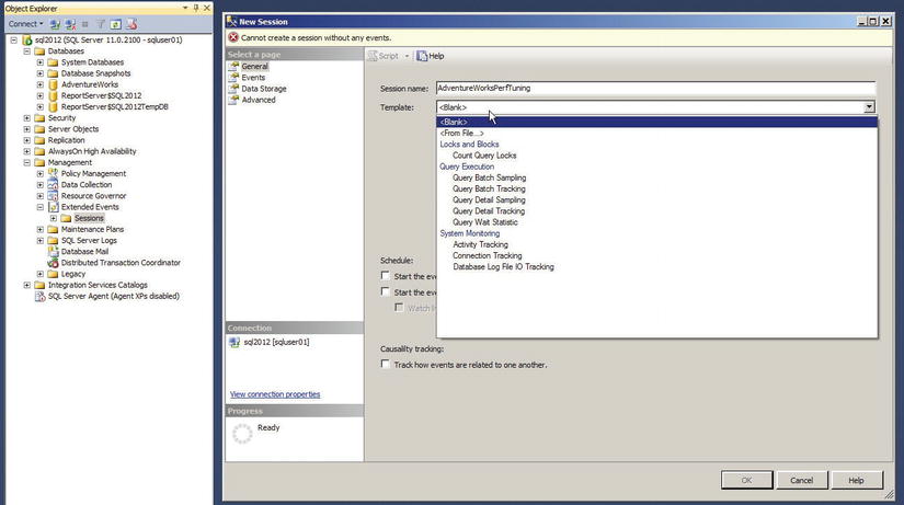
Figure 18-23. Extended Events New Session
XEvents offers a rich diagnostic framework that is highly scalable and offers the capability to collect little or large amounts of data in order to troubleshoot a given performance issue. XEvents has the same capabilities as SQL Profiler, and so you may ask why should you use XEvents and not SQL Profiler. Anybody who has worked with SQL Server can tell you that SQL Profiler adds significant resource overhead when tracing the server, which can sometimes bring the server to its knees. The reason for the overhead with SQL Profiler is that when you use SQL Profiler to trace the activities on the server, all the events are streamed to the client and the events are filtered based on the criteria set by you on the client side, which needs lot of resources to process the events. Whereas, with XEvents, the filtering happens on the server side, so the events that are needed are not sent to the client—hence better performance with a process that is less chatty. Another reason to start using XEvents is simply because SQL Profiler has been marked for deprecation.
Extended events sessions can be based on predefined templates or you can create the session by choosing specific events. You can also autostart an XEvents session on server startup, one of the features that is not available in SQL Profiler. Figure 18-24 shows the autostart option.
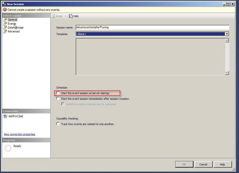
Figure 18-24. Object Explorer Database Table Pop-up Context Menu
The Event library lists all the events that are searchable as well, and they are categorized and grouped based on the events. You are able to search the events based on names and/or descriptions. Once you select the events you want to track, you are able to set the filter criteria. After the filters have been defined, you can select the fields you want to track. The common fields that are tracked are selected by default. Figure 18-25 shows a sample session to capture the SQL statements for performance tuning.

Figure 18-25. Sample Extended Events Session Configuration for SQL Performance Tuning
Once all of the criteria have been defined, you can set the target depending on what you want to do with the data, whether you want to capture the data to a file, forward it to in-memory targets, or write it to a live reader. Figure 18-26 shows the possible targets for the session.
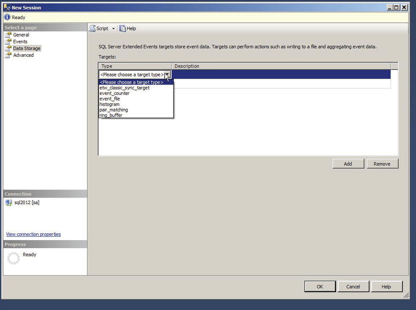
Figure 18-26. Extended Events Target Type
Figure 18-27 shows the results of the Extended Events streaming the live data of the SQL statements for the performance tuning session.

Figure 18-27. Sample Data from the Extended Events Session for SQL Performance Tuning
Now let’s take a common problem: a business user is complaining that the application is slow and there is a lot of blocking. You need to figure out where the problem is, given the application is third-party software. The challenge is to identify a piece of application functionality and the queries behind this functionality that are causing the performance issue. So you have multiple areas to investigate, including clients, network, blocking, CPU, and I/O issues. One way to approach the problem is to run the tool Performance Monitor (perfmon) and start a profiler trace, and try to tie in the application issue to the server metrics, but there is no direct way to get the details on the query chain of the lead blocker that causes and follows the blocking issue without using XEvents.
If the application is built on the latest ODBC drivers or the new ADO.NET 4.5, the application is going to attach an identifier called ConnectionId which is a guide to the server when the connections are made which makes the process of tracing or correlating activities between client and server much simpler. Along with this, the client will send another identifier called ActivityId which provides information on the process that is currently executing. With the ConnectionId and ActivityId we will now have the information required to build a complete image of the activities that take place in the server, and we can effectively trace it with the server activities to identify the bottlenecks.
Extended Events makes common problems like page splits or locking much easier to identify and resolve with proper code changes. For tracking page splits, you can set up an Extended Events session using a script as shown in Listing 18-21.
Listing 18-21. Extended Event Session Script to Troubleshoot Login Timeouts
CREATE EVENT SESSION [Troubleshoot page split] ON SERVER
ADD EVENT sqlserver.page_split(

ACTION(sqlserver.client_app_name,sqlserver.database_id,sqlserver.database_name,sqlserver.plan_
handle,sqlserver.server_instance_name,sqlserver.server_principal_
name,sqlserver.server_principal_sid,sqlserver.session_id,sqlserver.session_nt_username,sqlserver.sql_text,sqlserver.transaction_
id,sqlserver.username)),
ADD EVENT sqlserver.rpc_completed(

ACTION(sqlserver.client_app_name,sqlserver.database_id,sqlserver.database_name,sqlserver.plan_
handle,sqlserver.server_instance_name,sqlserver.server_principal_
name,sqlserver.server_principal_sid,sqlserver.session_id,sqlserver.session_nt_username,sqlserver.sql_text,sqlserver.transaction_
id,sqlserver.username)),
ADD EVENT sqlserver.rpc_starting(

ACTION(sqlserver.client_app_name,sqlserver.database_id,sqlserver.database_name,sqlserver.plan_
handle,sqlserver.server_instance_name,sqlserver.server_principal_
name,sqlserver.server_principal_sid,sqlserver.session_id,sqlserver.session_nt_username,sqlserver.sql_text,sqlserver.transaction_
id,sqlserver.username)),
ADD EVENT sqlserver.sp_statement_completed(

ACTION(sqlserver.client_app_name,sqlserver.database_id,sqlserver.database_name,sqlserver.plan_
handle,sqlserver.server_instance_name,sqlserver.server_principal_
name,sqlserver.server_principal_sid,sqlserver.session_id,sqlserver.session_nt_username,sqlserver.sql_text,sqlserver.transaction_
id,sqlserver.username)),
ADD EVENT sqlserver.sp_statement_starting(

ACTION(sqlserver.client_app_name,sqlserver.database_id,sqlserver.database_name,sqlserver.plan_
handle,sqlserver.server_instance_name,sqlserver.server_principal_name,sqlserver.server_principal_
sid,sqlserver.session_id,sqlserver.session_nt_username,sqlserver.sql_text,sqlserver.transaction_
id,sqlserver.username))
ADD TARGET package0.event_file(SET filename  =  N'C:TempTroubleshoot page split.xel')
WITH (MAX_MEMORY  =  4096 KB,EVENT_RETENTION_MODE  =  ALLOW_SINGLE_EVENT_LOSS,MAX_DISPATCH_LATENCY  =  30 SECONDS,MAX_EVENT_SIZE  =  0
KB,MEMORY_PARTITION_MODE  =  NONE,TRACK_CAUSALITY  =  OFF,STARTUP_STATE  =  OFF)
GO
Now you can start the Extended Events session that was created using Listing 18-21and start identifying the queries and the session details that cause these page splits. This will help you narrow down the issue very quickly and troubleshoot what is causing the page splits.
Summary
SQL Server stores data in 8-KB pages that it allocates in contiguous groups of 8 pages each, which are known as extents. In a perfect world, SQL Server’s logical and physical storage mechanisms would not make a difference to you as a developer. In the real world, however, an understanding of storage engine operation is important to maximizing performance. We began this chapter with an overview of the SQL Server storage engine and how it affects performance.
Indexes are the primary means of increasing query performance on SQL Server. We continued the discussion by addressing the concepts of heaps, clustered indexes, and nonclustered indexes, with details of how each affects the overall performance of your queries and DML statements.
Optimizing queries depends on maximizing two critical aspects: response time and throughput. SQL Server provides query plans and statistics, in addition to other external tools, to help diagnose performance issues. We wrapped up this chapter with a suggested methodology for dealing with performance issues. Using a methodology like the eight-step process described here will help you quickly narrow down the source of performance issues; define, evaluate, and implement solutions; and take a proactive approach in addressing future performance-related issues.
Using troubleshooting techniques such as waitstats and DMVs will help you narrow down the performance issues and will provide you information to derive a complete picture of what is going on in the system. Combining this with high performance event monitoring infrastructure such as Extended Events provides proactive monitoring capabilities for the servers that allow you to identify issues and resolve them in timely fashion.
We hope that you’ve enjoyed reading this book as much as we’ve enjoyed bringing it to you. We wish you all the best in your T-SQL development efforts, and we hope you find this book helpful in your development endeavors.
EXERCISES
1. [Choose all that apply] SQL Server 2012 uses which of the following types of files to store database information:
a. Data files (.mdf extension)
b. Transaction log files (.ldf extension)
c. Additional data files (.ndf extension)
d. Rich text files (.rtf extension)
2. [True/False] SQL Server stores data in 8-KB storage units known as pages.
3. [Choose one] Eight contiguous 8-KB pages of storage in SQL Server are known as which of the following:
a. A filegroup
b. A chunk
c. An extent
d. A file
4. [Fill in the blank] A heap is an _________ collection of data pages.
5. [Fill in the blank] Clustered indexes and nonclustered indexes are managed by SQL Server as _______________ structures.
6. [Fill in the blank] _______________ sessions can be used to trace waits.
7. [Fill in the blank] Optimized nonclustered index is _________________.
8. [Choose all that apply] SQL Server performance is measured using which of the following terms:
a. Throughput
b. Luminescence
c. Response time
d. All of the above