
![]()
Common Table Expressions and Windowing Functions
SQL Server 2012 continues support for the extremely useful common table expression (CTE), first introduced in SQL Server 2005. CTEs can simplify your queries to make them more readable and maintainable. SQL Server also supports self-referential CTEs, which make for very powerful recursive queries.
In addition, SQL Server supports windowing functions, which allow you to partition your results and apply numbering and ranking values to the rows in the result set partitions. This chapter begins with a discussion of the power and benefits of CTEs and finishes with a discussion of SQL Server windowing functions.
Common Table Expressions
CTEs are a powerful addition to SQL Server. A CTE is more like temporary table that generates a named result set that exists only during the life of a single query or DML statement or until they are explicitly dropped. A CTE is built in the same code line as the SELECT statement or the DML statement that uses it, whereas creating and using a temporary table is usually a two-step process. CTEs offer several benefits over derived tables and views, including the following:
- CTEs are transient, existing only for the life of a single query or DML statement. This means that you don’t have create them as permanent database objects like views.
- A single CTE can be referenced multiple times by name in a single query or DML statement, making your code more manageable. Derived tables have to be rewritten in their entirety every place they are referenced.
- CTEs can be used to enable grouping by columns that are derived from a scalar subset or a function that is not deterministic.
- CTEs can be self-referencing, providing a powerful recursion mechanism.
- Queries referencing a CTE can be used to define a cursor.
CTEs can range in complexity from extremely simple to highly elaborate constructs. All CTEs begin with the WITH keyword followed by the name of the CTE and a list of the columns it returns. This is followed by the AS keyword and the body of the CTE which is the associated query or DML statement with semicolon as terminator for multistatement batch. Listing 8-1 is a very simple example of a CTE designed to show the basic syntax.
Listing 8-1. Simple CTE
WITH GetNamesCTE (
BusinessEntityID,
FirstName,
MiddleName,
LastName )
AS (
SELECT
BusinessEntityID, FirstName, MiddleName, LastName
FROM Person.Person ) SELECT
BusinessEntityID,
FirstName,
MiddleName,
LastName FROM GetNamesCTE
;
In Listing 8-1, the CTE is defined with the name GetNamesCTE and returns columns named BusinessEntityID, FirstName, MiddleName, and LastName. The CTE body consists of a simple SELECT statement from the AdventureWorks 2012 Person.Person table. The CTE has an associated SELECT statement immediately following it. The SELECT statement references the CTE in its FROM clause.
WITH OVERLOADED
The WITH keyword is overloaded in SQL Server, meaning that it’s used in many different ways for many different purposes in T-SQL. It’s used to specify additional options in DDL CREATE statements, to add table hints to queries and DML statements, and to declare XML namespaces when used in the WITH XMLNAMESPACES clause, just to name a few. Now it’s also used as the keyword that indicates the beginning of a CTE definition. Because of this, whenever a CTE is not the first statement in a batch, the statement preceding it must end with a semicolon. This is one reason why we strongly recommend using the statement-terminating semicolon throughout your code.
Simple CTEs have some restrictions on their definition and declaration:
- A CTE must be followed by single INSERT, DELETE, UPDATE or SELECT statement.
- All columns returned by a CTE must have a unique name. If all of the columns returned by the query in the CTE body have unique names, you can leave the column list out of the CTE declaration.
- A CTE can reference other previously defined CTEs in the same WITH clause, but cannot reference CTEs defined after the current CTE (known as a forward reference).
- You cannot use the following keywords, clauses, and options within a CTE: COMPUTE, COMPUTE BY, FOR BROWSE, INTO, and OPTION (query hint). Also, you cannot use ORDER BY unless you specify the TOP clause.
- Multiple CTEs can be defined in a nonrecursive CTE and all the definitions must be combined by one these set operators: UNION ALL, UNION, INTERSECT or EXCEPT
- As we mentioned in the “WITH Overloaded” sidebar, when a CTE is not the first statement in a batch, the preceding statement must end with a semicolon statement terminator.
Keep these restrictions in mind when you create CTEs.
Multiple Common Table Expressions
You can define multiple CTEs for a single query or DML statement by separating your CTE definitions with commas. The main reason for doing this is to simplify your code to make it easier to read and manage. CTEs provide a means of visually splitting your code into smaller functional blocks, making it easier to develop and debug. Listing 8-2 demonstrates a query with multiple CTEs, with the second CTE referencing the first. Results are shown in Figure 8-1.
Listing 8-2. Multiple CTEs
WITH GetNamesCTE (
BusinessEntityID,
FirstName,
MiddleName,
LastName )
AS (
SELECT
BusinessEntityID, FirstName, MiddleName, LastName
FROM Person.Person ),
GetContactCTE (
BusinessEntityID,
FirstName,

MiddleName, LastName, Email, HomePhoneNumber
)
AS ( SELECT gn.BusinessEntityID, gn.FirstName, gn.MiddleName, gn.LastName, ea.EmailAddress, pp.PhoneNumber FROM GetNamesCTE gn LEFT JOIN Person.EmailAddress ea
ON gn.BusinessEntityID = ea.BusinessEntityID LEFT JOIN Person.PersonPhone pp ON gn.BusinessEntityID = pp.BusinessEntityID AND pp.PhoneNumberTypeID = 2 )
SELECT BusinessEntityID, FirstName, MiddleName, LastName, Email,
HomePhoneNumber FROM GetContactCTE;

Figure 8-1. Partial results of a query with multiple CTEs
CTE READABILITY BENEFITS
You can use CTEs to make your queries more readable than equivalent query designs that utilize nested subqueries. To demonstrate, the following query uses nested subqueries to return the same result as the CTE-based query in Listing 8-2.
The sample in Listing 8-2 contains two CTEs, named GetNamesCTE and GetContactCTE. The GetNamesCTE is borrowed from Listing 8-1; it simply retrieves the names from the Person.Person table.
WITH GetNamesCTE ( BusinessEntityID, FirstName, MiddleName, LastName )
AS ( SELECT
BusinessEntityID, FirstName, MiddleName, LastName FROM Person.Person )
The second CTE, GetContactCTE, joins the results of GetNamesCTE to the Person. EmailAddress table and the Person.PersonPhone tables:
GetContactCTE (BusinessEntityID, FirstName, MiddleName, LastName, Email,
HomePhoneNumber )
AS ( SELECT gn. BusinessEntityID, gn.FirstName, gn.MiddleName, gn.LastName, ea.EmailAddress, pp.PhoneNumber FROM GetNamesCTE gn LEFT JOIN Person.EmailAddress ea
ON gn. BusinessEntityID = ea. BusinessEntityID LEFT JOIN Person.PersonPhone pp ON gn. BusinessEntityID = pp. BusinessEntityID AND pp.PhoneNumberTypelD = 2 )
Notice that the WITH keyword is only used once at the beginning of the entire statement. The second CTE declaration is separated from the first by a comma, and does not accept the WITH keyword. Finally, notice how simple and readable the SELECT query associated with the CTEs becomes when the joins are moved into CTEs.
SELECT
BusinessEntityID,
FirstName,
MiddleName,
LastName,
EmailAddress,
HomePhoneNumber FROM GetContactCTE;
![]() Tip You can reference a CTE from within the body of another CTE or from the associated query or DML statement. Both types of CTE references are shown in Listing 8-2—the GetNamesCTE is referenced by the GetContactCTE and the GetContactCTE is referenced in the query associated with the CTEs.
Tip You can reference a CTE from within the body of another CTE or from the associated query or DML statement. Both types of CTE references are shown in Listing 8-2—the GetNamesCTE is referenced by the GetContactCTE and the GetContactCTE is referenced in the query associated with the CTEs.
Recursive Common Table Expressions
A recursive CTE is the one where the initial CTE is executed repeatedly to return the subset of the data until the complete resultset is returened. CTEs can reference themselves in the body of the CTE, is a powerful feature for querying hierarchical data stored in the adjacency list model. Recursive CTEs are similar to nonrecursive CTEs, except that the body of the CTE consists of multiple sets of queries that generate result sets with multiple rows unioned together with the UNION ALL set operator. At least one of the queries in the body of the recursive CTE must not reference the CTE; this query is known as the anchor query. Recursive CTEs also contain one or more recursive queries that reference the CTE. These recursive queries are unioned together with the anchor query (or queries) in the body of the CTE. Recursive CTEs require a top-level UNION ALL operator to union the recursive and nonrecursive queries together. Multiple anchor queries may be unioned together with INTERSECT, EXCEPT, or UNION operators, while multiple recursive queries can be unioned together with UNION ALL. The recursion stops when there are no rows returned from the previous query. Listing 8-3 is a simple recursive CTE that retrieves a result set consisting of the numbers 1 through 10.
Listing 8-3. Simple Recursive CTE
WITH Numbers (n) AS ( SELECT 1 AS n
UNION ALL
SELECT n + 1 FROM Numbers WHERE n < 10 )
SELECT n FROM Numbers;
The CTE in Listing 8-3 begins with a declaration that defines the CTE name and the column returned:
WITH Numbers (n)
The CTE body contains a single anchor query that returns a single row with the number 1 in the n column:
SELECT 1 AS n
The anchor query is unioned together with the recursive query by the UNION ALL set operator. The recursive query contains a self-reference to the Numbers CTE, adding 1 to the n column with each recursive reference. The WHERE clause limits the resultset to the first 10 numbers.
SELECT n + 1 FROM Numbers WHERE n < 10
Recursive CTEs have a maximum recursion level of 100 by default. This means that the recursive query in the CTE body can only call itself 100 times. You can use the MAXRECURSION option to increase the maximum recursion level of CTEs on an individual basis. Listing 8-4 modifies the CTE in Listing 8-3 to return the numbers 1 to 1000. The modified query uses the MAXRECURSION option to increase the maximum recursion level. Without the MAXRECURSION option, this CTE would error out after the first 100 levels of recursion.
Listing 8-4. Recursive CTE with MAXRECURSION Option
WITH Numbers (n) AS ( SELECT 0 AS n
UNION ALL
SELECT n + 1
FROM Numbers
WHERE n < 1000 )
SELECT n FROM Numbers OPTION (MAXRECURSION 1000);
The MAXRECURSION value specified must be between 0 and 32767. SQL Server throws an exception if the MAXRECURSION limit is surpassed. A MAXRECURSION value of 0 indicates that no limit should be placed on recursion for the CTE. Be careful with this option—if you don’t properly limit the results in the query with a WHERE clause, you can easily end up in an infinite loop.
![]() Tip Creating a permanent table of counting numbers can be more efficient than using a recursive CTE to generate numbers, particularly if you plan to execute the CTEs that generate numbers often.
Tip Creating a permanent table of counting numbers can be more efficient than using a recursive CTE to generate numbers, particularly if you plan to execute the CTEs that generate numbers often.
Recursive CTEs are useful for querying data stored in a hierarchical adjacency list format. The adjacency list provides a model for storing hierarchical data in relational databases. In the adjacency list model, each row of the table contains a pointer to its parent in the hierarchy. The Production.BillOfMaterials table in the AdventureWorks database is a practical example of the adjacency list model. This table contains two important columns, ComponentID and ProductAssemblyID that reflect the hierarchical structure. The ComponentID is a unique number identifying every component that AdventureWorks uses to manufacture their products. The ProductAssemblyID is a parent component created from one or more AdventureWorks product components. Figure 8-2 demonstrates the relationship between components and product assemblies in the AdventureWorks database.

Figure 8-2. Component/product assembly relationship
The recursive CTE shown in Listing 8-5 retrieves the complete AdventureWorks hierarchical bill of materials (BOM) for a specified component. The component used in the example is the AdventureWorks silver Mountain-100 48-inch bike, ComponentID 774. Partial results are shown in Figure 8-3.
Listing 8-5. Recursive BOM CTE
DECLARE @ComponentID int = 774;
WITH  BillOfMaterialsCTE
(
    BillOfMaterialsID,
    ProductAssemblyID,
    ComponentID,
    Quantity,
    Level
)
AS
(
        SELECT
        bom.BillOfMaterialsID,
        bom.ProductAssemblyID,
        bom.ComponentID,
        bom.PerAssemblyQty  AS  Quantity,
        0  AS  Level
        FROM Production.BillOfMaterials bom
        WHERE bom.ComponentID = @ComponentID
        UNION ALL
        SELECT
        bom.BillOfMaterialsID,
        bom.ProductAssemblyID,
        bom.ComponentID,
        bom.PerAssemblyQty,
        Level + 1
        FROM Production.BillOfMaterials bom
        INNER JOIN BillOfMaterialsCTE bomcte
        ON  bom.ProductAssemblyID  =  bomcte.ComponentID
        WHERE bom.EndDate IS NULL
)
SELECT
    bomcte.ProductAssemblyID,
    p.ProductID,
    p.ProductNumber,
    p.Name,
    p.Color,
    bomcte.Quantity,
    bomcte.Level
FROM  BillOfMaterialsCTE bomcte
INNER  JOIN  Production.Product  p
    ON bomcte.ComponentID = p.ProductID
order by bomcte.Level;

Figure 8-3. Partial results of the recursive BOM CTE
Like the previous CTE examples, Listing 8-3 begins with the CTE name and column list declaration.
WITH BillOfMaterialsCTE
(
BillOfMaterialsID, ProductAssemblylD, Components, Quantity, Level )
The anchor query simply retrieves the row from the table where the ComponentID matches the specified ID. This is the top-level component in the BOM, set to 774 in the example. Notice that the CTE can reference T-SQL variables like @ComponentID in the example.
SELECT
bom.BillOfMaterialsID,
bom.ProductAssemblylD,
bom.Components,
bom.PerAssemblyQty AS Quantity,
0 AS Level FROM Production.BillOfMaterials bom WHERE bom.ComponentID = @ComponentID
The recursive query retrieves successive levels of the BOM from the CTE where the ProductAssemblyID of each row matches the ComponentID of the higher-level rows. That is to say, the recursive query of the CTE retrieves lower-level rows in the hierarchy that match the hierarchical relationship previously illustrated in Figure 8-2.
SELECT
bom.BillOfMaterialsID,
bom.ProductAssemblyID,
bom.ComponentID,
bom.PerAssemblyQty,
Level + 1 FROM Production.BillOfMaterials bom INNER JOIN BillOfMaterialsCTE bomcte
ON bom.ProductAssemblyID = bomcte.ComponentID WHERE bom.EndDate IS NULL
The CTE has a SELECT statement associated with it that joins the results to the Production. Product table to retrieve product-specific information like the name and color of the component:
SELECT
bomcte.ProductAssemblyID,
p.ProductID,
p.ProductNumber,
p.Name,
p.Color,
bomcte.Quantity,
bomcte.Level FROM BillOfMaterialsCTE bomcte INNER JOIN Production.Product p
ON bomcte.ComponentID = p.ProductID;
The restrictions on simple CTEs that I described earlier in this chapter also apply to recursive CTEs. In addition, the following restrictions apply specifically to recursive CTEs:
- Recursive CTEs must have at least one anchor query and at least one recursive query specified in the body of the CTE. All anchor queries must appear before any recursive queries.
- All anchor queries must be unioned with the set operators UNION, UNION ALL, INTERSECT, or EXCEPT. When using multiple anchor queries and recursive queries, the last anchor query and the first recursive query must be unioned together with the UNION ALL operator. Additionally, all recursive queries must be unioned together with UNION ALL.
- The data types of all columns in the anchor queries and recursive queries must match.
- The from clause of the recursive member should refer to the CTE name only once.
- The recursive queries cannot contain the following operators and keywords: GROUP BY, HAVING, LEFT JOIN, RIGHT JOIN, OUTER JOIN, and SELECT DISTINCT. Recursive queries also cannot contain aggregate functions (like SUM and MAX), windowing functions, sub-queries, or hints on the recursive CTE reference.
Window Functions
SQL Server 2012 supports windowing functions that partition results and can apply numbering, ranking, and aggregate functions to each partition. The key to windowing functions is the OVER clause, which allows you to define the partitions, and in some cases the ordering of rows in the partition, for your data. In this section, we’ll discuss SQL Server 2012 windowing functions and the numbering, ranking, and aggregate functions that support the OVER clause.
ROW_NUMBER Function
The ROW_NUMBER function takes the OVER clause with an ORDER BY clause and an optional PARTITION BY clause. Listing 8-6 retrieves names from the Person.Person table. The OVER clause is used to partition the rows by LastName and order the rows in each partition by LastName, FirstName, and MiddleName. The ROW_NUMBER function is used to assign a number to each row.
Listing 8-6. ROW_NUMBER with Partitioning
SELECT
    ROW_NUMBER() OVER
    (
        PARTITION BY
        LastName
        ORDER BY
        LastName,
        FirstName,
        MiddleName
    )  AS  Number,
    LastName,
    FirstName,
    MiddleName
FROM Person.Person;
The partition created in Listing 8-6 acts as a window that slides over your result set (hence the name “windowing function”). The ORDER BY clause orders the rows of each partition by LastName, FirstName, and MiddleName. SQL Server applies the ROW_NUMBER function to each partition. The net result is that the ROWNUMBER function numbers all rows in the result set, restarting the numbering at 1 every time it encounters a new LastName, as shown in Figure 8-4.
![]() Note When PARTITION BY is used, it must appear before ORDER BY inside of the OVER clause.
Note When PARTITION BY is used, it must appear before ORDER BY inside of the OVER clause.

Figure 8-4. Using ROW_NUMBER to number rows in partitions
The ROW_NUMBER function can also be used without the PARTITION BY clause, in which case the entire result set is treated as one partition. Treating the entire result set as a single patition can be useful in some cases, but it is more common to partition.
Query Paging with OFFSET/FETCH
SQL Server gives you various options for paging through result sets. The traditional way of paginating is to use the TOP operator to select the TOP n number of rows returned by the query. SQL Server 2005 introduced ROW_NUMBER, which you can use to achieve the same functionality, but in a slightly different manner. SQL Server 2012 takes things to their logical conclusion and introduces new keywords in the SELECT statement specifically in support of query pagination.
SQL Server 2012's OFFSET keyword provides support for much easier pagination. It essentially allows you to specify from which row you want to start returning the data. FETCH then allows you to return a specified number of rows in the resultset. If you combine both OFFSET and FETCH, along with the ORDER BY clause, you can return any part of the data from within the resultset that you like, paging through the data as desired.
Listing 8-7 shows the approach to pagination using OFFSET and FETCH. The stored procedure uses the OFFSET and FETCH clause to retrieve the rows from the Person.Person table in the Adventureworks database based on input parameter values specified in the procedure call. The procedure determines how the pagination is determined by input parameters, @RowsPerPage and @StartPageNum. @RowsPerPage determines how many rows should be included in the resultset per page and @StartPageNum determines which page should the result set be returned for. OFFSET specifies the number of rows to skip from the beginning of the possible query result. FETCH specifies the number of rows to return in each query page.
Listing 8-7. OFFSET/FETCH Example
CREATE  PROCEDURE  Person.GetContacts
 @StartPageNum int,
 @RowsPerPage int
AS
 SELECT
 	LastName,
 	FirstName,
 	MiddleName
 FROM Person.Person
 ORDER BY
 	LastName,
 	FirstName,
 	MiddleName
 OFFSET (@StartPageNum - 1) * @RowsPerPage ROWS
 FETCH NEXT @RowsPerPage ROWS ONLY;
GO
The sample procedure call that uses the OFFSET/FETCH clause EXEC Person.GetContacts 16,10 passes an @RowsPerPage parameter value of 10 and an @StartPageNum parameter value of 16 to the procedure and returns the ten rows for the 16th page, as shown in Figure 8-5. The OFFSET keyword in the above select statement skips the rows before the page number specified in the input parameters @StartPageNum and @RowsPerPage. In this example, we are skipping 150 rows and we are starting to return the results from 151st row. FETCH keyword returns the number of rows specified by the @RowsPerPage parameter, which is 10 rows. The query plan is shown in Figure 8-6.

Figure 8-5. Using OFFSET and FETCH to implement client-side paging
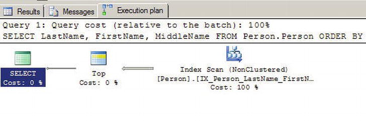
Figure 8-6. Query plan for the client-side paging implemetnation using OFFSET and FETCH
The query in Listing 8-7 is a much more readable and elegant solution for query pagination, than using the Top clause or ROW_NUMBER function with CTEs. The only exception would be if you are using OFFSET/FETCH and want to retrieve ROW_NUMBER, you would have to add ROW_NUMBER function to your query. Thus the OFFSET/FETCH clause provides a much cleaner way to implement ad-hoc pagination.
There are some restrictions though. Keep the following in mind when using OFFSET and FETCH:
- OFFSET and FETCH must be used with an ORDER BY clause.
- FETCH cannot be used without OFFSET; however OFFSET can be used without FETCH.
- Number of rows specified using OFFSET clause must be greater than or equal to 0.
- Number of rows specified by FETCH clause must be greater than or equal to 1.
- Queries that use OFFSET and FETCH cannot use the TOP operator.
- The OFFSET/FETCH values must be constants, or they must be parameters having integer values
- OFFSET and FETCH is not supported with OVER clause.
- OFFSET/FETCH is not supported with indexed views or the views WITH CHECK OPTION
In general, if operating under SQL Server 2012, the combination of OFFSET and FETCH provides for the cleanest appoarch to paginating through query results.
The RANK and DENSE_RANK Functions
The RANK and DENSE_RANK functions are SQL Server’s ranking functions. They both assign a numeric rank value to each row in a partition, however the difference lies in how ties are dealt with. For example:
- If you have three values 7, 7, and 9, then RANK wil assign ranks as 1, 1, and 3. That’s because the two 7s are tied for first place, whereas the 9 is third in the list. RANK does not respect the earlier tie when computing the rank for the value 9.
- But DENSE_RANK will assign rans 1, 1, and 2. That’s because DENSE_RANK lumps both 7s together in rank 1, and does not count them separately when computing the rank for the value 9.
There’s no right or wrong way to rank your data absent any business requirements. SQL Server provides for two options and you can choose the one that fits your business need.
Suppose you want to figure out AdventureWorks best one-day sales dates for the calendar year 2006. This scenario might be phrased with a business question like “What were the best one-day sales days in 2006?” RANK can easily give you that information, as shown in Listing 8-8. Partial results are shown in Figure 8-7.
Listing 8-8. Ranking AdventureWorks Daily Sales Totals
WITH TotalSalesBySalesDate
(
    DailySales,
    OrderDate
)
AS
(
    SELECT
        SUM(soh.SubTotal) AS DailySales,
        soh.OrderDate
    FROM  Sales.SalesOrderHeader  soh
    WHERE soh.OrderDate >= '20060101'
        AND soh.OrderDate < '20070101'
    GROUP BY soh.OrderDate
)
SELECT
    RANK() OVER
    (
        ORDER BY
        DailySales  DESC
    )  AS  Ranking,
    DailySales,
    OrderDate
FROM  TotalSalesBySalesDate
ORDER  BY  Ranking;
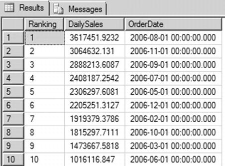
Figure 8-7. Ranking AdventureWorks daily sales totals
Listing 8-8 is a CTE that returns two columns, DailySales and OrderDate. The DailySales is the sum of all sales grouped by OrderDate. The results are limited by the WHERE clause to include only sales in the 2006 sales year.
WITH  TotalSalesBySalesDate
(
    DailySales,
    OrderDate
)
AS
(
    SELECT
        SUM(soh.SubTotal) AS DailySales,
        soh.OrderDate
    FROM  Sales.SalesOrderHeader  soh
    WHERE soh.OrderDate >= '20060101'
        AND soh.OrderDate < '20070101'
    GROUP BY soh.OrderDate
)
The RANK function is used with the OVER clause to apply ranking values to the rows returned by the CTE in descending order (highest to lowest) by the DailySales column:
SELECT
RANK() OVER ( ORDER BY
DailySales DESC ) AS Ranking, DailySales, OrderDate
FROM TotalSalesBySalesDate ORDER BY Ranking;
Like the ROW_NUMBER function, RANK can accept the PARTITION BY clause in the OVER clause. Listing 8-9 builds on the previous example and uses the PARTITION BY clause to rank the daily sales for each month. This type of query can answer a business question like “What were AdventureWorks’s best one-day sales days for each month of 2005?” Partial results are shown in Figure 8-8.
Listing 8-9. Determining the daily sales rankings partitioned by month
WITH TotalSalesBySalesDatePartitioned
(
    DailySales,
    OrderMonth,
    OrderDate
)
AS
(
    SELECT
        SUM(soh.SubTotal) AS DailySales,
        DATENAME(MONTH, soh.OrderDate) AS OrderMonth,
        soh.OrderDate
    FROM  Sales.SalesOrderHeader  soh
    WHERE soh.OrderDate >= '20050101'
        AND soh.OrderDate < '20060101'
    GROUP BY soh.OrderDate
)
SELECT
    RANK() OVER
    (
        PARTITION BY
        OrderMonth
        ORDER BY
        DailySales  DESC
    )  AS  Ranking,
    DailySales,
    OrderMonth,
    OrderDate
FROM TotalSalesBySalesDatePartitioned
ORDER BY DATEPART(mm,OrderDate),
    Ranking;

Figure 8-8. Partial results of daily sales rankings, partitioned by month
The query in Listing 8-9, like the previous example shown in Listing 8-8, begins with a CTE to calculate one-day sales totals for the year and the results are shown in Figure 8-9. The main differences between this CTE and the previous example are that Listing 8-9 returns an additional OrderMonth column and the results are limited to the year 2005. Here is that CTE:
WITH TotalSalesBySalesDatePartitioned
(
    DailySales,
    OrderMonth,
    OrderDate
)
AS
(
    SELECT
        SUM(soh.SubTotal) AS DailySales,
        DATENAME(MONTH, soh.OrderDate) AS OrderMonth,
        soh.OrderDate
    FROM  Sales.SalesOrderHeader  soh
    WHERE soh.OrderDate >= '20050101'
        AND soh.OrderDate < '20060101'
    GROUP BY soh.OrderDate
)
The SELECT query associated with the CTE uses the RANK function to assign rankings to the results. The PARTITION BY clause is used to partition the results by OrderMonth so that the rankings restart at 1 for each new month. For example:
SELECT
RANK() OVER
(
PARTITION BY OrderMonth
        ORDER BY
        DailySales  DESC
    )  AS  Ranking,
    DailySales,
    OrderMonth,
    OrderDate
FROM TotalSalesBySalesDatePartitioned
ORDER BY DATEPART(mm,OrderDate),
    Ranking;
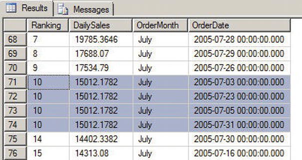
Figure 8-9. The RANK function skips a value in the case of a tie
When the RANK function encounters two equal DailySales amounts in the same partition, it assigns the same rank number to both and skips the next number in the ranking. As shown in Figure 8-9, the DailySales total for four days in July 2005 was $15012.1782, resulting in the RANK function assigning all four days a Ranking value of 10. The RANK function then skips the Ranking value from 11 through 13 and assigns the next row a Ranking of 14.
DENSE_RANK, like RANK, assigns duplicate values the same rank, but with one important difference: it does not skip the next ranking in the list. Listing 8-10 modifies Listing 8-9 to use the RANK and DENSE_RANK functions. As you can see in Figure 8-10, DENSE_RANK still assigns the same Ranking to both rows in the result, but it doesn’t skip the next Ranking value whereas RANK skips the next ranking value.
Listing 8-10. Using DENSE_RANK to Rank Best Daily Sales Per Month
WITH TotalSalesBySalesDatePartitioned
(
    DailySales,
    OrderMonth,
    OrderDate
)
AS
(
    SELECT
        SUM(soh.SubTotal) AS DailySales,
        DATENAME(MONTH, soh.OrderDate) AS OrderMonth,
        soh.OrderDate
    FROM  Sales.SalesOrderHeader  soh
    WHERE soh.OrderDate >= '20050101'
        AND soh.OrderDate < '20060101'
    GROUP BY soh.OrderDate
)
SELECT
 RANK() OVER
    (
        PARTITION BY
        OrderMonth
        ORDER BY
        DailySales  DESC
    )  AS  Ranking,
    DENSE_RANK() OVER
    (
        PARTITION BY
        OrderMonth
        ORDER BY
        DailySales  DESC
    )  AS  Dense_Ranking,
    DailySales,
    OrderMonth,
    OrderDate
FROM TotalSalesBySalesDatePartitioned
ORDER BY DATEPART(mm,OrderDate),
    Ranking;

Figure 8-10. DENSE_RANK does not skip ranking values after a tie
NTILE is another ranking function that fulfills a slightly different need. This function divides your result set into approximate n-tiles. An n-tile can be a quartile (1/4th, or 25 percent slices), a quintile (1/5th, or 20 percent slices), a percentile (1/100th, or 1 percent slices), or just about any other fractional slice you can imagine. The reason NTILE divides result sets into approximate n-tiles is that the number of rows returned might not be evenly divisible into the required number of groups. A table with 27 rows, for instance, is not evenly divisible into quar-tiles or quintiles. When you query a table with the NTILE function and the number of rows is not evenly divisible by the specified number of groups, NTILE creates groups of two different sizes. The larger groups will all be one row larger than the smaller groups, and the larger groups are numbered first. In the example of 27 rows divided into quintiles (1/5th), the first two groups will have six rows each, and the last three groups will have five rows each.
Like the ROW_NUMBER function, you can include both PARTITION BY and ORDER BY in the OVER clause. NTILE requires an additional parameter that specifies how many groups it should divide your results into.
NTILE is useful for answering business questions like “Which salespeople comprised the top 4 percent of the sales force in July 2005? and What were their sales totals?” Listing 8-11 uses NTILE to divide the AdventureWorks salespeople into four groups, each one representing 4 percent of the total sales force. The ORDER BY clause is used to specify that rows are assigned to the groups in order of their total sales. The results are shown in Figure 8-11.
Listing 8-11. Using NTILE to Group and Rank Salespeople
WITH SalesTotalBySalesPerson
(
SalesPersonID, SalesTotal
)
AS
(
SELECT
soh.SalesPersonID, SUM(soh.SubTotal) AS SalesTotal
FROM Sales.SalesOrderHeader soh
WHERE DATEPART(YEAR, soh.OrderDate) = 2005
 AND DATEPART(MONTH, soh.OrderDate) = 7
GROUP BY soh.SalesPersonID ) SELECT
NTILE(4) OVER
( ORDER BY
st.SalesTotal DESC
) AS Tile,
p.LastName,
p.FirstName,
p.MiddleName,
st.SalesPersonID,
st.SalesTotal FROM SalesTotalBySalesPerson st INNER JOIN Person.Person p
ON st.SalesPersonID = p.BusinessEntityID ;
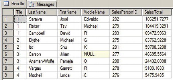
Figure 8-11. AdventureWorks salespeople grouped and ranked by NTILE
The code begins with a simple CTE that returns the SalesPersonID and sum of the order SubTotal values from the Sales.SalesOrderHeader table. The CTE limits its results to the sales that occurred for the month of July in the year 2005. Here is the CTE:
WITH SalesTotalBySalesPerson (
SalesPersonID,
SalesTotal )
AS (
SELECT
son.SalesPersonID,
SUM(soh.SubTotal) AS SalesTotal
FROM Sales.SalesOrderHeader soh
WHERE DATEPART(YEAR, soh.OrderDate) = 2005
 AND DATEPART(MONTH, soh.OrderDate) = 7
GROUP BY soh.SalesPersonID )
The SELECT query associated with this CTE uses NTILE(4) to group the AdventureWorks salespeople into four groups of approximately 4 percent each. The OVER clause specifies that the groups should be assigned based on the SalesTotal in descending order. The entire SELECT query is:
SELECT
NTILE(4) OVER
( ORDER BY
st.SalesTotal DESC
) AS Tile,
p.LastName,
p.FirstName,
p.MiddleName,
st.SalesPersonID,
st.SalesTotal FROM SalesTotalBySalesPerson st INNER JOIN Person.Person p
ON st.SalesPersonID = p.BusinessEntityID ;
Aggregate Functions, Analytic Functions, and the OVER Clause
As previously discussed, the numbering and ranking functions (ROW_NUMBER, RANK, etc.) all work with the OVER clause to define the order and partitioning of their input rows via the ORDER BY and PARTITION BY clauses. The OVER clause also provides windowing functionality to T-SQL aggregate functions such as SUM, COUNT, and SQL CLR user-defined aggregates.
Window functions help us with common business questions like those involving running totals or sliding averages. For instance, you can apply the OVER clause to the Purchasing.PurchaseOrderDetail table in the AdventureWorks database to retrieve the SUM of the dollar values of products ordered in the form of a running total. You can further restrict the resultset in which you want to perform the aggregation by partitioning the resultset by PurchaseOrderId essentially generating the running-total separately for each purchase order. An example query is shown in Listing 8-13. Partial results are shown in Figure 8-12.
Listing 8-13. Using the OVER Clause with SUM
SELECT
 PurchaseOrderID,
 ProductID,
 OrderQty,
 UnitPrice,
 LineTotal,
 SUM(LineTotal)
 OVER (PARTITION BY PurchaseOrderID
         ORDER BY ProductId
                RANGE BETWEEN UNBOUNDED PRECEDING AND CURRENT ROW)
                 AS CumulativeOrderOty
FROM Purchasing.PurchaseOrderDetail;

Figure 8-12. Partial results from query generating a running SUM
Notice the following new clause in Listing 8-13: RANGE BETWEEN UNBOUNDED PRECEDING AND CURRENT ROW
This is known as a framing clause. In this case, it specifies that each sum will include all values from the first row in the partition through to the current row. A framing clause like this makes sense only when there is order to the rows, and that is the reason for the ORDER BY ProductId clause. It is the framing clause in combination with the ORDER BY clause that together generates the running sum that you see in Figure 8-12.
![]() Tip Other framing clauses are possible. The RANGE BETWEEN UNBOUNDED PRECEDING AND CURRENT ROW in Listing 8-13 will be the default if no framing clause is specified. Keep that point in mind, as it is common for query writers to be confounded by unexpected results due to not knowing that a default framing clause is being applied.
Tip Other framing clauses are possible. The RANGE BETWEEN UNBOUNDED PRECEDING AND CURRENT ROW in Listing 8-13 will be the default if no framing clause is specified. Keep that point in mind, as it is common for query writers to be confounded by unexpected results due to not knowing that a default framing clause is being applied.
Let’s look at an example to see how the default framing clause can affect the query results. For example, let’s say you want to calculate and return the total sales amount by PurchaseOrder with each line item. Based on how the framing is defined you can get very different results since total can mean grand total or running total. Let’s modify the query in Listing 8-13 and specify the framing clause RANGE BETWEEN UNBOUNDED PRECEDING AND UNBOUNDED FOLLOWING along with the default framing clause and review the results. The modified query is shown in Listing 8-14 and results are shown in Figure 8-13.
Listing 8-14. Query results due to default framing specification
SELECT
 PurchaseOrderID,
 ProductID,
 OrderQty,
 UnitPrice,
 LineTotal,
 SUM(LineTotal)
OVER (PARTITION BY PurchaseOrderID
ORDER BY ProductId
)
AS TotalSalesDefaultFraming,
 SUM(LineTotal)
OVER (PARTITION BY PurchaseOrderID
ORDER BY ProductId RANGE BETWEEN UNBOUNDED PRECEDING
 AND UNBOUNDED FOLLOWING
)
AS TotalSalesDefinedFraming
FROM Purchasing.PurchaseOrderDetail
ORDER BY PurchaseOrderID;

Figure 8-13. Partial results from the query with different windowing specifications
In the above Figure 8-13 you can see that the Total Sales in the last 2 columns differ significantly. The column 6, TotalSalesDefaultFraming lists the total cumulative sales meaning since the framing is not specified for that column, the default framing RANGE BETWEEN UNBOUNDED PRECEDING AND CURRENT ROW is extended to this column, which means that the aggreagte is calculated only till the current row. However for column7, TotalSalesDefinedFraming the framing clause RANGE BETWEEN UNBOUNDED PRECEDING AND UNBOUNDED FOLLOWING is specified meaning the framing is extended for all the rows within the partition and hence the Total for the sales across the entire PurchaseOrder is calculated. Given the objective is to calculate and return the total sales amount for the purchase order with each line item, not specifying the framing clause yields running total. So, with the above example you can see that it is important to specify proper framing clause to achieve the desired result sets.
Now, let’s look at another example in Listing 8-15, one that modifies Listing 8-13 to return the two-day average of the total amount. In this case, we are again applying the OVER clause to the Purchasing.PurchaseOrderDetail table in the AdventureWorks database, but this time to retrieve the two-day average of the total dollr amount of products ordered. Results are sorted by by DueDate.
Notice the different framing clause in this query: ROWS BETWEEN 1 PRECEDING AND CURRENT ROW
Rows are sorted by date. For each row, the two-day average considers the current row and the row from the day previous. Partial results are shown in Figure 8-14.
Listing 8-15. Using the OVER Clause define frame sizes to return two-day, moving average
SELECT
 PurchaseOrderID,
 ProductID,
 Duedate,
 LineTotal,
 Avg(LineTotal)
 OVER (ORDER BY Duedate
 	ROWS BETWEEN 1 PRECEDING AND CURRENT ROW)
 	AS [2DayAvg]
FROM Purchasing.PurchaseOrderDetail
ORDER BY Duedate;

Figure 8-14. Partial results from a query returning a two-day, moving average
Let’s review one last scenario in which you want to calculate the running total of sales by ProductID to provide information to management on which products are selling quickly. For this example, let’s modify the query from Listing 8-15 further to define multiple windows by partitioning the resultset by ProductId. You see the resulting query in Lisitng 8-16.
You’ll be able to see how the frame expands as the calculation is done within the frame. Once the ProductId changes, the frame is reset and the calculation is restarted. Figure 8-15 shows partial result set.
Listing 8-16. Defining frames from within the OVER clause to calcualte running total
SELECT
 PurchaseOrderID,
 ProductID,
 OrderQty,
 UnitPrice,
 LineTotal,
 SUM(LineTotal) OVER (PARTITION BY ProductId ORDER BY DueDate
          RANGE BETWEEN UNBOUNDED PRECEDING AND CURRENT ROW) AS  CumulativeTotal,
 ROW_NUMBER() OVER (PARTITION BY ProductId ORDER BY DueDate ) AS  No
FROM Purchasing.PurchaseOrderDetail
ORDER BY ProductId, DueDate;

Figure 8-15. Partial results showing a running total by product ID
You can also see in the query from Listing 8-16 that you are not just limited to use one aggregate function in the SELECT statement. You can specify multiple aggregate functions in the same query.
Framing can be defined by either ROWS or RANGE with lower boundary and upper boundary. If you define only the lower boundary, then the upper boundary will be set to the current row. When you define the framing with ROWS you can specify the boundary with a number or scalar expression that returns an integer. If you do not define the boundary for framing, then the default value of RANGE BETWEEN UNBOUNDED PRECEDING AND CURRENT ROW is assumed.
Analytic Function Examples
SQL Server 2012 introduces several helpful, analytical functions. Some of the more useful of these are described in the subsections to follow. Some are statistics oriented. Others are useful for reporting scenarios in which you need to access values across rows in a result set.
CUME_DIST and PERCENT_RANK
CUME_DIST and PERCENT_RANK are two new analytical functions that have been introduced in SQL Server 2012. Suppose you want to figure out AdventureWorks Company’s best, average and worst salespeople perform in comparision to each other and especially interested in the data for the sales person Jillian Carson, whom you know exist in the table by pre-querying the data. This scenario might be phrased with a business question like “How does sales person Jillian Carson rank when compared to the total sales percentile for all the sales people?” CUME_DIST can easily give you that information, as shown in Listing 8-17. Query results are shown in Figure 8-16.
Listing 8-17. Using the CUME_DIST function
SELECT
 round(SUM(TotalDue),1) AS Sales,
 LastName,
 FirstName,
 SalesPersonId,
 CUME_DIST() OVER (ORDER BY round(SUM(TotalDue),1)) as CUME_DIST
FROM
 Sales.SalesOrderHeader soh
 	JOIN Sales.vSalesPerson sp
 	ON soh.SalesPersonID = sp.BusinessEntityID
GROUP BY SalesPersonID,LastName,FirstName;
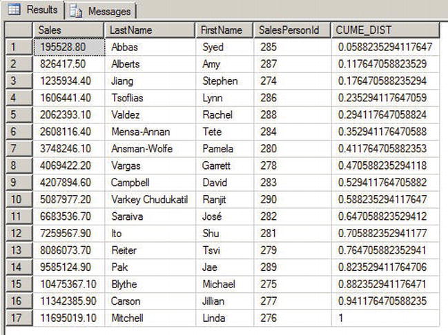
Figure 8-16. Results of CUME_DIST calculation
The query in Listing 8-17 rounds the TotalDue for the Sales Amount just to improve the query value readability. Since CUME_DIST returns the position of the row, the column results has to be formatted to return the percentage by multiplying by 100. The result in Figure 8-16 show that 94.11 % of the total salespeople have total sales less than or equal to salesperson Jillian Carson which is represented by the Cumulative distribution value of 0.9411.
If you slightly rephrase the question to “In what percentile is the total sales for sales person Jillian Carson?” PERCENT_RANK can answer that question. Listing 8-18 is a modified version Listing 8-17’s query, now including a call to PERCENT_RANK. Partial results are shown in Figure 8-17.
Listing 8-18. Using the PERCENT_RANK function
SELECT
 round(SUM(TotalDue),1) AS Sales,
 LastName,
 FirstName,
 SalesPersonId,
 CUME_DIST() OVER (ORDER BY round(SUM(TotalDue),1)) as CUME_DIST
 ,PERCENT_RANK() OVER (ORDER BY round(SUM(TotalDue),1)) as PERCENT_RANK
FROM
 Sales.SalesOrderHeader soh
 	JOIN Sales.vSalesPerson sp
 	ON soh.SalesPersonID = sp.BusinessEntityID
GROUP BY SalesPersonID,LastName,FirstName;

Figure 8-17. Results of CUME_DIST and PERCENT_RANK calculation for salesperson
The PERCENT_RANK function returns the percentage of the total sales within all the sales order in AdventureWorks. As you can see in the results, there are 17 unique values and the first value starts at 0 and the last value ends at 1 while other rows have the values based on the number of rows -1. From the above example, you can see that the salesperson Jillian Carson is at 93.75% percentile of the overall sales in AdventureWorks, which is represented by a percent rank value of 0.9375.
![]() Note You can apply the PARTITION BY clause to the CUME_DIST and PERCENT_RANK functions to define the window in which you apply those calculations.
Note You can apply the PARTITION BY clause to the CUME_DIST and PERCENT_RANK functions to define the window in which you apply those calculations.
PERCENTILE_CONT and PERCENTILE_DISC
PERCENTILE_CONT and PERCENTILE_DISC are new distribution functions that are essentially the inverse of the CUME_DIST and PERCENT_RANK functions.
Suppose you want to figure out AdventureWorks company’s 40th percentile sales total for all the accounts, it can be phrased with the business question “What is the 40th percentile for all the sales for all the accounts”. PERCENTILE_CONT and PERCENTILE_DISC requires the WITHIN GROUP clause to sepcify the ordering and the columns for the calcualtion. PERCENTILE_CONT interpolates over all the values in the window, so the result will be a calculated value whereas PERCENTILE_DISC returns the value of the actual column. Both the functions PERCENTILE_CONT and PERCENTILE_DISC requires the percentile as the argument which is a value ranges between 0.0 to 1.0. The following example in Listing 8-19 returns the answer for the business question to calcualte the sales total for the 40th percentile partitioned by account number. Hence the example uses the PERCENTILE_CONT and PERCENTILE_DISC function with the median value of 0.4 as the percentile to compute, meaning 40th percentile value. Query results are shown in Figure 8-18.
Listing 8-19. Using PERCENTILE_CONT AND PERCENTILE_DISC
SELECT
 round(SUM(TotalDue),1) AS Sales,
 LastName,
 FirstName,
 SalesPersonId,
 AccountNumber,
 PERCENTILE_CONT(0.4) WITHIN GROUP (ORDER BY round(SUM(TotalDue),1))
  OVER(PARTITION BY AccountNumber ) AS PERCENTILE_CONT,
 PERCENTILE_DISC(0.4) WITHIN GROUP(ORDER BY round(SUM(TotalDue),1))
 	OVER(PARTITION BY AccountNumber ) AS PERCENTILE_DISC
FROM
 Sales.SalesOrderHeader soh
 	JOIN Sales.vSalesPerson sp
 	ON soh.SalesPersonID = sp.BusinessEntityID
GROUP BY AccountNumber,SalesPersonID,LastName,FirstName
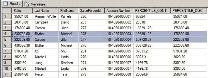
Figure 8-18. Results from the PERCENTILE_CONT AND PERCENTILE_DISC functions
You can see from the above Figure 8-18 that lists the 40th percentile for the AdventureWorks sales total and the PERCENTILE_CONT value and PERCENTILE_DISC values differ based on the account number. For account number 10-4020-000003, regardless of the salesperson, the PERCENTILE_CONT listed as 198391.28 which is an interpolated value regardless of it exists in the data set or not whereas PERCENTILE_DISC listed as 176830.40 is the value from the actual column. Whereas for the account number 10-4020-000004 the PERCENTILE_CONT listed as 308720.28 and PERCENTILE_DISC listed as 222309.60.
LAG and LEAD are new offset functions that enable you to perform calculations based on the specified row that is before or after the current row. These functions provide a method to access more than one row at a time without having to create a self join. LAG provides access to row preceding the current row, whereas LEAD provides access to the row that is after the current row.
LAG helps us answer business questions such as “For all my active products that has not been discontinued, what is the current and the previous production cost?” Listing 8-20 provides a sample query that calculates the current production cost and the last production cost for all active products using the LAG function. Partial results are shown in Figure 8-19.
Listing 8-20. Using the LAG function
WITH ProductCostHistory AS
(SELECT
ProductID,
LAG(StandardCost) OVER (PARTITION BY ProductID ORDER BY ProductID) AS PreviousProductCost,
StandardCost AS CurrentProductCost,
Startdate,Enddate
FROM  Production.ProductCostHistory
)
SELECT
ProductID,
PreviousProductCost,
CurrentProductCost,
StartDate,
EndDate
FROM ProductCostHistory
WHERE Enddate IS NULL
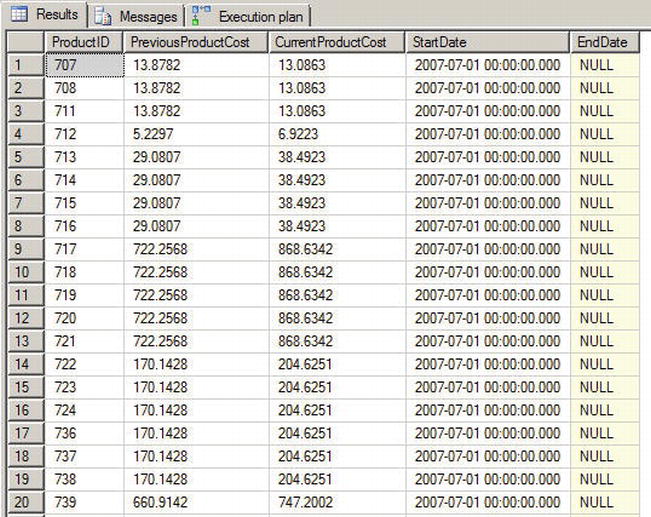
Figure 8-19. Results of production cost history comparision using the LAG fucntion
In the above example, you can see that Listing 8-20 uses the LAG function within a CTE to calculate the production cost difference between the current production cost and the previous product production cost by partitioning the data set by ProductID:
SELECT
ProductID,
LAG(StandardCost) OVER (PARTITION BY ProductID ORDER BY ProductID) AS PreviousProductCost,
StandardCost AS CurrentProductCost,
Startdate,Enddate
FROM  Production.ProductCostHistory
The SELECT query associated with the CTE returns the rows that are the latest production cost from the dataset with EndDate being null in the call:
SELECT
ProductID,
PreviousProductCost,
CurrentProductCost,
StartDate,
EndDate
FROM ProductCostHistory
WHERE Enddate IS NULL
Opposite to LAG, LEAD helps us answer business questions such as “How does each months sales compare with the sales for the following month for all the salespeople of AdventureWorks over the year 2007? ” Listing 8-21 provides a sample query that lists the next month’s total sales relative to the current month’s sales for year 2007 using the LEAD function. Partial results are shown in Figure 8-20.
Listing 8-21. Using the LEAD function
Select
 LastName,
 SalesPersonID,
 Sum(SubTotal) CurrentMonthSales,
 DateNAME(Month,OrderDate) Month,
 DateName(Year,OrderDate) Year,
 LEAD(Sum(SubTotal),1) OVER (ORDER BY SalesPersonID, OrderDate) TotalSalesNextMonth
 FROM
 Sales.SalesOrderHeader soh
 	JOIN Sales.vSalesPerson sp
 	ON soh.SalesPersonID = sp.BusinessEntityID
WHERE DateName(Year,OrderDate)  = 2007
 GROUP BY
 	FirstName, LastName, SalesPersonID,OrderDate
ORDER BY SalesPersonID,OrderDate;

Figure 8-20. Results of employee’s sales performance comparision for year 2007 using the LEAD fucntion
The above Figure 8-20 lists the results of the sales performance of the AdventureWorks sales team for year 2007. The query returns the next month’s sales total for the sales person compared to the previous months for the year 2007. You can also see that the last row returns null for the next month’s sales meaning, there is no LEAD for the last row.
FIRST_VALUE and LAST_VALUE
FIRST_VALUE and LAST_VALUE are the offset functions that return the first and last values in the window defined using the OVER clause. FIRST_VALUE returns the first value of the window, and LAST_VALUE returns the last value in the window.
These functions help us answer questions like “What are the beginning and ending sales order totals for any given month for the sales person?” Listing 8-22 provides a sample query that answers the question just posed. Partial query results are shown in Figure 8-21.
Listing 8-22. Using FIRST_VALUE and LAST_VALUE
SELECT DISTINCT
 LastName,
 SalesPersonID,
 datename(year,OrderDate) OrderYear,
 datename(month, OrderDate) OrderMonth,
 FIRST_VALUE(SubTotal) OVER (PARTITION BY SalesPersonID, OrderDate ORDER BY  SalesPersonID ) FirstSalesAmount,
 LAST_VALUE(SubTotal) OVER (PARTITION BY SalesPersonID, OrderDate ORDER BY  SalesPersonID) LastSalesAmount,
OrderDate
 FROM
 Sales.SalesOrderHeader soh
 	JOIN Sales.vSalesPerson sp
 	ON soh.SalesPersonID = sp.BusinessEntityID
ORDER BY OrderDate;

Figure 8-21. Results showing the first and last sales amount
In this example, we return the first and last sales amounts for the sales person by month and year. You can see from the Figure 8-21 that in some cases, the FirstSalesAmount and LastSalesAmount are the same, which means that there was only one sale in those months. In the months where there has been more than one sale, the amount of First Sales Order and Last Sales Order is listed.
Summary
CTEs are powerful SQL Server features that come in two varieties: recursive and nonrecursive. Nonrecursive CTEs allow you to write expressive T-SQL code that is easier to code, debug, and manage than complex queries that make extensive use of derived tables. Recursive CTEs simplify queries of hierarchical data and allow for easily generating result sets consisting of sequential numbers, which are very useful in themselves.
SQL Server’s support for windowing functions and the OVER clause makes calculating aggregates with window framing and ordering, simple. SQL Server supports several windowing functions, including the following:
- ROW_NUMBER: This function numbers the rows of a result set sequentially, beginning with 1.
- RANKandDENSE_RANK: These functions rank a result set, applying the same rank value in the case of a tie.
- NTILE: This function groups a result set into a user-specified number of groups.
- CUME_DIST, PERCENTILE_CONT, PERCENT_RANKandPERCENTILE_DISC: These functions provide analytical capabilities within T-SQL and enables cumulative distribution value calcuilations.
- LAGandLEAD: These offset functions return access to the rows at a given offset value.
- FIRST_VALUEandLAST_VALUE: These offset functions return the first and last row for a given window defined by the partition sub-clause.
You can also use the OVER clause to apply windowing functionality to built-in aggregate functions and SQL CLR user-defined aggregates.
Both CTEs and windowing functions provide useful functionality and extend the syntax of T-SQL, allowing you to write more powerful code than ever in a simpler syntax than was possible without them.
EXERCISES
- [True/false] When a CTE is not the first statement in a batch, the statement preceding it must end with a semicolon statement terminator.
- [Choose all that apply] A recursive CTE requires which of the following:
- a. The WITH keyword
- b. An anchor query
- c. The EXPRESSION keyword
- d. A recursive query
- [Fill in the blank] The MAXRECURSION option can accept a value between 0 and _________.
- [Choose one] SQL Server supports which of the following windowing functions:
- a. ROW_NUMBER
- b. RANK
- c. DENSE_RANK
- d. NTILE
- e. All of the above
- [True/false] You can use ORDER BY in the OVER clause when used with aggregate functions.
- [True/false] When PARTITION BY and ORDER BY are both used in the OVER clause, PARTITION BY must appear first.
- [Fill in the blank] The names of all columns returned by a CTE must be__________.
- [Fill in the blank] The default framing clause is ___________________.
- [True/False] If Order By is not specified for the functions that do not require in OVER clause, the window frame is defined for the entire partition
- [True/False] Checksum can be used with Over clause