Bayes theorem is the big result of Bayesian inference. Let's see how it even comes about. Recall that we previously defined the following:

That last bullet can be read as the probability that A and B occur is the probability that A occurs times the probability that B occurred, given that A already occurred.

It's from that last bullet point that Bayes theorem takes its shape.

We know that:

P(A, B) = P(A) * P(B|A)

P(B, A) = P(B) * P(A|B)

P(A, B) = P(B, A)

So:

P(B) * P(A|B) = P(A) * P(B|A)

Dividing both sides by P(B) gives us Bayes theorem, as shown:

You can think of Bayes theorem as follows:

Let's try thinking about Bayes using the terms hypothesis and data. Suppose H = your hypothesis about the given data and D = the data that you are given.

Bayes can be interpreted as trying to figure out P(H|D) (the probability that our hypothesis is correct, given the data at hand).

To use our terminology from before:

This concept is not far off from the idea of machine learning and predictive analytics. In many cases, when considering predictive analytics, we use the given data to predict an outcome. Using the current terminology, H (our hypothesis) can be considered our outcome and P(H|D) (the probability that our hypothesis is true, given our data) is another way of saying: what is the chance that my hypothesis is correct, given the data in front of me?.

Let's take a look at an example of how we can use Bayes formula at the workplace.

Consider that you have two people in charge of writing blog posts for your company—Lucy and Avinash. From past performances, you have liked 80% of Lucy's work and only 50% of Avinash's work. A new blog post comes to your desk in the morning, but the author isn't mentioned. You love the article. A+. What is the probability that it came from Avinash? Each blogger blogs at a very similar rate.

Before we freak out, let's do what any experienced mathematician (and now you) would do. Let's write out all of our information, as shown:

P(H|D) = the chance that it came from Avinash, given that you loved it

P(D|H) = the chance that you loved it, given that it came from Avinash

P(H) = the chance that an article came from Avinash

P(D) = the chance that you love an article

Note that some of these variables make almost no sense without context. P(D), the probability that you would love any given article put on your desk is a weird concept, but trust me, in the context of Bayes formula, it will be relevant very soon.

Also, note that in the last two items, they assume nothing else. P(D) does not assume the origin of the blog post; think of P(D) as if an article was plopped on your desk from some unknown source, what is the chance that you'd like it? (again, I know it sounds weird out of context).

So, we want to know P(H|D). Let's try to use Bayes theorem, as shown, here:

But do we know the numbers on the right-hand side of this equation? I claim we do! Let's see here:

When we have a suite, we can use our multiplication and addition rules, as follows:

Whew! Way to go. Now we can finish our equation, as shown:

This means that there is a 38% chance that this article comes from Avinash. What is interesting is that P(H) = .5 and P(H|D) = .38. It means that without any data, the chance that a blog post came from Avinash was a coin flip, or 50/50. Given some data (your thoughts on the article), we updated our beliefs about the hypothesis and it actually lowered the chance. This is what Bayesian thinking is all about—updating our posterior beliefs about something from a prior assumption, given some new data about the subject.

Bayes theorem shows up in a lot of applications, usually when we need to make fast decisions based on data and probability. Most recommendation engines, such as Netflix's, use some elements of Bayesian updating. And if you think through why that might be, it makes sense.

Let's suppose that in our simplistic world, Netflix only has 10 categories to choose from. Now suppose that given no data, a user's chance of liking a comedy movie out of 10 categories is 10% (just 1/10).

Okay, now suppose that the user has given a few comedy movies 5/5 stars. Now when Netflix is wondering what the chance is that the user would like another comedy, the probability that they might like a comedy, P(H|D), is going to be larger than a random guess of 10%!

Let's try some more examples of applying Bayes theorem using more data. This time, let's get a bit grittier.

Example – Titanic

A very famous dataset involves looking at the survivors of the sinking of the Titanic in 1912. We will use an application of probability in order to figure out if there were any demographic features that showed a relationship to passenger survival. Mainly, we are curious to see if we can isolate any features of our dataset that can tell us more about the types of people who were likely to survive this disaster.

First, let's read in the data, as shown here:

titanic = pd.read_csv(data/titanic.csv')#read in a csv
titanic = titanic[['Sex', 'Survived']]  #the Sex and Survived column
titanic.head()

In the preceding table, each row represents a single passenger on the ship, and, for now, we are looking at two specific features: the sex of the individual and whether or not they survived the sinking. For example, the first row represents a man who did not survive while the fourth row (with index 3, remember how python indexes lists) represents a female who did survive.

Let's start with some basics. Let's start by calculating the probability that any given person on the ship survived, regardless of their gender. To do this, let's count the number of yeses in the Survived column and divide this figure by the total number of rows, as shown here:

num_rows = float(titanic.shape[0]) # == 891 rows
p_survived = (titanic.Survived=="yes").sum() / num_rows # == .38
p_notsurvived = 1 - p_survived                          # == .61

Note that I only had to calculate P(Survived), and I used the law of conjugate probabilities to calculate P(Died) because those two events are complementary. Now, let's calculate the probability that any single passenger is male or female:

p_male = (titanic.Sex=="male").sum() / num_rows     # == .65
p_female = 1 - p_male # == .35

Now let's ask ourselves a question, did having a certain gender affect the survival rate? For this, we can estimate P(Survived|Female) or the chance that someone survived given that they were a female. For this, we need to divide the number of women who survived by the total number of women, as shown here:

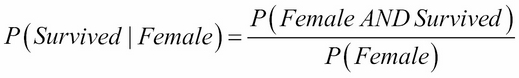
number_of_women = titanic[titanic.Sex=='female'].shape[0] # == 314
women_who_lived = titanic[(titanic.Sex=='female') & (titanic.Survived=='yes')].shape[0]                       # == 233
p_survived_given_woman = women_who_lived / float(number_of_women)
p_survived_given_woman            # == .74

That's a pretty big difference. It seems that gender plays a big part in this dataset.

Example – medical studies

A classic use of Bayes theorem is the interpretation of medical trials. Routine testing for illegal drug use is increasingly common in workplaces and schools. The companies that perform these tests maintain that the tests have a high sensitivity, which means that they are likely to produce a positive result if there are drugs in their system. They claim that these tests are also highly specific, which means that they are likely to yield a negative result if there are no drugs.

On average, let's assume that the sensitivity of common drug tests is about 60% and the specificity is about 99%. It means that if an employee is using drugs, the test has a 60% chance of being positive, while if an employee is not on drugs, the test has a 99% chance of being negative. Now, suppose these tests are applied to a workforce where the actual rate of drug use is 5%.

The real question here is of the people who test positive, how many actually use drugs?

In Bayesian terms, we want to compute the probability of drug use, given a positive test.

Let D = the event that drugs are in use

Let E = the event that the test is positive

Let N = the event that drugs are NOT in use

We are looking for P(D|E).

By using Bayes theorem , we can extrapolate it as follows:

The prior, P(D) is the probability of drug use before we see the outcome of the test, which is 5%. The likelihood, P(E|D), is the probability of a positive test assuming drug use, which is the same thing as the sensitivity of the test. The normalizing constant, P(E), is a little bit trickier.

We have to consider two things: P(E and D) as well as P(E and N). Basically, we must assume that the test is capable of being incorrect when the user is not using drugs. Check out the following equations:

So, our original equation becomes as follows:

This means that of the people who test positive for drug use, about a quarter are innocent!