
15
Parametric Spatial Audio Techniques in Teleconferencing and Remote Presence
Anastasios Alexandridis, Despoina Pavlidi, Nikolaos Stefanakis, and Athanasios Mouchtaris
Foundation for Research and Technology-Hellas, Institute of Computer Science (FORTH-ICS), Heraklion, Crete, Greece
15.1 Introduction and Motivation
In this chapter, applications of time–frequency parametric spatial audio techniques are presented in the areas of teleconferencing and remote presence. Specifically, the focus is on using circular microphone arrays in order to capture the sound field in these two different application areas. The methods presented here, consequently, have the scope to process multi-microphone signals so that the spatial properties of the original sound field can be reproduced using a multichannel loudspeaker setup or headphones as faithfully as possible, keeping as a priority computational efficiency, so that the proposed approaches can be implemented in real time using a typical PC processor.
The approaches presented are not simply extensions of established work into particular application areas, but are based on algorithms that are novel and innovative. It is relevant at this point to explain the main difference between the two application areas examined in this chapter. On the one hand, teleconference applications typically involve a small number of simultaneous sound sources at each remote participant site (the speakers at a given time instant), and the objective is to estimate their directions with respect to some reference point and reproduce the sources at these estimated directions for the receiving remote participants. On the other hand, the remote presence application area involves a more complex soundscape, where individual audio sources may not be considered as distinct, and thus estimating their direction and number is not feasible. In particular, in this chapter we focus on crowded soundscapes, such as those encountered at athletic events (for example, at a soccer game), where the objective is to reproduce the fans’ reactions for the remote participant (for example, a TV viewer). The sports event application area is an important one in terms of commercial interest, and so far has not received sufficient attention from the spatial audio community. For both application areas, real-time demonstrations of the described approaches have been developed and extensively tested in real user scenarios.1
An important aspect of the approaches presented is the focus on microphone arrays, especially of circular shape (however, the algorithms presented can easily be extended to other microphone array configurations). For the particular applications under consideration, the circular shape provides a 360° coverage around the point of interest, which can be conveniently reproduced using headphones (for example by creating a binaural signal using the corresponding head-related transfer functions – HRTFs) or via multiple loudspeakers around the listener using some amplitude panning method. A significant advantage of uniform microphone arrays made of omnidirectional microphones is the availability of several algorithms for spatial audio processing based on direction of arrival (DOA) and beamforming approaches, which often promote the use of a compact size for the microphone array, a highly desirable feature in many practical cases. At the same time, the recent introduction of digital MEMS (microelectromechanical systems) microphones (typically omnidirectional) has made feasible the design of microphone arrays that are extremely low cost, compact, and portable (since an analog to digital converter is no longer required). A picture depicting a recently built MEMS microphone array and its analog counterpart is shown in Figure 15.1.2 A digital circuit combining the MEMS microphone array with a local processor and wireless transmitter results in a microphone sensor that is an ideal device to be used in the applications under consideration in this chapter, and more generally comprises a compact and inexpensive sensor that can operate individually or as a node of a wireless acoustic sensor network (WASN).

Figure 15.1 The analog microphone array with all the necessary cables and the external multichannel sound card along with its counterpart using digital MEMS microphones. All the bulky and expensive equipment can be replaced by our digital array, which requires only one USB cable. Source: Alexandridis 2016. Reproduced with permission of the IEEE.
In the following, we initially present the state of the art in parametric spatial audio capture and reproduction, followed by a description of our approach in the two application areas of interest.
15.2 Background
In this section we briefly present the state of the art in parametric spatial audio techniques, emphasizing those methods that are based on uniform microphone arrays as the capturing device, since this is the device of interest for this chapter. The description provides the main research directions, and is by no means an exhaustive bibliographic review. See Chapter 4 for a broader introduction to the field.
Directional audio coding (DirAC; Pulkki, 2007), see also Chapter 5, represents an important paradigm in the family of parametric approaches, providing an efficient description of spatial sound in terms of one or more audio signals and parametric side information, namely the DOA and the diffuseness of the sound. While originally designed for differential microphone signals, an adaptation of DirAC to compact planar microphone arrays with omnidirectional sensors has been described by Kuech et al. (2008) and Kallinger et al. (2008), and an adaptation to spaced microphone arrangements by Politis et al. (2015). In the same direction, the approach in Thiergart et al. (2011) presents an example of how the principles of parametric spatial audio can be exploited for the case of a linear microphone array. It is also relevant to mention at this point the pioneering work of binaural cue coding (BCC; Baumgarte and Faller, 2003; Faller and Baumgarte, 2003), due to its innovative approach of encoding a spatial audio scene using one or more audio signals plus side information, which is a coding philosophy followed by several of the methods encountered in this chapter. In the context of binaural reproduction, Cobos et al. (2010) presented an approach based on a fast 3D DOA estimation technique. While not explicitly calculating any parameter related to diffuseness, the authors claimed that diffuseness information is inherently encoded by the variance in the DOA estimates. The capture and reproduction of an acoustic scene using a circular microphone array has been presented by Alexandridis et al. (2013b), and to a large extent the presented approach for the teleconference application area in this chapter is based on that work. The authors were able to show an advantage in terms of perceived spatial impression and sound quality, in a scenario with a limited number of discrete sound sources – thus suitable for applications such as teleconferencing – whose number and direction is provided by the DOA estimation and counting technique described by Pavlidi et al. (2013).
Demonstrating the applicability of parametric spatial audio techniques to large-scale sports events is certainly interesting, not only because of the great potential for commercial exploitation, but also because of the inherent technical challenges that such acoustic environments introduce. At each time instant there are hundreds of spectators cheering and applauding simultaneously from many different directions, and therefore the source sparseness and disjointness conditions that are assumed for DOA estimation are most of the time not met. Yet, techniques that attempt an accurate physical reconstruction of the sound field, such as Ambisonics (Gerzon, 1985) and wave field synthesis (Boone et al., 1995), suffer from several practical limitations. The former technique suffers from a very narrow optimal listening area, while the latter requires a prohibitively large number of loudspeakers, which is impractical for commercial use. An interesting approach that tackles these problems has been presented by Hacihabiboğlu and Cvetković (2009), using a circular array of first-order differential microphones. Essentially, the authors propose to use simple array processing in order to emulate microphones with directivity responses that conform to stereophonic panning laws. As it does not rely on any parameter estimation, this approach presents an interesting example of a non-parametric approach to sound scene capture and reproduction.
In the following sections, we present the proposed approaches for the two application areas of interest: teleconferencing, and remote presence with an emphasis on crowded acoustic environments.
15.3 Immersive Audio Communication System (ImmACS)
The Immersive Audio Communication System (ImmACS) is a spatial audio system for teleconferencing applications. ImmACS utilizes a uniform circular microphone array in order to extract spatial information from an audio scene of interest, that is, the number and the DOAs of the active audio sources. The estimates are then used for efficient encoding and transmission of the audio scene to the multiple distant participant sites.
15.3.1 Encoder
The microphone array configuration utilized in ImmACS is depicted in Figure 15.2; Figure 15.3 depicts a block diagram of the ImmACS encoder. The time-domain signals x1(t), x2(t), …, xM(t) are transformed into the short-time Fourier transform (STFT) domain signals X1(τ, ω ), X2(τ, ω), …, XM(τ, ω), where τ denotes the time frame index and ω denotes the radial frequency. The STFT domain signals are fed to the DOA estimation processing block, which returns the estimated number of active sources, ![]() , and the vector
, and the vector ![]() of DOA estimates. In parallel, the STFT signals are provided to the beamforming and post-filtering block which, given the number and DOAs of the sources, produces
of DOA estimates. In parallel, the STFT signals are provided to the beamforming and post-filtering block which, given the number and DOAs of the sources, produces ![]() separated signals
separated signals ![]() . The separated signals are efficiently downmixed into a single audio channel, e(t), and side information I(τ, ω).
. The separated signals are efficiently downmixed into a single audio channel, e(t), and side information I(τ, ω).

Figure 15.2 Uniform circular microphone array configuration. The microphones are numbered 1 to M and the sound sources are s1 to sP.The array radius is denoted as q, α and l are the angle and distance between adjacent microphones, and A is the obtuse angle formed by the chord defined by microphones 1 and 2 and the x-axis; θ1 indicates the DOA of source s1. Adapted from Pavlidi 2013.

Figure 15.3 Block diagram of ImmACS encoder. Source: Alexandridis 2013a. https://www.hindawi.com/ journals/jece/2013/718574/. Used under CC BY 3.0.
Counting and DOA Estimation of Multiple Audio Sources
For the counting and estimation of the DOAs, ImmACS adopts a relaxed sparsity assumption on the time–frequency (TF) domain of the source signals (Puigt and Deville, 2007; Pavlidi et al., 2012). It is assumed that for each source at least one constant-time analysis zone can be found where the source is isolated, that is, it is dominant over the others. The constant-time analysis zone is defined as a series of Ω frequency-adjacent TF points at time frame index τ, denoted by (τ, Ω), and it is characterized as a single-source zone (SSZ) if it is dominated by one audio source. Such a sparsity assumption allows the signals to overlap in the time–frequency domain. It is therefore a much weaker constraint compared to the W-disjoint orthogonality assumption (Rickard and Yilmaz, 2002), where every TF point is considered to be dominated by one source. In ImmACS, DOA estimation of multiple sources relies on the detection of all SSZs and the derivation of local DOA estimates, deploying a single-source localization algorithm.
To detect an SSZ, the cross- and auto-correlation of the magnitude of the TF transform need to be estimated (in what follows, the time frame index, τ, is dropped for clarity):
The correlation coefficient between a pair of microphone signals (xi, xj) is then defined as

A constant-time analysis zone is an SSZ if and only if (Puigt and Deville, 2007)
In practice, every zone that satisfies the inequality
is characterized as an SSZ, where ![]() is the average correlation coefficient between pairs of observations of adjacent microphones and ε is a small user-defined threshold.
is the average correlation coefficient between pairs of observations of adjacent microphones and ε is a small user-defined threshold.
The SSZ detection stage is followed by the DOA estimation at each SSZ. In general, any suitable single-source DOA estimation algorithm could be applied. In ImmACS, a modified version of the algorithm in Karbasi and Sugiyama (2007) is deployed, mainly because this algorithm is designed specifically for circular apertures, is computationally efficient, and has shown good performance under noisy conditions (Karbasi and Sugiyama, 2007; Pavlidi et al., 2013).
The phase of the cross-power spectrum of a microphone pair is first evaluated over the frequency range of an SSZ as

where the cross-power spectrum is
and * stands for complex conjugate.
The evaluated cross-power spectrum phase is used to estimate the phase rotation factors (Karbasi and Sugiyama, 2007),
where τi → 1(ϕ)≜τ1, 2(ϕ) − τi, i + 1(ϕ) is the difference in the relative delay between the signals received at pairs {1, 2} and {i, i + 1}. The time difference of arrival for the microphone pair {i, i + 1} is evaluated according to
where ϕ ∈ [0, 2π), ω ∈ Ω, α and l are the angle and distance between the adjacent microphone pair {i, i + 1} respectively, A is the obtuse angle formed by the chord defined by the microphone pair {1, 2} and the x-axis, and c is the speed of sound (see also Figure 15.2). Since the microphone array is uniform, α, A, and l are given by
where q is the array radius.
Next comes the estimation of the circular integrated cross spectrum (CICS), defined by Karbasi and Sugiyama (2007) as

The DOA associated with the frequency component ω in the SSZ with frequency range Ω is estimated as
In order to enhance the overall DOA estimation, the aforementioned algorithm is applied on “strong” frequency components, that is, those frequencies that correspond to the indices of the d highest peaks in the magnitude of the cross-power spectrum over all microphone pairs in an SSZ. Figure 15.4 illustrates the DOA estimation error versus signal to noise ratio (SNR) for various choices of d. It is clear that using more frequency bins leads in general to a lower estimation error. However, increasing d increases the computational complexity, which has to be taken into consideration for a real-time system. In ImmACS, a standard choice for d is d = 2.

Figure 15.4 Direction of arrival estimation error vs. SNR in a simulated environment. Each curve corresponds to a different number of frequency components used in a single-source zone. Source: Pavlidi 2013. Reproduced with permission of the IEEE.
The next step in counting and estimating the final DOAs of active audio sources constitutes the processing of estimated DOAs in SSZs in a block-based manner. To do so, a histogram is formed from the set of estimations in a block of B consecutive time frames, which slides one frame each time. The histogram is smoothed by applying an averaging filter with a window of length hN, providing

where y(v) is the cardinality of the smoothed histogram at each histogram bin v, V is the number of bins in the histogram, ζi is the ith estimate out of N estimates in a block, and w( · ) is the rectangular window of length hN.
The smoothed histogram is processed following the principles of matching pursuit, that is, it is correlated with a source atom in order to detect the DOA of a possible source, the contribution of which is estimated and removed from the histogram. The process is repeated iteratively until the contribution of a potential source fails to satisfy a user-defined threshold.
A narrower-width pulse is used to accurately locate a peak in the histogram, the index of which denotes the DOA of a source. A wider-width pulse is used to account for the contribution of the source to the overall histogram and to provide better performance at lower SNRs. Each source atom is modeled as a smooth pulse utilizing a Blackman window. The correlation of the histogram with the source atom is performed in a circular manner as the histogram “wraps” from 359° to 0°. Thus, a matrix has to be formed whose rows contain wrapped and shifted versions of the source pulse. We denote by CN and CW the matrices for the peak detection (denoted by “N” for narrow) and the contribution estimation (denoted by “W” for wide), respectively. The rows of matrix CN contain shifted versions of the narrow source atom with width QN, and, correspondingly, the rows of matrix CW contain the shifted wide source atom with width equal to QW. This dual-width approach is illustrated in Figure 15.5.

Figure 15.5 A wide source atom (dashed line) and a narrow source atom (solid line) applied to the smoothed histogram of four sources (speakers). Source: Pavlidi 2013. Reproduced with permission of the IEEE.
In more detail, at each iteration denoted with loop index j, u = CNyj is formed, where yj is the smoothed histogram at the current iteration. u denotes the correlation of the histogram with the narrow pulse, and thus the index of its maximum value denotes the DOA estimated at the current iteration j, that is, ![]() , where ui are the elements of u. The contribution of the source located at iteration j is estimated as
, where ui are the elements of u. The contribution of the source located at iteration j is estimated as

Observe that the contribution is actually the row of the matrix CW that contains a circularly shifted version of the source atom by (i* − 1) elements, that is, c(i* − 1)W, weighted by ![]() . In order to decide if the detected DOA and its contribution correspond to a true source and ultimately estimate the number of active sources,
. In order to decide if the detected DOA and its contribution correspond to a true source and ultimately estimate the number of active sources, ![]() , we create
, we create ![]() , a length-PMAX vector whose elements are some predetermined thresholds, representing the relative energy of the jth source. Thus, if
, a length-PMAX vector whose elements are some predetermined thresholds, representing the relative energy of the jth source. Thus, if ![]() then a source is detected and its contribution is removed from the histogram:
then a source is detected and its contribution is removed from the histogram:
The algorithm then proceeds with the next iteration. In the opposite case, the algorithm ceases and the estimated DOAs and their corresponding number are returned.
Beamforming and Downmixing
Based on the estimated number of sources and their corresponding DOAs, ImmACS utilizes a spatial filter that consists of a superdirective beamformer and a post-filter in order to separate the sources’ signals. The superdirective beamformer is designed to maximize the array gain, keeping the signal from the steering direction undistorted, while maintaining a minimum constraint on the white noise gain; the beamformer’s filter coefficients are given by (Cox et al., 1987)
where w(ω, θ) is the M × 1 vector of complex filter coefficients, θ is the beamformer’s steering direction, d(ω, θ) is the steering vector of the array, ![]() is the M × M noise coherence matrix, ( · )H is the Hermitian transpose operation, I is the identity matrix, and ε is used to control the white noise gain constraint. Assuming a spherically isotropic diffuse noise field, the elements for the noise coherence matrix are calculated as
is the M × M noise coherence matrix, ( · )H is the Hermitian transpose operation, I is the identity matrix, and ε is used to control the white noise gain constraint. Assuming a spherically isotropic diffuse noise field, the elements for the noise coherence matrix are calculated as

where ω denotes the radial frequency, c is the speed of sound, and dij is the distance between the ith and jth microphones. The beamformer is signal independent, facilitating its use in the real-time implementation of ImmACS, as the filter coefficients are calculated offline and stored in the system’s memory.
Hence, for each source s, the microphone signals at frequency ω are filtered with the beamformer filter coefficients w(ω, θs) that correspond to the source’s estimated direction θs. This procedure results in the beamformer output signals:
A post-filtering operation is then applied to the beamformer output signals; each beamformer output signal is filtered with a binary mask. The binary masks are constructed by comparing the energies of the beamformer output signals for each source at a given frequency. The binary mask for the sth source is given by (Maganti et al., 2007)
The final separated source signals are given by:
From Equation (15.18), it is obvious that the binary masks are orthogonal with respect to each other. This means that if Us(τ, ω) = 1 for some frequency ω and frame index τ, then ![]() for s′ ≠ s, a property which also holds for the final separated source signals. This means that for each frequency only one source is maintained – the one with the highest energy – while the other sources are set to zero. The effect of the post-filtering operation is illustrated with an example of three active sound sources in Figure 15.6: for each frequency, only the source with the highest energy is kept, for example the first source for frequency ω1, the third source for frequency ω2, and so on. Looking at the frequency domain representation of the resulting post-filtered signals in Figure 15.6(b), the orthogonality property of the binary masks is evident.
for s′ ≠ s, a property which also holds for the final separated source signals. This means that for each frequency only one source is maintained – the one with the highest energy – while the other sources are set to zero. The effect of the post-filtering operation is illustrated with an example of three active sound sources in Figure 15.6: for each frequency, only the source with the highest energy is kept, for example the first source for frequency ω1, the third source for frequency ω2, and so on. Looking at the frequency domain representation of the resulting post-filtered signals in Figure 15.6(b), the orthogonality property of the binary masks is evident.

Figure 15.6 Examples of: (a) beamformer output signals, and (b) post-filtered signals, for a scenario of three active sound sources.
The orthogonality property of the binary masks results in a very efficient downmixing scheme: the sources’ signals can be downmixed by summing them in the frequency domain to create a full-spectrum monophonic audio signal:

The downmix signal is then transformed back to the time-domain signal e(t). To extract the estimated source signals from the downmix, additional information must also be attained, describing to which source each frequency of the downmix belongs. For this reason, ImmACS creates a side-information channel I(τ, ω), which attains the assignment of frequencies to the DOAs of the sources, which also specifies the direction from which each frequency of the downmix signal will be reproduced in the decoder. Hence, the entire soundscape is encoded with the use of one monophonic audio signal and side information. These two streams are transmitted to the decoder in order to recreate and reproduce the soundscape.
ImmACS also offers the potential to include a diffuse part in the encoded soundscape. This is done by setting a cut-off frequency ωc, which defines the frequencies up to which directional information is extracted: for the frequencies below ωc, the aforementioned procedure of spatial filtering is applied in order to separate the active sources’ signals. In contrast, the frequencies above ωc are assumed to be dominated by diffuse sound. For these frequencies the spectrum from an arbitrary microphone of the array is included in the downmix (the dashed line in Figure 15.3), without further processing and without the need to keep any side information for this part, as it represents the part of the soundscape with no prominent direction. Thus, the side-information channel only attains the directional information for the frequencies up to ωc. Processing only a certain range of frequencies may have several advantages, such as reduction in the computational complexity – especially when the sampling frequency is high – and reduction in the bitrate requirements for the side-information channel. But, more importantly, treating the higher frequencies as diffuse sound offers a sense of immersion to the listeners. Finally, applications like teleconferencing, where the signal content is mostly speech, can tolerate setting ωc to approximately 4 kHz without degradation in the spatial impression of the recreated soundscape.
To reduce the bitrate requirements, coding schemes can be applied to both the audio and the side-information channels. Since the audio channel consists of a monophonic stream, any monophonic audio encoder can be utilized, such as MP3 (ISO, 1992), or the ultra-low-delay OPUS coder (Valin et al., 2013; Vos et al., 2013) that is used in ImmACS. Encoding the downmix signal with any of the aforementioned codecs has been found not to affect the spatial impression of the recreated soundscape (Alexandridis et al., 2013b).
To encode the side-information channel, lossless coding schemes need to be used in order to attain the assignment of the frequencies to the sources. The side-information channel depends on Equation (15.18), and thus it is sufficient to encode the binary masks. The encoding scheme that ImmACS employs is based on the orthogonality property of the masks, as explained below.
The active sources at a given time frame are sorted in descending order according to the number of frequency bins assigned to them. The binary mask of the first (the most dominant) source is inserted into the bitstream. Given the orthogonality property of the binary masks, it follows that we do not need to encode the mask for the sth source at the frequency bins where at least one of the previous s − 1 masks is equal to one (since the rest of the masks will be zero). These locations can be identified by a simple OR operation between the s − 1 previous masks. Thus, for the second up to the ![]() th mask, only the locations where the previous masks are all zero are inserted into the bitstream. The mask of the last source does not need to be encoded, as it contains ones in the frequency bins in which all the previous masks had zeros. A dictionary that associates the sources with their DOAs is also included in the bitstream. The encoding algorithm is presented in Algorithm 15.1 and is illustrated with an example in Figure 15.7. In Algorithm 15.1, find_positions_with_zeros(·) is a function that returns the indices of zero values of the vector taken as argument, and | denotes the concatenation operator. The resulted bitstream is further compressed with Golomb entropy coding (Golomb, 1966) applied on the run lengths of ones and zeros.
th mask, only the locations where the previous masks are all zero are inserted into the bitstream. The mask of the last source does not need to be encoded, as it contains ones in the frequency bins in which all the previous masks had zeros. A dictionary that associates the sources with their DOAs is also included in the bitstream. The encoding algorithm is presented in Algorithm 15.1 and is illustrated with an example in Figure 15.7. In Algorithm 15.1, find_positions_with_zeros(·) is a function that returns the indices of zero values of the vector taken as argument, and | denotes the concatenation operator. The resulted bitstream is further compressed with Golomb entropy coding (Golomb, 1966) applied on the run lengths of ones and zeros.


Figure 15.7 Example of the side-information coding scheme for a scenario of four active sound sources. All frequencies of the mask of the first source (the most dominant) are stored. For the second mask, only the frequencies where the first mask is zero need to be stored, as the other frequencies will definitely have the value of zero in the second and all other masks (orthogonality property). For each next mask, only the frequencies where all previous masks are zero need to be stored. Source: Alexandridis 2013. Reproduced with permission of the University of Crete.
15.3.2 Decoder
The decoder recreates the soundscape for the remote participants according to the block diagram depicted in Figure 15.8. Based on the available equipment, ImmACS supports multichannel reproduction using multiple loudspeakers, Figure 15.8(a), or binaural reproduction using headphones, Figure 15.8(b).
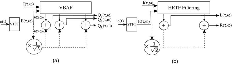
Figure 15.8 Block diagram of ImmACS decoder for (a) loudspeaker reproduction and (b) binaural reproduction. Source: Alexandridis 2013a. https://www.hindawi.com/journals/jece/2013/718574/. Used under CC BY 3.0.
In the case where the downmix signal or the side-information channel have been encoded, the respective decoder is first applied. For decoding the side information, the mask of the first source is retrieved first. For the mask of the sth source, the next n bits are read from the bitstream, where n is the number of frequencies for which all the previous s − 1 masks are zero. This can be identified by a simple NOR operation. In terms of complexity, this scheme is computationally efficient, as its main operations are simple OR and NOR operations.
Then, for every incoming frame, the downmix signal e(t) is transformed to the frequency domain and the spectrum is divided into the non-diffuse part and diffuse part, based on the beamformer cutoff frequency ωc: the frequencies ω ≤ ωc belong to the non-diffuse part, while the diffuse part—if it exists—includes the frequencies ω > ωc.
For loudspeaker reproduction, the non-diffuse part is synthesized using vector base amplitude panning (VBAP; Pulkki, 1997) at each frequency, where the panning gains for each loudspeaker are determined according to the DOA at that frequency from the side-information channel I(τ, ω). If a diffuse part is included, it is played back from all loudspeakers (dashed line in Figure 15.8(a)). Assuming a loudspeaker configuration with L loudspeakers, the signal for the lth loudspeaker is thus given by

where gl(I(τ, ω)) refers to the VBAP gain for the lth loudspeaker in order to play back the time–frequency point (τ, ω) from the direction specified by I(τ, ω).
For binaural reproduction using headphones, ImmACS utilizes an HRTF database in order to position each source at its corresponding direction. Hence, each frequency of the non-diffuse part is filtered with the HRTF of the direction specified by the side information. The optional diffuse part is included in both channels – the dashed line in Figure 15.8(b). Summarizing, the two-channel output is given by

where ![]() denotes the left and right channels.
denotes the left and right channels.
15.4 Capture and Reproduction of Crowded Acoustic Environments
Typically, capturing large sports events is accomplished with several microphones placed around the pitch or inside the crowd, so that each microphone focuses on a particular segment of the event (Cengarle et al., 2010). A great amount of equipment needs to be carefully distributed all around the playing field, requiring a lot of preparation time and attendance during the game. Then, it depends on the experience and subjective judgment of the sound engineer to mix all the signals into the final stereo or surround format that is transmitted by the broadcaster. The approach of using one or just a few compact sensor arrays to capture and reproduce sound from such large-scale events presents an interesting alternative; it may reduce the cost of equipment and implementation, allow flexibility in the processing and manipulation of the captured spatial information (Stefanakis and Mouchtaris, 2015, 2016), and allow for efficient encoding of the data to reduce bandwidth requirements during transmission (Alexandridis et al., 2013a).
In this section we present two different approaches, a parametric and a non-parametric one, for the capture and reproduction of a sound scene in 2D using a circular sensor array of omnidirectional microphones. Such a study is interesting as it further extends the range of applications in which circular microphone arrays find a use, but also because it puts two inherently different approaches to the test. The techniques presented are applied to a real recording, produced inside a crowded football stadium with thousands of spectators.
15.4.1 Sound Source Positioning Based on VBAP
Sound source positioning using VBAP (Pulkki, 1997) is traditionally linked to virtual sound source placement and to parametric spatial audio applications, where a DOA θ with respect to some portion of the signal is always defined or estimated. VBAP requires that the loudspeakers are distributed around a circle of fixed radius around the listening area, but their number and direction might be arbitrary, a fact that provides important flexibility in designing the loudspeaker arrangement. Given the incident angle θ, this is mapped to the L loudspeaker gains ![]() in accordance with the physical loudspeaker distribution around the listening area. In Figure 15.9 we show an example of how such directivity patterns look for the cases of L = 4 and 8 uniformly distributed loudspeakers in Figure 15.9(a) and Figure 15.9(c), and for L = 5 non-uniform loudspeakers in Figure 15.9(b), assuming that the problem is confined to 2D.
in accordance with the physical loudspeaker distribution around the listening area. In Figure 15.9 we show an example of how such directivity patterns look for the cases of L = 4 and 8 uniformly distributed loudspeakers in Figure 15.9(a) and Figure 15.9(c), and for L = 5 non-uniform loudspeakers in Figure 15.9(b), assuming that the problem is confined to 2D.

Figure 15.9 Desired directivity patterns for (a) a four-channel, (b) a five-channel and (c) an eight-channel system. Source: Stefanakis and Mouchtaris 2016.
It is worth spending a few words here in order to explain how the aforementioned mapping between incident angle and loudspeaker gain is also useful in the case of the non-parametric approach which we intend to consider. Hacihabiboğlu and Cvetković (2009) explain how the physical loudspeaker angular distribution dictates the optimum directivity patterns for an equal (to the number of loudspeakers) number of directional microphones to capture the directional properties of the sound field. Given such microphones, one could then send the signal captured by each microphone to the corresponding loudspeaker, without further processing, to reproduce a convincing panoramic auditory reality. Respecting the requirements stated in that paper, VBAP dictates optimal loudspeaker panning gains with the following characteristics:
- the panning gains are frequency-invariant;
- the problem of unwanted interchannel crosstalk is efficiently addressed by ensuring that given a single plane wave incident at a certain angle (in the azimuth plane), only two loudspeakers will be activated during reproduction (the two that are adjacent to the estimated angle);
- the sum of the squares of all loudspeaker gains along θ is equal, meaning that there is no information loss.
This implies that we can use the loudspeaker gains provided by VBAP as the desired directivity response for a set of beamformers, which we can then use in order to capture the acoustic environment in different directions. The signal at the output of each beamformer can then be sent directly to the corresponding loudspeaker, a process that is mathematically represented in Equation (15.23). As long as the desired beam patterns are accurately reproduced, the non-parametric approach represents the simplest way to capture and reproduce an acoustic scene, promising accurate spatialization of both the directional and diffuse components of the captured sound field. As will be seen, however, the accurate reconstruction of these patterns using beamforming is not an easy task, and deviations between the desired and actually reproduced directivity patterns are expected to degrade the sense of direction transmitted to the listener.
15.4.2 Non-Parametric Approach
In the time–frequency domain, the process of beamforming can be expressed as
where τ is the time-frame index, ω is the radial frequency, wl(ω) = [w1l(ω), …, wMl(ω)]T is the vector with the M complex beamformer weights responsible for the lth loudspeaker channel, X(τ, ω) is the M × 1 vector with the signal at the microphones, and Yl(τ, ω) represents the lth loudspeaker signal in the time–frequency domain. This process is repeated for all the different loudspeaker channels l = 1, …, L; the signals are transformed to the time domain and sent to the corresponding loudspeakers for playback.
Using the panning gains dictated by VBAP, we demonstrate in what follows an approach for calculating the beamformer weights associated with each loudspeaker channel. Consider a grid of N uniformly distributed directions θn in [ − 180°, 180°) with the loudspeaker panning gains gl(θn) prescribed by VBAP. The problem becomes finding the weights wl(ω) in order to satisfy
Here, Gl = [gl(θ1), …, gl(θN)]T is the desired response provided by VBAP and D(ω) = [d(ω, θ1), …, d(ω, θN)] is the matrix with the array steering vectors which model the array response to a plane wave incident at angle θn. Without loss of generality we may consider here that ![]() ∀l as the VBAP function does not dictate phase variations across the different channels. Also, for the case of a circular array of radius R the propagation model can be written as (Alexandridis et al., 2013a)
∀l as the VBAP function does not dictate phase variations across the different channels. Also, for the case of a circular array of radius R the propagation model can be written as (Alexandridis et al., 2013a)
where ϕm denotes the angle of the mth sensor with respect to the sensor array center and k is the wavenumber. Assuming that L < N, the linear problem of Equation (15.24) is overdetermined and the solution can be found by minimizing, in the least squares (LSQ) sense, the cost function
However, unconstrained minimization involves inversion of the matrix D(ω)D(ω)H, which is ill-conditioned at low frequencies as well as at other distinct frequencies. An example of this behavior is shown in Figure 15.10, where we have plotted the condition number of D(ω)D(ω)H as a function of frequency, considering a circular array of M = 8 uniformly distributed microphones and the reproduction system of Figure 15.9(a). Direct inversion of D(ω)D(ω)H might thus lead to severe amplification of noise at certain frequencies, which is perceived as unwanted spectral coloration. In order to avoid such a problem, we propose to use Tikhonov regularization by adding a penalty term proportional to the noise response in the previous cost function as
with μ(ω) implying that the value of the regularization parameter varies with frequency. We have observed that this approach achieves a better trade-off between the noise gain and the array gain, as opposed to a constant value of the regularization parameter. In this chapter, we propose a varying value of the regularization parameter of the form
where λ is a fixed scalar and cond(·) represents the condition number of a matrix, that is, the ratio of its largest eigenvalue to its smallest one. The beamformer weights can then be found through LSQ minimization as
where I is the M × M identity matrix.

Figure 15.10 Condition number of matrix D(ω)HD(ω) in dB (black) and variation of the regularization parameter μ (gray) as a function of the frequency for an eight-sensor circular array of radius 5 cm. Source: Stefanakis and Mouchtaris 2016.
Finally, we consider an additional normalization step, which aims to ensure unit gain and zero phase shift at the direction of maximum response for each beamformer. Letting θ0l denote this direction for the lth beam at frequency ω, the final weights are calculated as

and the signal for the lth loudspeaker is obtained as in Equation (15.23). The beamformer weights need only be calculated once for each frequency and then stored to be used in the application phase.
In Figure 15.11 we present plots of the actual directivity versus the desired directivity pattern, for the same reproduction system as considered in Figure 15.9. Observe the increment in the amplitude of the side-lobes at 2660 Hz, which is close to a problematic frequency according to Figure 15.10. Also, the subplot corresponding to 7 kHz (in Figure 15.11) is indicative of the spatial aliasing problems that occur at higher frequencies.

Figure 15.11 Actual directivity patterns (solid black) versus desired directivity patterns (dashed gray) at different frequencies for an eight-element circular sensor array. The directivity patterns shown correspond to the first loudspeaker at 45°, considering a symmetric arrangement of four loudspeakers at angles of 45°, 135°, −135°, and −45° degrees. Source: Stefanakis and Mouchtaris 2016.
15.4.3 Parametric Approach
As shown in Figure 15.11, it is difficult to obtain exactly the desired directivity patterns relying on simple beamforming. Looking, for example, at the sub-figure corresponding to 2660 Hz, we see that a sound source at −135° would also be played back by the loudspeaker at 45°, something that may blur the sense of direction transmitted to the listener. On the other hand, a parametric approach avoids this problem by defining the loudspeaker response as a function of the estimated DOA.
However, it is questionable what type of processing is applicable to the particular type of array that we typically focus on in our work. While the method works sufficiently well for an application with a limited number of speakers, such as the one described in Section 15.3, it is inappropriate for the considered acoustic conditions due to the enormous number of potential sound sources that participate in the sound scene. On the other hand, DirAC does not impose a limitation on the number of sound sources comprising the sound scene, but it is typically implemented with smaller arrays – in terms of both radius and number of sensors – than the one considered in this application (Kuech et al., 2008).
The parametric approach that we present in this section is based on the method introduced by Ito et al. (2010). We exploit this previous study here in order to perform direct-to-diffuse sound field decomposition, at the same time extending it for the purpose of DOA estimation. Assume that a sensor array comprised of M sensors is embedded inside a diffuse noise field and at the same time receives the signal from a single directional source. The observation model for sensor m can be written
where s(τ, ω) is the directional source signal, ![]() is the transfer function from the source to the sensor at frequency ω, and Um(τ, ω) is the diffuse noise component, which is assumed to be uncorrelated with the source signal. The observation interchannel cross-spectrum between sensors m and n can thus be written
is the transfer function from the source to the sensor at frequency ω, and Um(τ, ω) is the diffuse noise component, which is assumed to be uncorrelated with the source signal. The observation interchannel cross-spectrum between sensors m and n can thus be written
where ϕss is the source power spectrum and ![]() represents the component of the cross-spectrum due to noise. Assuming that the noise field is isotropic, then
represents the component of the cross-spectrum due to noise. Assuming that the noise field is isotropic, then ![]() , as explained in Ito et al. (2010). This means that the imaginary part of the cross-spectra observation is immune to noise, and therefore depends only on the directional source location. According to this, one may write
, as explained in Ito et al. (2010). This means that the imaginary part of the cross-spectra observation is immune to noise, and therefore depends only on the directional source location. According to this, one may write
where ℑ{ · } denotes the imaginary part of a complex number. We may now use this observation in order to create a model of the imaginary cross-spectra terms through the vector
which contains all the M(M − 1)/2 pairwise sensor combinations, with delays δm(θ) and δn(θ) defined according to the incident plane wave angle θ. This vector can be seen as an alternative steering vector with the property a(ω, θ ± π) = −a(ω, θ), for θ in radians. Consider now the vector constructed by the vertical concatenation of M(M − 1)/2 imaginary observation cross-spectra terms as
where Φmn(τ, ω) corresponds to the element at the mth row and nth column of the signal covariance matrix
Now, z(τ, ω) in Equation (15.36) represents an immune-to-noise observation of the sound field, which should be consistent with respect to the model in Equation (15.35), given that the sound field is a plane wave with an incident angle θ. The most likely DOA at frequency ω and time frame τ can be found by searching for the plane wave signature a(ω, θ) that is most similar to z(τ, ω):
where ![]() implies normalization with the Euclidean norm so that all plane wave signatures have the same energy. The source power spectrum at the particular TF point is then found by projecting a(ω, θτ, ω) onto z(τ, ω) as
implies normalization with the Euclidean norm so that all plane wave signatures have the same energy. The source power spectrum at the particular TF point is then found by projecting a(ω, θτ, ω) onto z(τ, ω) as

On the other hand, an estimation of the total acoustic power can be found by averaging the power across all microphones as ϕyy(τ, ω) = tr(Φ)/M, where tr( · ) is the sum of all the diagonal terms of a matrix. The ratio q(τ, ω) = ϕss(τ, ω)/ϕyy(τ, ω) then represents a useful metric that can be associated with the diffuseness of the sound field; intuitively, 0 ≤ q(τ, ω) ≤ 1 should hold, with a value close to 1 dictating a purely directional sound field whereas a value close to 0 implies a purely noisy sound field. Furthermore, we may use this metric in order to establish a relation with the so-called diffuseness of the sound field:
where the function min{ · } returns the minimum of a set of numbers and is useful here in order to ensure that the diffuseness does not take negative values, if q(τ, ω) > 1.
The input signal at the lth loudspeaker is then synthesized as Yl(τ, ω) = Ydirl(τ, ω) + Yτ, difl(ω), where
Here, Xref(τ, ω) is the captured signal at a reference microphone (the first microphone), gl is the VBAP gain responsible for the lth loudspeaker and ![]() are the beamformer weights derived in Section 15.4.3. As can be seen, at each TF point, the diffuse channels of this method are nothing but a weighted replica of the loudspeakers signals produced with the parametric technique of Section 15.4.2.
are the beamformer weights derived in Section 15.4.3. As can be seen, at each TF point, the diffuse channels of this method are nothing but a weighted replica of the loudspeakers signals produced with the parametric technique of Section 15.4.2.
15.4.4 Example Application
Both the parametric and the non-parametric approaches presented above were applied to a real recording produced with the eight-microphone circular array of radius R = 0.05 m shown in Figure 15.12(a). The recording took place in a crowded open stadium during a football match of the Greek Super League. Figure 15.12(b) presents a sketch of the football stadium with the location of the array represented by a white dot. The array was placed at a height of 0.8 m in front of Gates 13 and 14, which were populated with the organized fans of the team which was hosting the game. These fans were cheering and singing constantly throughout the entire duration of the recording, thus providing most of the acoustic information captured by the array.

Figure 15.12 (a) The sensor array. (b) Sketch of the football stadium with the loudspeaker setup used for evaluation. The white dot in the lower-right corner of the football field denotes the array location. Source: Stefanakis and Mouchtaris 2016.
The reproduction system that we considered for the application phase consisted of four loudspeakers uniformly distributed around the azimuth plane, specifically at 45°, 135°, −135°, and −45° (see Figure 15.12), at a radius of 2.10 m. With respect to the listener’s orientation, these loudspeakers were located at rear right (RR), front right (FR), front left (FL), and rear left (RL). This configuration is of particular interest as it can easily be extended with a 5.1 surround system, adding one more channel to be used for the commentator. The panning gains derived from VBAP for this setup are identical to those depicted in Figure 15.9(a).
The signals were recorded at 44 100 Hz and processed separately with the parametric and the non-parametric approach. For the STFT we used a Hanning window of length 2048 samples and hop size 1024 samples (50% overlap). For the non-parametric method, we used the frequency-varying regularization parameter of Equation (15.28), with λ = 0.003. The variation of μ as a function of the frequency is illustrated with the gray line in Figure 15.10, while the polar plots of Figure 15.11 are illustrative of the deviation between the desired and the actual beamformer directivities.
Avoiding the problem with the imperfect beam shapes of the non-parametric method, one expects the parametric approach to produce better localization of the different acoustic sources. The opinion of the authors, who were also present inside the stadium during the recording, is that the parametric method indeed produced a more convincing sense of direction in comparison to beamforming, and was also more consistent with respect to changes in the orientation of the listener’s head inside the listening area, as well as with reasonable displacements from the sweet spot. On the other hand, the non-parametric method provided a more blurred sense of direction but a much better sense of the reverberation in the stadium. As additional evidence for this contradiction between the two methods, we have plotted in Figure 15.13 the rectified loudspeakers’ signal amplitudes in time, as derived by each technique, for a short-duration segment where the crowd at Gates 13 and 14 was by far the most dominant acoustic source inside the stadium. As the acoustic energy is concentrated at a particular part of the scene, one should expect an uneven distribution of the signal energy across the different channels, which is what we actually observe for the parametric method in Figure 15.13(b). On the other hand, the non-parametric method produces more coherent loudspeaker signals, resulting in reduced separation of different sound sources across the available loudspeaker channels. In Figure 15.13(a) this is observed as an increased contribution from loudspeakers at irrelevant directions with respect to where Gates 13 and 14 actually are.

Figure 15.13 Rectified loudspeaker signal amplitudes for (a) the non-parametric method, and (b) the parametric method.
It is worth at this point spending a few words on the aspect of sound quality. As previously explained, the non-parametric method is subject to spectral coloration caused by the matrix inversion issues explained in Section 15.4.2. We believe, however, that this problem is sufficiently addressed by the regularization method introduced in this chapter, and interested readers are invited to judge for themselves by listening to the sound examples provided online at http://users.ics.forth.gr/nstefana/Stadium2016. On the other hand, the parametric method is prone to musical noise, caused by the rapid variations of the estimated angle across time at each frequency bin. More specifically, at each time frame, at most two loudspeakers reproduce a certain frequency component. As the assignment of frequency components to loudspeakers may change abruptly from one time instant to another, this is perceived as musical noise. However, while this type of degradation is indeed perceived when listening to each channel alone, informal listening tests revealed that in multichannel listening conditions these degradations are not strongly perceived. This is caused by the fact that as the sounds from all channels sum at the center of the loudspeaker array, the components responsible for the phenomenon of musical noise are masked by the superposition of sound from all the available channels. The interested reader may again verify this claim by listening to the sound files provided, but we recommend the use of a surround multichannel system for this purpose.
15.5 Conclusions
In this chapter, innovative algorithms and applications of time–frequency parametric spatial audio were presented, namely in teleconferencing and in remote presence, with an emphasis on crowded acoustic environments. In both cases, the objective is to provide the listener with an immersive audio experience, capturing and reproducing the spatial attributes of the soundscape accurately and efficiently. For the first application area, the number of discrete sound sources of interest is assumed to be limited and countable. The sparseness of the sources in the TF domain is exploited in order to estimate their number and corresponding DOAs, and to efficiently encode the spatial information in a single audio stream. In the case of a crowded acoustic environment, it is not possible to introduce source counting as the number of sound sources is very large. Here, the parametric approach is implemented by treating each time–frequency point as a different sound source. For both application areas, we used a uniform circular microphone array as the capturing device, given the fact that such a device can be made compact and at low cost due to the recent introduction of MEMS microphone technology. Using a digital circuit to implement the microphone array has the additional advantage of having a single device to perform the capture, processing, and transmission of the directional audio content, a desirable property for many applications.
Notes
References
- Alexandridis, A. (2013) Directional coding of audio using a circular microphone array. Master’s thesis. University of Crete.
- Alexandridis, A., Griffin, A., and Mouchtaris, A. (2013a) Capturing and reproducing spatial audio based on a circular microphone array. Journal of Electrical and Computer Engineering, 2013, 1–16.
- Alexandridis, A., Griffin, A., and Mouchtaris, A. (2013b) Directional coding of audio using a circular microphone array. IEEE International Conference on Acoustics, Speech, and Signal Processing (ICASSP), pp. 296–300. IEEE.
- Alexandridis, A., Papadakis, S., Pavlidi, D., and Mouchtaris, A. (2016) Development and evaluation of a digital MEMS microphone array for spatial audio. Proceedings of the European Signal Processing Conference (EUSIPCO), pp. 612–616.
- Baumgarte, F. and Faller, C. (2003) Binaural cue coding – Part I: Psychoacoustic fundamentals and design principles. IEEE Transactions on Speech and Audio Processing, 11(6), 509–519.
- Boone, M., Verheijen E., and van Tol, P. (1995) Spatial sound-field reproduction by wave-field synthesis. Journal of the Audio Engineering Society, 43(12), 1003–1012.
- Cengarle, G., Mateos, T., Olaiz, N., and Arumi, P. (2010) A new technology for the assisted mixing of sport events: Application to live football broadcasting. Proceedings of the 128th Convention of Audio Engineering Society. Audio Engineering Society.
- Cobos, M., Lopez, J., and Spors, S. (2010) A sparsity-based approach to 3D binaural sound synthesis using time–frequency array processing. EURASIP Journal on Advances in Signal Processing, 2010, 415840.
- Cox, H., Zeskind, R., and Owen, M. (1987) Robust adaptive beamforming. IEEE Transactions on Acoustics, Speech, and Signal Processing, 35(10), 1365–1376.
- Faller, C. and Baumgarte, F. (2003) Binaural cue coding – Part II: Schemes and applications. IEEE Transactions on Speech and Audio Processing, 11(6), 520–531.
- Gerzon, M. (1985) Ambisonics in multichannel broadcasting and video. Journal of the Audio Engineering Society, 33(11), 859–871.
- Golomb, S.W. (1966) Run-length encodings. IEEE Transactions on Information Theory, 12(3), 399–401.
- Hacihabiboğlu, H. and Cvetković, Z. (2009) Panoramic recording and reproduction of mutlichannel audio using a circular microphonoe array. IEEE Workshop on Applications of Signal Processing to Audio and Acoustics (WASPAA), pp. 117–120. IEEE.
- ISO (1992) Coding of Moving Pictures and Associated Audio for Digital Storage Media at up to about 1.5 Mbit/s. ISO/IEC JTC1/SC29/WG11 (MPEG) International Standard ISO/IEC 11172-3. International Organization for Standardization, Geneva, Switzerland.
- Ito, N., Ono, N., Vincent, E., and Sagayama, S. (2010) Designing the Wiener post-filter for diffuse noise suppression using imaginary parts of inter-channel cross-spectra. IEEE International Conference on Acoustics, Speech, and Signal Processing (ICASSP), pp. 2818–2821. IEEE
- Kallinger, M., Kuech, F., Schultz-Amling, R., Del Galdo, G., Ahonen, J., and Pulkki, V. (2008) Analysis and adjustment of planar microphone arrays for application in directional audio coding. Proceedings of the 124th Convention of the Audio Engineering Society. Audio Engineering Society.
- Karbasi, A. and Sugiyama, A. (2007) A new DOA estimation method using a circular microphone array. Proceedings of the European Signal Processing Conference (EUSIPCO), pp. 778–782.
- Kuech, F., Kallinger, M., Schultz-Amling, R., Del Galdo, G., and Pulkki, V. (2008) Directional audio coding using planar microphone arrays. Proceedings of Hands-Free Speech Communication and Microphone Arrays, pp. 37–40. IEEE.
- Maganti, H.K., Gatica-Perez, D., and McCowan, I.A. (2007) Speech enhancement and recognition in meetings with an audio-visual sensor array. IEEE Transactions on Audio, Speech, and Language Processing, 15(8), 2257–2269.
- Pavlidi, D., Griffin, A., Puigt, M., and Mouchtaris, A. (2013) Real-time multiple sound source localization and counting using a circular microphone array. IEEE Transactions on Audio, Speech, and Language Processing, 21, 2193–2206.
- Pavlidi, D., Puigt, M., Griffin, A., and Mouchtaris, A. (2012) Real-time multiple sound source localization using a circular microphone array based on single-source confidence measures. Proceedings of the IEEE International Conference on Acoustics, Speech, and Signal Processing (ICASSP), pp. 2625–2628. IEEE.
- Politis, A., Laitinen, M., Ahonen, J., and Pulkki, V. (2015) Parametric spatial audio processing of spaced microphone array recordings for multichannel reproduction. Journal of the Audio Engineering Society, 63(4), 216–227.
- Puigt, M. and Deville, Y. (2007) A new time–frequency correlation-based source separation method for attenuated and time shifted mixtures. Proceedings of the 8th International Workshop (ECMS and Doctoral School) on Electronics, Modelling, Measurement and Signals, pp. 34–39.
- Pulkki, V. (1997) Virtual sound source positioning using vector base amplitude panning. Journal of the Audio Engineering Society, 45(6), 456–466.
- Pulkki, V. (2007) Spatial sound reproduction with directional audio coding. Journal of the Audio Engineering Society, 55(6), 503–516.
- Rickard, S. and Yilmaz, O. (2002) On the approximate W-disjoint orthogonality of speech. Proceedings of the IEEE International Conference on Acoustics, Speech, and Signal Processing (ICASSP), vol. 1, pp. 529–532. IEEE.
- Stefanakis, N. and Mouchtaris, A. (2015) Foreground suppression for capturing and reproduction of crowded acoustic environments. Proceedings of the IEEE International Conference on Acoustics, Speech, and Signal Processing (ICASSP), pp. 51–55. IEEE.
- Stefanakis, N. and Mouchtaris, A. (2016) Capturing and reproduction of a crowded sound scene using a circular microphone array. Proceedings of the European Signal Processing Conference (EUSIPCO), pp. 1673–1677.
- Thiergart, O., Kallinger, M., Del Galdo, G., and Kuech, F. (2011) Parametric spatial sound processing using linear microphone arrays, in Microelectronic Systems (ed. Heuberger, A.), pp. 321–329. Springer, Berlin.
- Valin, J.M., Maxwell, G., Terriberry, T.B., and Vos, K. (2013) High-quality, low-delay music coding in the Opus codec. Proceedings of the 135th Convention of the Audio Engineering Society. Audio Engineering Society.
- Vos, K., Sørensen, K.V., Jensen, S.S., and Valin, J.M. (2013) Voice coding with Opus. Proceedings of the 135th Convention of the Audio Engineering Society. Audio Engineering Society.