
Chapter 3: Preparation for Multiple Imputation
3.1 Planning the Imputation Session
3.2 Choosing the Variables to Include in a Multiple Imputation
3.3 Amount and Pattern of Missing Data
3.4 Types of Variables to Be Imputed
3.6 Number of Imputations (MI Repetitions)
3.7 Overview of Multiple Imputation Procedures
3.8 Multiple Imputation Example
3.1 Planning the Imputation Session
Chapter 3 provides examples of planning and executing a multiple imputation session. The multiple imputation approach introduced in previous chapters is considered in a step-by-step manner, followed by a simple introductory example of the entire process in action. Our examples in this chapter are deliberately simple to provide a foundation from which more complex multiple imputation projects can be planned and executed.
3.2 Choosing the Variables to Include in a Multiple Imputation
From Section 2.2.1, we know that the first step in a multiple imputation analysis is to identify the “Imputation Model” that we will use in the PROC MI step. Strictly speaking, this requires us to do two things: 1) identify the set of variables we wish to include in the imputation run; and 2) make a best possible choice or assumption about the joint distribution of the variables that have been chosen. Here we will focus on choosing the variables to include in the imputation run. The requirement to explicitly or implicitly choose a distributional assumption (e.g., multivariate normal) for the selected variables will depend on the variable types we choose to impute and the pattern of missing data. Since it is much more straightforward to develop that aspect of imputation model identification using real data and examples, we defer a detailed discussion of this topic to later chapters.
The selection of the variables to be used in the imputation of missing data can be a complex task. If you are new to multiple imputation analysis this may seem more like “art” than “science.” Do not let this intimidate you. While it is true that you may gain additional insight and sophistication with increasing experience, if you follow a few basic rules, the SAS procedures described in this book will enable you to perform multiple imputation and analysis that is statistically robust. To start you out, here again are three simple rules (van Buuren 2012):
1. Include all of the key analysis variables, regardless of whether they have missing data;
2. Include other variables that are correlated or associated with the variables you intend to analyze (regardless of whether these variables will ultimately be included in your analysis);
3. Include variables that predict item missing data on the analysis variables (again regardless of whether these variables will ultimately enter your analysis).
Also, remember the advice from Chapter 2, “When in doubt including more variables in the imputation model is better.”
In practice, establishing correlation/association with the imputed variable is a simple matter of performing a correlation/regression analysis or a test of association among the variables. Evaluating “related to missingness” can done by regressing (e.g., logit/proibit) a binary indicator of missingness for a variable (1=observed, 0=missing) on the candidate set of covariates and selecting those that are important predictors of the missing outcome. Refer to Chapter 2, Section 2.1, for a discussion of choosing the imputation model variables intelligently or Shafer (1997) or Allison (2001) for more details on this topic.
As an introductory example, consider the data set, teen_behavior, which includes a number of variables pertaining to adolescent behavior. We first use PROC CONTENTS to examine variables and number of observations in the data set.
proc contents data=teen_behavior;
run;
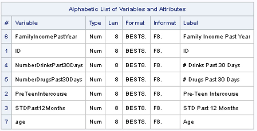
Output 3.1 shows the variables are all Type= Num (numeric) with n=15. For the sake of simplicity and ease of inspection, we use small data sets in this chapter but turn to larger data sets in later chapters. The description of each variable is as follows:
Family Income during the Past Year (FAMILYINCOMEPASTYEAR): continuous numeric variable representing family income during the past year
Case Identifier (ID): continuous numeric variable used as a case identifier
Number of Drinks Past 30 Days (NUMBERDRINKSPAST30DAYS): continuous numeric variable with a count of number of drinks during past 30 days
Number of Drugs Used Past 30 Days (NUMBERDRUGSPAST30DAYS): with a count of number of times used drugs during past 30 days
Sexual Intercourse Prior to Age 13 (PRETEENINTERCOURSE): numeric binary variable indicating if the respondent had sexual intercourse prior to age 13
Sexually Transmitted Disease Past 12 Months (STDPAST12MONTHS): numeric binary indicator indicating if the respondent had sexually transmitted disease during past 12 months
Age Interviewed (AGE): continuous numeric variable representing age at interview
As a prelude to the later sections of this book, we introduce a key method to examine the missing data pattern and group means: PROC MI with NIMPUTE=0 and a SIMPLE option. This approach to exploring missing data patterns and rates is used extensively because it provides a concise grid display of the missing data pattern, the amount of missing data for each variable and group as well as group means, and univariate and correlation statistics for the specified variables. This example uses a CLASS statement with the FCS statement to illustrate how to incorporate categorical variables such as indicators of having sexual intercourse prior to age 13 and having a sexually transmitted disease during the past 12 months.
proc mi data=teen_behavior nimpute=0 simple;
class preteenintercourse stdpast12months;
fcs;
var Id FamilyIncomePastYear NumberDrinksPast30Days NumberDrugsPast30Days
PreTeenIntercourse STDPast12Months age;
run;

Output 3.2 shows an arbitrary missing data pattern where PRETEENINTERCOURSE and FAMILYINCOMEPASTYEAR both have some missing data.

In Output 3.3, we see the result of specifying the SIMPLE option on the PROC MI statement. Note that the variables PRETEENINTERCOURSE and STDPAST12MONTHS are both coded as binary indicators with values of 0 or 1and are not treated as continuous variables in this exploratory analysis. The output includes standard univariate statistics as well as a count and percent of missing values for the continuous variables in the example data set. This option also produces estimates of pairwise correlations for the continuous variables.
For the imputation step, the binary indicator variables would be declared as classification variables in the CLASS statement, as demonstrated above. Our data exploration shows that two variables, PRETEENINTERCOURSE and FAMILYINCOMEPASTYEAR, have missing values that need to be imputed. The remaining fully observed variables (with the exception of the case ID) will be included in the multivariate imputation model.
3.3 Amount and Pattern of Missing Data
Evaluation of the amount and pattern of missing data is an important step in our multiple imputation. We briefly introduced this step in Section 3.2 but go into more detail here. This exploratory step will help to determine if the missing data problem can be addressed using PROC MI options for imputing monotone missing data (see Section 2.3.2) or requires one of the MCMC or FCS approaches that are appropriate for imputation of arbitrary patterns of missing data (see Section 2.3.3). Recall from Chapter 2 that in cases where the missing data pattern is arbitrary but the amount of missing data for all but a few variables is small, it is possible in SAS to use the MCMC method and MONOTONE option to convert the problem to a monotone pattern and then apply the MONOTONE procedure to complete the imputation for the remaining variables.
For now, let’s not worry about the exact multiple imputation method that we will use. We will cover that in detail in later chapters and examples. Let’s focus here on how to analyze the basic rates and pattern of missingness in our key variables. In practice, these missing data characteristics can be described and/or visualized through study of printouts from PROC PRINT (assuming the data set is small), frequency tables from PROC FREQ (best for classification variables), distribution analysis using PROC MEANS/PROC UNIVARIATE (best for continuous numeric variables), or through the use of PROC MI with the NIMPUTE=0 option.
As previously stated, the latter approach, using PROC MI and NIMPUTE=0 along with selected options, is a good choice for most situations as it provides a concise missing data pattern grid for all numeric variables in the data set. The grid displays the missing data pattern in a manner that allows easy evaluation of the pattern, that is, monotone, nearly monotone, or fully arbitrary. It also provides summary statistics such as variable means and frequency counts for the cases assigned to each unique grouping of cases (row of the grid) defined by patterns of observed and missing values. With use of the SIMPLE option we just introduced, you can also obtain overall univariate statistics such as the mean, standard deviation, minimum, and maximum of each variable.
For example, consider the data set, sample, created in the data step using the code below. The variable ID is used solely as a case identifier, HEARTBEAT represents number of heart beats per minute, and AGE contains age measured in years.
data sample;
input id heartbeat age;
datalines;
1 32 66
2 99 68
3 47 62
4 43 93
5 24 100
6 86 58
7 40 .
8 67 38
9 26 .
10 45 20
11 47 58
12 83 93
13 41 .
14 55 57
15 51 97
16 77 80
17 80 82
18 63 38
19 59 26
20 57 57
;
run;
Let’s examine the amount and pattern of missing data using both PROC PRINT and PROC MI (with the NIMPUTE=0 option).
proc print data=sample noobs;
run;

Output 3.4 shows that both variables, ID and HEARTBEAT, have fully observed data while AGE has missing data for 3 of the 20 records. Given the small size of the data set, it is easy to examine the missing data pattern visually and determine that this is a monotone missing data pattern with 15% missing data on AGE. Alternatively, we can use PROC MI with the NIMPUTE=0 option to conveniently obtain information on missing data amounts and patterns (without actually imputing any data at this point). Note that any classification variables would be treated as continuous since by default PROC MI assumes the MCMC method will be used when actual imputations are eventually created. (In this example, all variables are continuous.)
proc mi data=sample nimpute=0;
run;

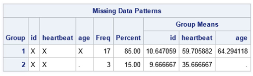
Output 3.5 reiterates that ID and HEARTBEAT have fully observed data with missing data for AGE on 3 of 20 records in this data set. The additional information in the “Model Information” output header simply lists the basic information about the various PROC MI settings including “Number of Imputations” set to zero (NIMPUTE=0). The other settings listed here will be discussed in more detail in later chapters.
The “Missing Data Patterns” grid shows two groups of data patterns: Group=1, which consists of those with fully observed data, indicated by an X, for each of the three variables; and Group=2, which indicates complete data on ID and HEARTBEAT but missing data, indicated by a ‘.’, for AGE. The remainder of the table provides summary statistics such as Frequency and Percent of cases for the data pattern and pattern-specific mean values for each variable. Note that the mean value for observed Group 1 values of HEARTBEAT is 59.71 beats/minute, while the mean for Group 2 is a much lower value of 35.67. This missing data pattern is considered univariate monotone.
3.4 Types of Variables to Be Imputed
Once the variables to be included in the imputation model and amount and pattern of missing data have been determined, the type and characteristics of the variable(s) to be imputed are addressed. Variable type in this context means either numeric or character. The variable type can be determined from PROC CONTENTS output. Furthermore, each variable that requires imputation can be characterized as continuous (numeric) or classification (either numeric or character). Note: the MI procedure allows use of either character or numeric classification variables, but continuous variables must be numeric. Determination of variable characteristics/type impacts the selection of an imputation method and model to be used in the imputation.
To illustrate, consider the data set, income. We use PROC PRINT to produce a list of this simple data set.
proc print noobs data=income;
run;
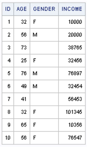
In Output 3.6, we see that the income data set includes four variables: ID=case identifier, AGE=age, GENDER=sex of respondent, and INCOME=respondent annual income. All but GENDER are numeric variables. ID serves as the unique case identifier, AGE and INCOME are fully observed and continuous, and GENDER is a binary, character variable with missing data for 2 of 10 records (represented by the default blank space). For a small data set with a limited number of records and variables, the printout approach is sufficient, but for larger data sets a more general set of tools is required.
Use of PROC CONTENTS to determine the SAS variable type followed by distribution analyses using PROC MEANS for numeric variables and PROC FREQ for classification variables typically serves us well for general data exploration. Let’s apply these techniques to the income data set.
proc contents data=income;
run;

Output 3.7 illustrates partial output from PROC CONTENTS, including the position, name, type, length, format, and informats for each variable in the data set. In the income data set, AGE, GENDER, and INCOME are Type=Numeric and GENDER is Type=Character.
For examination of variable distributions, PROC MEANS (for continuous variables) and PROC FREQ (for classification variables) are presented. Note that we include the options NMISS (PROC MEANS) and MISSING (on the PROC FREQ TABLES statement) to display the count of missing observations for each variable.
proc means data=income n nmiss mean min max;
run;

Output 3.8 provides details about each continuous variable, including the number of missing values (N Miss) as well as the Mean, Minimum, and Maximum of the nonmissing values. Here, we note no missing data on ID, AGE, or INCOME.
proc freq data=income;
tables gender / missing;
run;
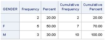
In Output 3.9, the frequency table for GENDER includes missing data represented by a blank space (the SAS default for character variables), “F” for female, and “M” for males. The two cases with missing data on GENDER represent 20% of the total sample. Outputs 3.6-3.9 provide key information such as variable type/characteristics, data values, amount of missing and observed data, and characteristics of variables available for imputation.
Use of PROC MI with a CLASS, VAR, and FCS statement along with NIMPUTE=0 will provide the missing data information/pattern for all variables in this data set, including the character classification variable GENDER.
proc mi data=income nimpute=0;
class gender;
fcs;
var id age income gender;
run;

Output 3.10 includes FCS model specification information, but given that no imputation is performed, these details are noted but left in the background. Had an imputation been executed, the FCS approach would have used the discriminant function method for imputing the missing values of the classification variable GENDER.
3.5 Imputation Methods
Thus far, we have considered the variables to be used in the imputation model, the amount and pattern of missing data, and the type of variables to be imputed. An important and related concern is what imputation method to use. Because the imputation methods available in SAS v9.4 were discussed in detail in Chapter 2, we will not repeat this information here. Practical guidance on choosing the method that is best suited to your imputation model will be provided for each application presented in later chapters.
3.6 Number of Imputations (MI Repetitions)
The number of MI repetitions needed is a common question. Early research showed that relative to the theoretical optimum where the number of independent MI repetitions is infinite (M=∞), high levels of relative efficiency (RE) could be achieved with as few as M=5 or M=10 replications. However, the statistic RE reported by SAS measures the proportion of information “recovered” (relative to the optimum) by the multiple imputation repetitions. It is a function of the size of the between (B) and within (W) imputation components of variance. As a brief reminder, in multiple imputation perfect efficiency of 1.0 can only be achieved with an infinite number of imputation repetitions, which is obviously not possible in practice. In general, as few as 5 to 10 imputations are needed for an acceptable relative efficiency (Rubin 1987). The RE formula is repeated here:
where λ is rate of missing information and M is the number of imputations.
For example, reconsider the missing data pattern grid from the sample data created in a previous data step.
proc mi data=sample nimpute=0;
run;
We observe that AGE has 15% missing data (3 of 20 records). Based on Table 61.7 from the PROC MI documentation, with M=5, relative efficiency of about .97 would be achieved and increasing the number of imputations will result in only modest incremental gains in relative efficiency. (Please refer to Table 61.7 in the PROC MI documentation for an overview of common M and rates of missing information.) Bear in mind that the rate of missing information is generally not equal to the missing data rate, as the missing information is a function of the within and between imputation variance for the imputation of AGE.
More recently, research into the relationship between the number of MI repetitions, M, and the achieved “coverage” of the 95% MI confidence intervals for parameter estimates has led to a recommendation to use larger numbers of MI repetitions to ensure that inferences remain unbiased for the target parameters. For example, Allison (http://www.statisticalhorizons.com/more-imputations) and Bodner (2008) suggest that a higher number of imputations will often result in more stable and accurate SEs, CIs, and p values. Given that the only penalty to requesting a higher number of replications in a SAS MI analysis (e.g., M=3 versus M=20) is increased computational processing, generating more imputation repetitions in return for more accuracy is a potentially beneficial approach. In this volume, most examples utilize examples based on a minimum of M=5 MI repetitions. As a matter of best practice in every data analysis, we recommend using a smaller number of MI repetitions (M=5 or M=10) in the exploratory phase of a data analysis with a repeat of the final analyses at a higher repetition count (e.g., M=30 to M=100). This “sensitivity analysis” will identify for the analyst whether key inferential statistics (e.g., CI half-widths, p-values for hypothesis tests) change in any statistically meaningful way. If significant change occurs when analyses are repeated at the higher repetition count, final results based on the more computationally intensive approach should be reported.
3.7 Overview of Multiple Imputation Procedures
PROC MI is designed to fill in missing data using one of several optional multiple imputation methods. This is step 1 in the three-step multiple imputation process. The MI statement is required and executes the procedure either using all defaults or with user-specified options to override default settings. As already demonstrated, this statement can be used to examine the missing data pattern through use of PROC MI with an optional NIMPUTE=0 specification for no imputations performed. After the initial examination of the missing data pattern and consideration of several issues that influence the imputation process, PROC MI is used to impute and create M imputed data sets.
The second step of the multiple imputation process is analysis of complete (imputed) data sets using standard SAS procedures or SAS SURVEY procedures. By default, PROC MI reports the multiple imputation estimates and inferential statistics for the unweighted mean of each continuous variable in the imputation model. However, MI estimates for many other univariate and multivariate statistics require the additional steps in which multiply imputed data generated by PROC MI are analyzed by SAS procedures and then combined for MI estimation and inference using PROC MIANALYZE. Typical examples of standard and corresponding SURVEY procedures are PROC MEANS (with a BY/DOMAIN group or similar technique since PROC MI provides means analyses by default)/PROC SURVEYMEANS for analysis of means, PROC FREQ/PROC SURVEYFREQ for analysis of frequency tables, PROC REG/PROC SURVEYREG/PROC GLM/PROC GENMOD, and so on for linear regression models, PROC PHREG/PROC SURVEYPHREG for survival analysis using Cox proportional hazards regression models, and PROC LOGISTIC/PROC SURVEYLOGISTIC for logistic regression with a variety of dependent variable types (binary, multinomial, ordinal) and link functions (e.g., logit, probit, complementary log-log options).
In step 2, SAS procedures are used to output a data set of statistics estimated for each MI repetition and organized for input into PROC MIANALYZE. For example, we use a BY _IMPUTATION_ statement to repeat the analysis for each of the multiple imputation repetitions in the input data set. The format of the output from the analysis of the m=1....M repetitions depends on the procedure used in the second step as well as the intended analysis from PROC MIANALYZE.
In the third and final step, PROC MIANALYZE combines results from step 2 to generate multiple imputation estimates and variances of estimates that permit the user to make statistical inferences from the MI data set. PROC MIANALYZE is considered a companion procedure to PROC MI in that it completes the three-step process.
These procedures and a variety of options will be demonstrated through many example applications presented in later chapters.
3.8 Multiple Imputation Example
This section presents an introductory multiple imputation example using the data set, housesprice3, which includes continuous and categorical variables and exhibits an arbitrary missing data pattern. In this example, we demonstrate the entire three-step multiple imputation process.
Our analysis goal is to perform a linear regression of house price (PRICE) on the square footage of the house (SQFEET) and number of bedrooms in the home (BEDRM).
We begin by using PROC CONTENTS and PROC MI without imputation to determine the type of variables that are to be included in the imputation model and the amount and pattern of missing data. We then proceed to multiply impute the missing data values, followed by regression analysis of the MI repetition data sets and use of PROC MIANALYZE to generate MI estimates and the corresponding inferential statistics for the regression model.
proc contents data=houseprice3;
run;

Output 3.12 consists of selected output from PROC CONTENTS and indicates that all variables are type=numeric with a length of 8.
We next use PROC MI without imputation (NIMPUTE=0) to examine the missing data pattern.
proc mi data=houseprice3 simple nimpute=0;
grun;

Output 3.13 reveals that the missing data pattern for the three variables is arbitrary, the two variables to be imputed (PRICE and SQFEET) are continuous, and the third variable, number of bedrooms (BEDRM), is fully observed. Before performing the actual imputation, it is useful to examine the marginal distribution of each variable to determine if the sample values are highly skewed or if there are extreme outlier values that could influence PROC MI’s estimation of the predictive distribution of the missing values.
Here, we use PROC SGPLOT to generate histograms with a superimposed normal curve and a boxplot for each of the two continuous variables, PRICE and SQFEET.
proc sgplot data=houseprice3;
histogram sqfeet; density sqfeet;
run;
proc sgplot data=houseprice3;
histogram price; density price;
run;


Figures 3.1 and 3.2 present histograms with superimposed normal curves. They provide an informal check of the normality assumption for the two continuous variables used in the imputation: SQFEET and PRICE. Although the small sample size for this example data set limits the ability to graphically analyze the properties of the data distributions, each variable appears to be relatively symmetrically, if not normally, distributed.
For the number of bedrooms in the home, BEDRM, we again use PROC SGPLOT to produce a horizontal bar graph.
proc sgplot data=houseprice3;
hbar bedrm;
run;
Figure 3.3: Horizontal Bar Chart of Number of Bedrooms in Home

The VBOX statement produces the vertical boxplots for SQFEET and PRICE.
proc sgplot data=houseprice3;
vbox sqfeet;
run;
proc sgplot data=houseprice3;
vbox price;
run;


Figures 3.4 and 3.5 present boxplots that provide a visual check of the distributions of the two continuous variables used in the imputation: SQFEET and PRICE. In these plots, we are looking for extreme outliers as well as the overall distribution of each variable. Neither Figures 3.1–3.2 nor Figures 3.4–3.5 provides strong evidence of a need for variable transformations in the imputation model. Because number of bedrooms is a categorical variable, it is not included in this evaluation.
Since the data exploration steps show that the variables to be imputed are both continuous with a fully observed categorical covariate and the data set has an arbitrary missing data pattern, the FCS imputation method is one appropriate choice. For this simple example, we use mainly default options but do specify a SEED value. The seed is used to initiate the generation of random numbers that are used in the imputation process. The specification of a fixed SEED value enables the analyst to exactly replicate the random number generation sequence and reproduce the results of a multiple imputation analysis run. For other settings, the defaults are used: M=5 repetitions and 20 burn-in iterations for the FCS method.
The imputation is executed using the code below.
proc mi data=houseprice3 out=out_imputed seed=678;
fcs regression (price sqfeet);
var sqfeet bedrm price;
run;
The VAR statement lists the variables to be used in the imputation, and the OUT= option specifies creation of the output data set out_imputed with individual data records identified by the automatic SAS variable called _IMPUTATION_ with values of 1–5 corresponding to the five repetitions of the imputation process.
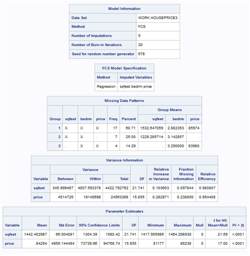
Output 3.14 displays the standard output from PROC MI for our imputation problem. The Variance Information included in this output pertains to the multiple imputation variance of the estimated means for the PRICE and SQFEET variables for which missing values have now been imputed.
The Parameter Estimates output also pertains to the estimates of the mean of PRICE and SQFEET and includes the combined MI standard error and MI 95% confidence limits for each mean. The MI degrees of freedom used to select the critical value of the Student t distribution for constructing the 95% CI for the mean of SQFEET is 21.741. As described in Section 2.5.3, PROC MI uses a special formula derived by Barnard and Rubin (1999) to estimate the degrees of freedom for the construction of the MI confidence interval for the true mean value of SQFEET and PRICE.
We next examine the output data set (by repetition) means for PRICE and SQFEET as an informal check of the imputation results. The five imputed data sets are contained in the out_imputed data set and are identified by the _IMPUTATION_ variable with values of 1–5. We expect the five means to be similar but not exactly the same given the variability of the MI process.
proc means data=out_imputed mean;
class _imputation_;
var price sqfeet;
run;
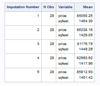
Each of the M=5 imputed data sets has a slightly different estimate of the mean value for SQFEET and PRICE due to the differing values imputed for the missing data (Output 3.15).
Although PROC MI has by default already provided MI estimates and CIs for the means of the SQFEET and PRICE variables, our assumed analytic objective in this exercise is to estimate the regression of PRICE on the square footage of the house and the number of bedrooms in the home. Therefore, we next use the PROC REG command with a BY statement to execute five separate regressions, one for each imputation repetition data set contained in the out_imputed data set.
The following PROC REG code shows how to create an output data set consisting of the regression model parameter estimates and their standard errors along with covariance information for subsequent use with PROC MIANALYZE. PROC REG produces an estimates (EST) data set that includes the regression parameter estimates and the corresponding estimated variance/covariance matrix for each of the five replications of the regression analysis. (Note: In this model we are treating the categorical variable BEDRM as continuous.) The printout of out_est in Output 3.16 highlights the structure and content of the output data set.
proc reg data=out_imputed outest=out_est covout;
model price=sqfeet bedrm ;
by _imputation_;
run;
proc print data=out_est noobs;
run;

From Output 3.16, first note that the _TYPE_=PARMS row includes the estimated regression parameters for each repetition’s covariates. Also note that the estimated parameters from the five regression models differ in value. For example, for repetition 1 (_IMPUTATION_=1), the parameter estimate for SQFEET=36.11, repetition 2=24.13, repetition 3=53.61, repetition 4=52.71, and repetition 5=33.01. The other estimates (BEDRM) show similar fluctuations across the M=5 repetitions. The additional rows contain the covariance matrix information for the regression parameter estimates (in this example a 3 x 3 matrix), identified by _TYPE_=COV for the five MI repetitions. The covariance information will ultimately be used in PROC MIANALYZE for estimation of the variances.
The third and final step in our analysis plan is to use PROC MIANALYZE to combine these five sets of regression estimates to produce final MI estimates of the regression model parameters, their standard errors, and 95% CIs for the true parameter values. For this step, the out_est data set from the PROC REG analysis of the MI repetition data sets (second step) is used as input to PROC MIANALYZE.
The following code illustrates use of PROC MIANALYZE to combine the MI repetition estimates to produce the final MI estimates, standard errors, and CIs for the regression model parameters. Use of the MODELEFFECTS statement, including the intercept followed by the model predictors, declares the effects used in the model. The EST (estimate) type of data set (here named out_est) includes both the needed parameter estimates (_TYPE_=PARMS) and the covariance matrices for the regression parameters (_TYPE_=COV) required by PROC MIANALYZE to complete the MI analysis for this linear regression model. In this example, we use an estimate type of output data set for use in PROC MIANALYZE, but many other types of data sets are also appropriate as input to PROC MIANALYZE. There are numerous examples of this process in action in Chapters 4 through 7 as well as in Chapter 8, which provides more detail on this particular issue.
proc mianalyze data=out_est;
modeleffects intercept sqfeet bedrm;
run;

Output 3.17 includes standard output from PROC MIANALYZE. Some of the key estimates included for each parameter are the between, within, and total variance; the relative increase in variance (due to the imputation); relative efficiency; and the fraction of missing information. Note that regression parameters for each predictor variable have a value for RE and fraction of missing information, even if there is no missing data on that particular variable. This is due to the fact that estimation of the regression coefficient includes the covariance of that variable with PRICE and SQFEET, which were subject to missing data.
The parameter estimates from the five regressions are averaged and the associated standard errors account for the imputation variability. The estimates would be interpreted in the usual manner for linear regression, keeping in mind that the estimates are averaged across the M imputed data sets. The estimated coefficient for SQFEET, a measure of a house’s square footage, implies that one additional square foot of house size results in an increase of about $39.91 in house price. And, one additional bedroom results in an increase of about $13,640 in the home price, always holding all other covariates constant. Both predictors are statistically significant at the alpha=.05 level.
3.9 Summary
This chapter has provided a checklist of preliminary data checks and the sequence of MI steps that are required when planning and executing a multiple imputation session in SAS. With this background and introductory example under our belts, we can now turn to more complex applications of the MI method for estimation and inference.